Chapter 9. Advanced Tools and Next Steps
This book has focused on the basics of football analytics using Python and R. We personally use both on a regular basis. However, we also use tools beyond these two programming languages. For people who want to keep growing, you will need to leave your comfort zone. This chapter provides an overview of other tools we use. We start with modeling tools that we use but have not mentioned yet, either because the topics are too advanced or because we could not find public data that would easily allow you to code along.
We then move on to computer tools. The topics are both disjointed and interwoven at the same time: you can learn one skill independently, but often, using one skill works best with other skills. As a football comparison, a linebacker needs to be able to defend the run, rush the passer, and cover players who are running pass routes, often in the same series of a game. Some skills (such as the ability to read a play) and player traits (such as speed) will help with all three linebacker situations, but they are often drilled separately. The most valuable players are great at all three.
This chapter is based on our experiences working as data scientists as well as an article Richard wrote for natural resource managers (“Paths to Computational Fluency for Natural Resource Educators, Researchers, and Managers”). We suggest you learn the topics in the order we present them, and we list reasons in Table 9-1. Once you gain some comfort with a skill, move on to another area. Eventually, you’ll make it back to a skill area and see where to grow in that area. As you learn more technologies, you can become better at learning new technologies!
Tip
In Build a Career in Data Science (Manning, 2020), Emily Robinson and Jacqueline Nolis provide broader coverage of skills for a career in data science.
| Tool | Reason | Examples |
|---|---|---|
Command line | Efficiently and automatically work with your operating system, use other tools that are command-line-only. | Microsoft PowerShell, bash, Zsh |
Version control | Keep track of changes to code, collaborate on code, share and publish code. | Git, Apache Subversion (SVN), Mercurial |
Linting | Clean code, provide internal consistency for style, reduce errors, and improve quality. | Pylint, lintr, Black |
Package creation and hosting | Reuse your own code, share your code internally or externally, and more easily maintain your code. | Conda, pip, CRAN |
Environment | Provide reproducible results, take models to production or the cloud, and ensure the same tools across collaborations. | Conda, Docker, Poetry |
Interactives and reports | Allow other people to explore data without knowing how to code, prototype tools before handing off to DevOps. | Jupyter Notebook, Shiny, Quarto |
Cloud | Deploy tools and advanced computing resources, share data. | Amazon Web Services (AWS), Microsoft Azure, Google Cloud Platform (GCP) |
Tip
All of the advanced tools we mention have free documentation either included with them or online. However, finding and using this documentation can be hard and often requires locating the proverbial diamonds in the rough. Hence, paid tutorials and resources such as books often, but not always, offer you a quality product. If you are a broke grad student, you might want to spend your time diving through the free resources to find the gems. If you are a working professional with kids and not much time, you probably want to pay for learning resources. Basically, finding quality learning materials comes down to time versus money.
Advanced Modeling Tools
Within this book, we have covered a wide range of models. For many people, these tools will be enough to advance your football analytics game. However, other people will want to go further and push the envelope. In this section, we describe some methods we use on a regular basis. Notice that many of these topics are interwoven. Hence, learning one topic might lead you to learn about another topic as well.
Time Series Analysis
Football data, especially feature-rich, high-resolution data within games, lends itself to look at trends through time. Time series analysis estimates trends through time. The methods are commonly used in finance, with applications in other fields such as ecology, physics, and social sciences. Basically, these models can provide better estimations when past observations are important for future predictions (also known as auto-correlations). Here are some resources we’ve found helpful:
-
Time Series Analysis and Its Application, 4th edition, by Robert H. Shumway and David S. Stoffer (Springer, 2017). Provides a detailed introduction to time series analysis using R.
-
Practical Time Series Analysis by Aileen Nielsen (O’Reilly, 2019) provides a gentler introduction to time series analysis with a focus on application, especially to machine learning.
-
Prophet by Facebook’s Core Data Science team is a time-series modeling tool that can be powerful when used correctly.
Multivariate Statistics Beyond PCA
Chapter 8 briefly introduced multivariate methods such as PCA and clustering. These two methods are the tip of the iceberg. Other methods exist, such as redundancy analysis (RDA), that allow both multivariate predictor and response variables. These methods form the basis of many entry-level unsupervised learning methods because the methods find their own predictive groups. Additionally, PCA assumes Euclidean distance (the same distance you may or may not remember from the Pythagorean theorem; for example, in two dimensions
Beyond direct application of these tools, understanding these methods will give you a firm foundation if you want to learn machine learning tools. Some books we learned from or think would be helpful include the following:
-
Numerical Ecology, 3rd edition, by Pierre Legendre and Louis Legendre (Elsevier, 2012) provides a generally accessible overview of many multivariate methods.
-
Analysis of Multivariate Time Series Using the MARSS Package vignette by E. Holmes, M. Scheuerell, and E. Ward comes with the MARSS package and may be found on the MARSS CRAN page. This detailed introduction describes how to do time series analysis with R on multivariate data.
Quantile Regression
Usually, regression models the average (or mean) expected value. Quantile regression models other parts of a distribution—specifically, a user-specified quantile. Whereas a boxplot (covered in “Boxplots”) has predefined quantiles, the user specifies which quantile they want with quantile regression. For example, when looking at NFL Scouting Combine data, you might wonder how player speeds change through time. A traditional multiple regression would look at the average player through time. A quantile regression would help you see if the faster players get faster through time. Quantile regression would also be helpful when looking at the NFL Draft data in Chapter 7. Resources for learning about quantile regression include the package documentation:
-
The
quantregpackage in R has a well-written 21-page vignette that is great regardless of language. -
The
statsmodelspackage in Python also has quantile regression documentation.
Bayesian Statistics and Hierarchical Models
Up to this point, our entire use of probability has been built on the assumption that events occur based on long-term occurrence, or frequency of events occurring. This type of probability is known as frequentist statistics. However, other views of probabilities exist.
Notably, a Bayesian perspective views the world in terms of degrees of belief or certainty. For example, a frequentist 95% confidence interval (CI) around a mean contains the mean 95% of the time, if you repeat your observations many, many, many times. Conversely, a Bayesian 95% credible interval (CrI) indicates a range for which you are 95% certain to contain the mean. It’s a subtle, but important, difference.
A Bayesian perspective begins with a prior understanding of the system, updates that understanding by using observed data, and then generates a posterior distribution. In practice, Bayesian methods offer three major advantages:
-
They can fit more complicated models when other methods might not have enough data.
-
They can include multiple sources of information more readily.
-
A Bayesian view of statistics is what many people have, even if they do not know the name for it.
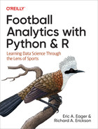
For example, consider picking which team will win. The prior information can either come from other data, your best guess, or any other source. If you are humble, you might think you will be right 50% of the time and would guess you would get two games right and two games wrong. If you are overconfident, you might think you will be right 80% of the time and get eight games right and two games wrong. If you are underconfident, you might think you will be right 20% of the time and get eight games wrong and two games right. This is your prior distribution.
For this example, a beta distribution gives you the probability distribution given the number of “successes” and “failures.” Graphically, this gives you Figure 9-1.

Figure 9-1. Prior distribution for predicting results of games
After observing 50 games, perhaps you were correct for 30 games and wrong for 20 games. A frequentist would say you are correct 60% of the time (30/50). To a Bayesian, this is the observed likelihood. With a Beta distribution, this would be 60 successes and 40 failures. Figure 9-2 shows the likelihood probability.
Next, a Bayesian multiplies Figure 9-1 by Figure 9-2 to create the posterior Figure 9-3. All three guesses are close, but the prior distribution informs the posterior.

Figure 9-2. Likelihood distribution for predicting results of games

Figure 9-3. In this posterior distribution for predicting results of games, notice the influence of the prior distribution on the posterior
This simple example illustrates how Bayesian methods work for an easy problem. However, Bayesian models also allow much more complicated models, such as multi-level models, to be fit (for example, to examine a regression with both team-level and player-level features). Additionally, Bayesian models’ posterior distribution captures uncertainty not also present with other estimation methods. For those of you wanting to know more about thinking like a Bayesian or doing Bayesian statistics, here are some books we have found to be helpful:
-
The Theory That Would Not Die: How Bayes’ Rule Cracked the Enigma Code, Hunted Down Russian Submarines, and Emerged Triumphant from Two Centuries of Controversy by Sharon Bertsch McGrayne (Yale University Press, 2011) describes how people have used Bayesian statistics to make decisions through high-profile examples such as the US Navy searching for missing nuclear weapons and submarines.
-
The Foundations of Statistics by Leonard J. Savage (Dover Press, 1972) provides an overview of how to think like a Bayesian, especially in the context of decision making such as betting or management.
-
Doing Bayesian Data Analysis, 2nd edition, by John Kruschke (Elsevier, 2014) is also known as the puppy book because of its cover. This book provides a gentle introduction to Bayesian statistics.
-
Bayesian Data Analysis, 3rd edition, by Andrew Gelman et al. (CRC Press, 2013). This book, often called BDA3 by Stan users, provides a rigorous and detailed coverage of Bayesian methods. Richard could not read this book until he had taken two years of advanced undergraduate and intro graduate-level math courses.
-
Statistical Rethinking: A Bayesian Course with Examples in R and Stan, 2nd edition, by Richard McElreath (CRC Press, 2020). This book is between the puppy book and BDA3 in rigor and is an intermediate-level text for people wanting to learn Bayesian statistics.
Survival Analysis/Time-to-Event
How long does a quarterback last in the pocket until he either throws the ball or is sacked? Time-to-event or survival analysis would help you answer that question. We did not cover this technique in the book because we could not find public data for this analysis. However, for people with more detailed time data, this analysis would help you understand how long until events occur. Some books we found useful on this topic include the following:
-
Regression Modeling Strategies: With Applications to Linear Models, Logistic and Ordinal Regression, and Survival Analysis, 2nd edition, by Frank E. Harrell Jr. (Springer, 2015). Besides being useful for regression, this book also includes survival analysis.
-
Think Stats, 2nd edition, by Allen B. Downey (O’Reilly, 2014) includes an accessible chapter on survival analysis using Python.
Bayesian Networks/Structural Equation Modeling
Chapter 8 alluded to the interconnectedness of data. Taking this a step further, sometimes data has no clear-cut cause or effect, or cause and effect variables are linked. For example, consider combine draft attributes. A player’s weight might be linked to a player’s running speed (for example, lighter players run quicker). Running speed and weight might both be associated with a running back’s rushing yards.
How to tease apart these confounding variables? Tools such as structural equation modeling and Bayesian networks allow these relations to be estimated. Here are some books we found to be helpful:
-
The Book of Why by Judea Pearl and Dana Mackenzie (Basic Books, 2018) walks through how to think about the world in terms of networks. The book also provides a great conceptual introduction to network models.
-
Bayesian Networks With Examples in R, 2nd edition, by Marco Scutari and Jean-Baptiste Denis (CRC Press, 2021) provides a nice introduction to Bayesian networks.
-
Structural Equation Modeling and Natural Systems by James B. Grace (Cambridge University Press, 2006) provides a gentle introduction to these models using ecological data.
Machine Learning
Machine learning is not any single tool but rather a collection of tools and a method of thinking about data. Most of our book has focused on statistical understanding of data. In contrast, machine learning thinks about how to use data to make predictions in an automated fashion.
Many great books exist on this topic, but we do not have any strong recommendations. Instead, build a solid foundation in math, stats, and programming, and then you should be well equipped to understand.
Command Line Tools
Command lines allow you to use code to interact with computers. Command lines have several related names, that, although having specific technical definitions, are often used interchangeably. One is shell, because this is the outside, or “shell,” of the operating system that humans, such as yourself, touch. Another is terminal because this is the software that uses the input and output text (historically, terminal referred to the hardware you used). As a more modern definition, this can refer to the software as well; for example, Richard’s Linux computer calls his command-line application the terminal. Lastly, console refers to the physical terminal. The Ask Ubuntu site provides detailed discussion on this topic, as well as some pictorial examples—notably, this answer.
Although these command-line tools are old (for example, Unix development started in the late 1960s), people still use them because of their power. For example, deleting thousands of files would likely take many clicks with a mouse but only one line of code at the command line.
When starting out, command lines can be confusing, just like starting with Python or R. Likewise, using the command line is a fundamental skill, similar to running or coordination drills in football. The command line is also used with most of the advanced skills we list and will also enhance your understanding of languages such as R or Python. For example, understanding the command line will enhance your understanding of programming languages by making you think about file structures and how computer operating systems work. But which command line to use?
We suggest you consider two options. First, the Bourne Again Shell (shortened to bash, named after the Bourne shell that it supersedes, which was named after the shell’s creator, Stephen Bourne) traditionally has been the default shell on Linux and macOS. This shell is also now available on Windows and is often the default for cloud computers (such as AWS, Microsoft Azure, and GCP) and high-performance supercomputers. Most likely, you will start with the bash shell.
A second option is Microsoft PowerShell. Historically, this was only for Windows, but is now available for other operating systems as well. PowerShell would be the best choice to learn if you also do a lot of information technology work in a corporate setting. The tools in PowerShell would be able to help you automate parts of your job such as security updates and software installs.
If you have macOS or Linux, you already have a terminal with a bash or bash-clone terminal (macOS switched to using the Zsh shell language because of copyright issues, but Zsh and bash are interchangeable for many situations, including our basic examples). Simply open the terminal app on your computer and follow along. If you use Windows, we suggest downloading Git for Windows, which comes with a lightweight bash shell. For Windows users who discover the utility of bash, you may eventually want to move to using Windows Subsystem for Linux (WSL). This program gives you a powerful, complete version of Linux on your Windows computer.
Bash Example
A terminal interface forces you to think about file structure on your computer. When you open your terminal, type pwd to print (on the screen) the current working directory. For example, on Richard’s Linux computer running Pop!_OS (a flavor of Linux), this looks like the following:
(base)raerickson@pop-os:~$pwd/home/raerickson
Here, /home/raerickson is the current working directory. To see the files in the working directory, type the list command, ls (we also think about ls as being short for list stuff as a way to remember the command):
raerickson@pop-os:~$lsDesktopGamesPublicDocumentsRUntitled.ipynbDownloadsminiconda3VideosFirefox_wallpaper.pngMusicTemplatesPicturestest.py
You can see all directories and files in Richard’s user directory. Filepaths are also important. The three basic paths to know are your current directory, your computer’s home directory, and up a level:
-
./is the current directory. -
~/is your computer’s default home directory. -
../is the previous directory.
For example, say your current directory is /home/raerickson. With this example, your directory structure would look like this:
-
../would be the home directory. -
./would be the raerickson directory. -
/would be the lowest level in your computer. -
~/would be the default home directory, which is /home/raerickson on Richard’s computer.
Note
For practical purposes, directory and folder are the same term and you can use either with the examples in this book.
You can use the change directory command, cd, to change your current working directory. For example, to get to the home directory, you could type this:
cd../
Or you could type this:
cd/home/
The first option uses a relative path. The second option uses an absolute path. In general, relative paths are better than absolute, especially for languages like Python and R, when other people might be reusing code across multiple machines.
You can also use the command line to move files and directories. For example, to copy test.py, you need to make sure you are in the same directory as the file. To do this, use cd to navigate to the directory with test.py. Type ls to make sure you can see the file. Then use cp (the copy function) to copy the file to Documents.
cptest.py./Documents
You can also use cp with different filepaths. For example, let’s say you’re in Documents and want to move test.py to python_code. You could use the filepaths with cp:
cp../test.py./python_code
In this example, you are currently in /home/raerickson/Documents. You can take the file from /home/raerickson/test.py/ by moving ../test.py to the directory /home/raerickson/Documents/python_code using ./python_code.
You can also copy directories. To do this, use the recursive option (or, in Linux parlance, flag) -r with the copy command. For example, to copy python_code, you would use cp ./python_code new_location. A move function also exists, which does not leave the original object behind. The move command is mv.
Warning
Command-line file deletions do not go to a recycling or trash directory on your computer. Deletions are permanent.
Lastly, you can remove directories and files by using the terminal. We recommend you be very careful. To delete, or remove, files, use rm file_name, where file_name is the file to delete. To delete a directory, use rm -r directory where directory is the directory you want to remove. To help you get started, Table 9-2 contains common bash commands we use on a regular basis.
| Command | Name and description |
|---|---|
| Print working directory, to show your location |
| Change directory, to change your location on your computer |
| Copy a file |
| Copy a directory |
| Move a file |
| Move a directory |
| Remove a file |
| Remove a directory |
Suggested Readings for bash
The bash shell is not only a way to interact with your computer, but it also comes with its own programming language. We generally only touch the surface of its tools in our daily work, but some people extensively program in the language. Here are some bash resources to learn more:
-
Software Carpentry offers free tutorials on the Unix Shell. More generally, we recommend this site as a general resource for many of the topics covered in this book.
-
Learning the bash Shell, 3rd edition, by Cameron Newham and Bill Rosenblatt (O’Reilly, 2005) provides introductions and coverage of the advanced tools and features of the language.
-
Data Science at the Command Line: Obtain, Scrub, Explore, and Model Data with Unix Power Tools, 2nd edition by Jeroen Janssens (O’Reilly, 2021) shows how to use helpful command-line tools.
-
We suggest your browse several books and find the one that meets your needs. Richard learned from Unix Shells by Example 4th edition, by Ellie Quigley (Pearson, 2004).
-
Online vendors offer courses on bash. We do not have any recommendations.
Version Control
When working on code on a regular basis, we face problems such as how do we keep track of changes? or how do we share code? The solution to this problem is version control software. Historically, several programs existed. These programs emerged from the need to collaborate and see what others did as well as to keep track of your own changes to code. Currently, Git is the major version control program; around the time of publication, it has a high market share, ranging from 70% to 90%.
Git emerged because Linus Torvalds faced that problem with the operating system he created, Linux. He needed a lightweight, efficient program to track changes from an army of volunteer programmers around the word. Existing programs used too much memory because they kept multiple versions of each file. Instead, he created a program that tracked only changes across files. He called this program Git.
Note
Fun fact: Linus Torvalds has, half-jokingly, claimed to name his two software programs after himself. Linux is a recursive acronym— Linux is not Unix (Linux)—but it is also close to his own first name. Git is British English slang for an arrogant person or jerk. Torvalds, by his own admission, can be difficult to work with. As an example, searching for images of Torvalds will show him responding to a reporter’s question with an obscene gesture.
Git
Git, at its heart, is an open source program that allows anybody to track changes to code. People can use Git on their own computer to track their own changes. We will start with some basic concepts of Git here. First, you need to obtain Git.
-
For Windows users, we like Git for Windows.
-
For macOS users, we encourage you to make sure you have Terminal installed. If you install Xcode, Git will be included, but this will be an older version. Instead, we encourage you to upgrade Git from the Git project home page.
-
For Linux users, we encourage you to upgrade the Git that comes with your OS to be safe.
-
For people wanting a GUI on Windows or macOS systems, we suggest you check out GitHub Desktop. The Git project page lists many other clients, including GUIs for Linux as well as Windows and macOS.
Tip
Command-line Git is more powerful than any GUI but is also more difficult. We show the concepts using the command line, but we encourage you to use a GUI. Two good options include GitHub’s GUI and the default Git GUI that comes with Git.
After obtaining Git, you need to tell Git where to keep track of your code:
-
Open a terminal.
-
Change your working directory to your project directory via
cd path/to_my_code/. -
In one line, type
git initthen press Enter/Return. Thegitcommand tells the terminal to use the Git program, andinittells the Git program to use theinitcommand. -
Tell Git what code to track. You can do this for individual files via
git add filenameor for all files withgit add .(The period is a shortcut for all files and directories in the current directory). -
Commit your changes to the code with
git commit -m "initial commit". With this command,gittells the terminal which program to use. Thecommitcommand tells git to commit. The flag-mtellscommitto accept the message in quotes,"my changes". With future edits, you will want to use descriptive terms here.
Warning
Be careful with which files you track. Seldomly will you want to track
data files (such as .csv files) or output files such as images or
tables. Be extra careful if posting code to public repositories such
as GitHub. You can use .gitignore files to block tracking for all file
types via commands such as *.csv to block tracking CSV files.
Now, you may edit your code. Let’s say you edit the file my_code.R and then change it. Type git status to see that this file has been changed. You may add the changes to the file by typing git add my_code.R. Then you need to commit the changes with git commit -m "example changes".
Tip
The learning curve for Git pays itself off if you accidentally delete one or more important files. Rather than losing days, weeks, months, or longer of work, you lose only the amount of time it takes you to search for undoing a delete with Git. Trust us; we know from experience and the school of hard knocks.
GitHub and GitLab
After you become comfortable with Git (at least comfortable enough to start sharing your code), you will want to back up and share code. When Richard was in grad school, around 2007, he had to use a terminal to remotely log on to his advisor’s computer and use Git to obtain code for his PhD project. He had to do this because easy-to-use commercial solutions (like GitHub) did not yet exist for sharing code. Luckily, commercial services now host Git repositories.
The largest provider is GitHub. This company and service are now owned by Microsoft. Its business model allows hosting for free but charges for business users and extra features for users. The second largest provider is GitLab. It has a similar business model but is also more developer focused. GitLab also includes an option for free self-hosting using its open source software. For example, O’Reilly Media and one of our employers both self-host their own GitLab repositories.
Regardless of which commercial platform you use, all use the same underlying Git technology and command-line tools. Even though the providers offer different websites, GUI tools, and bells and whistles, the underlying Git program is the same. Our default go-to is GitHub, but we know that some people prefer to avoid Microsoft and use GitLab. Another choice is Bitbucket, but we are less familiar with this platform.
The purpose of a remote repository is that your code is backed up there and other people can also access it. If you want, you can share your code with others. For open source software, people can report bugs as well as contribute new features and bug fixes for your software. We also like GitHub’s and GitLab’s online GUIs because they allow people to see who has updated and changed code. Another feature we like about these web pages is that they will render Jupyter Notebook and Markdown files as static web pages.
GitHub Web Pages and Résumés
A fun way to learn about Git and GitHub is to build a résumé. A search for GitHub résumés should help you find online tutorials (we do not include links because these pages are constantly changing). A Git-based résumé allows you to show your skills and create a marketable product demonstrating your skills. You can also use this to show off your football products, whether for fun or as part of job hunting. For example, we will have our interns create these pages as a way to document what they have learned while also learning Git better. Former intern John Oliver has an example résumé at https://oreil.ly/JOliv.
Suggested Reading for Git
Many resources can help you learn about Git, depending on your learning style. Some resources we have found to be useful include the following:
-
Git tutorials are offered on the Git project home page, including videos that provide an overview of the Git technology for people with no background.
-
Software Carpentry offers Git tutorials.
-
Training materials on GitHub provide resources. We do not provide a direct link because these change over time.
-
Git books from O’Reilly such as Version Control with Git, 3rd edition, by Prem Kumar Ponuthorai and Jon Loeliger (2022) can provide resources all in one location.
Style Guides and Linting
When we write, we use different styles. A text to our partner that we’re at the store might be At store, see u. followed by the response k. plz buy milk. A report to our boss would be very different, and a report to an external client even more formal. Coding can also have different styles. Style guides exist to create consistent code. However, programmers are a creative and pragmatic bunch and have created tools to help themselves follow styles. Broadly, these tools are called linting.
Note
The term linting comes from removing lint from clothes, like lint-rolling a sweater to remove specks of debris.
Different standards exist for different languages. For Python, PEP 8 is probably the most common style guide, although other style guides exist. For R, the Tidyverse/Google style guides are probably the most common style.
Note
Open source projects often split and then rejoin, ultimately becoming woven together. R style guides are no exception. Google first created an R Style Guide. Then the Tidyverse Style Guide based itself upon Google’s R Style Guide. But then, Google adapted the Tidyverse Style Guide for R with its own modifications. This interwoven history is described on the Tidyverse Style Guide page and Google’s R Style Guide page.
To learn more about the styles, please visit the PEP 8 Style Guide, Tidyverse style home pages, or Google’s style guides for many languages.
Note
Google’s style guides are hosted on GitHub using a Markdown language that is undoubtedly tracked using Git.
Table 9-1 lists some example linting programs. We also encourage you to look at the documentation for your code editor. These often will include add-ons (or plug-ins) that allow you to lint your code as you write.
Packages
We often end up writing custom functions while programming in Python or R. We need ways to easily reuse these functions and share them with others. We do this by placing the functions in packages. For example, Richard has created Bayesian models used for fisheries analysis that use the Stan language as called through R. He has released these models as an R package, fishStan. The outputs from these models are then used in a fisheries model, which has been released as a Python package.
With a package, we keep all our functions in the same place. Not only does this allow for reuse, but it also allows us to fix one bug and not hunt down multiple versions of the same file. We can also include tests to make sure our functions work as expected, even after updating or changing functions. Thus, packages allow us to create reusable and easy-to-maintain code.
We can use packages to share code with others. Probably the most common way to release packages is on GitHub repos. Because of the low barrier to entry, anyone can release packages. Python also has multiple package managers including pip and conda-forge, where people can submit packages. Likewise, R currently has one major package manager (and historically, had more): the Comprehensive R Archive Network (CRAN). These repositories have different levels of quality standards prior to submission, and thus some gatekeeping occurs compared to a direct release on sites like GitHub.
Suggested Readings for Packages
-
To learn about R packages, we used Hadley Wickham and Jennifer Bryan’s online book that is also available as a dead-tree version from O’Reilly.
-
To learn about Python packages, we used the Official Python tutorial, “Packaging Python Projects.”
Computer Environments
Imagine you run an R or Python package, but then the package does not run next session. Eventually, hours later, you figure out that a package was updated by its owner and now you need to update your code (yes, similar situations have occurred to us). One method to prevent this problem is to keep track of your computer’s environment. Likewise, computer users might have problems working with others. For example, Eric wrote this book on a Windows computer, whereas Richard used a Linux computer.
A computer’s environment is the computer’s collection of software and hardware. For example, you might be using a 2022 Dell XPS 13-inch laptop for your hardware. Your software environment might include your operating system (OS), such as Windows 11 release 22H2 (10.0.22621.1105), as well as the versions of R, Python, and their packages, such as R 4.1.3 with ggplot2 version 3.4.0. In general, most people are concerned about the programs for the computing environment. When an environment does not match across users (for example, Richard and Eric) or across time (for example, Eric’s computer in 2023 compared to 2021), programs will sometimes not run, such as the problem shown in Figure 9-4.
Tip
We cannot do justice for virtual environments like Conda in this book. However, many programmers and data scientists would argue their use helps differentiate experienced professionals from amateurs.
Tools like Conda let you lock down your computer’s environment and share the specific programs used. Tools like Docker go a step further and control not only the environment but also the operating systems. Both of these programs work best when the user understands the terminal.

Figure 9-4. Example of computer environments and how versions may vary across users and machines
Interactives and Report Tools to Share Data
Most people do not code. However, many people want access to data, and, hopefully, you want to share code. Tools for sharing data and models include interactive applications, or interactives. These allow people to interact with your code and results. For small projects, such as the ones some users may want to share after completing this book, programs like Posit’s Shiny or web-hosted Jupyter notebooks with widgets may meet your needs. People working in the data science industry, like Eric, will also use these tools to prototype models before handing the proof-of-concept tool over to a team of computer scientists to create a production-grade product.
Interactives work great for dynamic tools to see data. Other times, you may want or need to write reports. Markdown-based tools let you merge code, data, figures, and text all into one. For example, Eric writes reports to clients in R Markdown, Richard writes software documentation in Jupyter Notebook, Richard writes scientific papers in LaTeX, and this book was written in Quarto. If starting out, we suggest Quarto because the language expands upon R Markdown to also work with Python and other languages (R Markdown itself was created to be an easier-to-use version of LaTeX). Jupyter Notebook can also be helpful for reports and longer documents (for example, books have been written using Jupyter Notebook) but tend to work better for dynamic applications like interactives.
Artificial Intelligence Tools
Currently, tools exist that help people code using artificial intelligence (AI) or similar-type tools. For example, many code editors have autocompletion tools. These tools, at their core, are functionally AI. During the writing of this book, new AI tools have emerged that hold great potential to assist people coding. For example, ChatGPT can be used to generate code based on user input prompts. Likewise, programs such as GitHub Copilot help people code based on input prompts, and Google launched its own competing program, Codey.
However, AI tools are still new, and challenges exist with their use. For example, the tools will produce factual errors and well-documented biases. Besides well documented factual errors and biases, the programs consume user data. Although this helps create a better program through feedback, people can accidentally release data they did not intend to release. For example, Samsung staff accidentally released semiconductor software and proprietary data to ChatGPT. Likewise, the Copilot for Business Privacy Statement notes that “it collects data to provide the service, some of which is then saved for further analysis and product improvements.”
Warning
Do not upload data and code to AI services unless you understand how the services may use and store your data and code.
We predict that AI-based coding tools will greatly enhance coding but also require skilled operators. For example, spellcheckers and grammar checkers did not remove the need for editors. They simply reduced one part of editors’ jobs.
Conclusion
American football is the most popular sport in the US and one of the most popular sports in the world. Millions of fans travel countless miles to see their favorite teams every year, and more than a billion dollars in television deals are signed every time a contract is ready to be renewed. Football is a great vehicle for all sorts of involvement, whether that be entertainment, leisure, pride, or investment. Now, hopefully, it is also a vehicle for math.
Throughout this book, we’ve laid out the various ways in which a mathematically inclined person could better understand the game through statistical and computational tools learned in many undergraduate programs throughout the world. These very same approaches have helped us as an industry push the conversation forward into new terrain, where analytically driven approaches are creating new problems for us to solve, which will no doubt create additional problems for you, the reader of this book, to solve in the future.
The last decade of football analytics has seen us move the conversation toward the “signal and the noise” framework popularized by Nate Silver. For example, Eric and his former coworker George Chahrouri asked the question “if we want to predict the future, should we put more stock in how a quarterback plays under pressure or from a clean pocket?” in a PFF article.
We’ve also seen a dramatic shift in the value of players by position, which has largely been in line with the work of analytical firms like PFF, which help people construct rosters by valuing positions. Likewise, websites like https://rbsdm.com have allowed fans, analysts, and scribes to contextualize the game they love and/or cover using data.
On a similar note, the legalization of sports betting across much of the US has increased the need to be able to tease out the meaningful from the misleading. Even the NFL Draft, at one point an afterthought in the football calendar, has become a high-stakes poker game and, as such, has attracted the best minds in the game working on making player selection, and asset allocation, as efficient as possible.
The future is bright for football analytics as well. With the recent proliferation of player-tracking data, the insights from this book should serve as a jumping-off point in a field with an ever-growing set of problems that should make the game more enjoyable. After all, almost every analytical advancement in the game (more passing, more fourth-down attempts) has made the game more entertaining. We predict that trend will continue.
Furthermore, sports analytics in general, and football analytics specifically, has opened doors for many more people to participate in sports and be actively engaged than in previous generations. For example, Eric’s internship program, as of May of 2023, has sent four people into NFL front offices, with hopefully many more to come. By expanding who can participate, as well as add value to the game, football now has the opportunity to become a lot more compelling for future generations.
Hopefully, our book has increased your interest in football and football analytics. For someone who just wants to dabble in this up-and-coming field, perhaps it contains everything you need. For those who want to gain an edge in fantasy football or in your office pool, you can update our examples to get the current year’s data. For people seeking to dive deeper, the references in each chapter should provide a jumping-off point for future inquiry.
Lastly, here are some websites to look at for more football information:
-
Eric’s current employer, SumerSports: https://sumersports.com/
-
Eric’s former employer, PFF: https://www.pff.com
-
A website focusing on advanced NFL stats, Football Outsiders: https://www.footballoutsiders.com
-
Ben Baldwin’s page that links to many other great resources: https://rbsdm.com
Happy coding as you dive deeper into football data!