
Chapter 8
Using Recursive Functions
IN THIS CHAPTER
![]() Defining recursion and how it works
Defining recursion and how it works
![]() Using recursion to perform advanced tasks
Using recursion to perform advanced tasks
![]() Mixing recursion with functions
Mixing recursion with functions
![]() Understanding common recursion errors
Understanding common recursion errors
Some people confuse recursion with a kind of looping. The two are completely different sorts of programming and wouldn’t even look the same if you could view them at a low level. In recursion, a function calls itself repetitively and keeps track of each call through stack entries, rather than an application state, until the condition used to determine the need to make the function call meets some requirement. At this point, the list of stack entries unwinds with the function passing the results of its part of the calculation to the caller until the stack is empty and the initiating function has the required output of the call. Although this sounds mind-numbingly complex, in practice, recursion is an extremely elegant method of solving certain computing problems and may be the only solution in some situations. This chapter introduces you to the basics of recursion using the two target languages for this book, so don’t worry if this initial definition leaves you in doubt of what recursion means.
Of course, you might wonder just how well recursion works on some common tasks, such as iterating a list, dictionary, or set. This chapter discusses all the basic requirements for replacing loops with recursion when interacting with common data structures. It then moves on to more advanced tasks and demonstrates how using recursion can actually prove superior to the loops you used in the past — not to mention that it can be easier to read and more flexible as well. Of course, when using other programming paradigms, you’ll likely continue using loops because those languages are designed to work with them.
 One of the most interesting aspects of using first-class functions in the functional programming paradigm is that you can now pass functions rather than variables to enable recursion. This capability makes recursion in the functional programming paradigm significantly more powerful than it is in other paradigms because the function can do more than a variable, and by passing different functions, you can alter how the main recursion sequence works.
People understand loops with considerably greater ease because we naturally use loops in our daily lives. Every day, you perform repetitive tasks a set number of times or until you satisfy a certain condition. You go to the store, know that you need a dozen nice apples, and count them out one at a time as you place them in one of those plastic bags. The lack of recursion in our daily lives is one of the reasons that it’s so hard to wrap our brains around recursion, and it's why people make so many common mistakes when using recursion. The end of the chapter discusses a few common programming errors so that you can successfully use recursion to create an amazing application.
Performing Tasks More than Once
One of the main advantages of using a computer is its capability to perform tasks repetitively — often far faster and with greater accuracy than a human can. Even a language that relies on the functional programming paradigms requires some method of performing tasks more than once; otherwise, creating the language wouldn't make sense. Because the conditions under which functional languages repeat tasks differ from those of other languages using other paradigms, thinking about the whole concept of repetition again is worthwhile, even if you’ve worked with these other languages. The following sections provide you with a brief overview.
Defining the need for repetition
The act of repeating an action seems simple enough to understand. However, repetition in applications occurs more often than you might think. Here are just a few uses of repetition to consider:
- Performing a task a set number of times
- Performing a task a variable number of times until a condition is met
- Performing a task a variable number of times until an event occurs
- Polling for input
- Creating a message pump
- Breaking a large task into smaller pieces and then executing the pieces
- Obtaining data in chunks from a source other than the application
- Automating data processing using various data structures as input
In fact, you could easily create an incredibly long list of repeated code elements in most applications. The point of repetition is to keep from writing the same code more than once. Any application that contains repeated code becomes a maintenance nightmare. Each routine must appear only once to make its maintenance easy, which means using repetition to allow execution more than one time.
 Without actual loop statements, the need for repetition becomes significantly clearer because repetition suddenly receives the limelight. Thinking through the process of repeating certain acts without relying on state or mutable variables takes on new significance. In fact, the difficulty of actually accomplishing this task in a straightforward manner forces most language designers to augment even pure languages with some sort of generalized looping mechanism. For example, Haskell provides the
 forM function, which actually has to do with performing I/O (see the article at http://learnyouahaskell.com/input-and-output for details). The Control.Monad library contains a number of interesting loop-like functions that really aren't loops; they’re functions that implement repetition using data structures as input (see https://hackage.haskell.org/package/base-4.2.0.1/docs/Control-Monad.html for details). Here's an example of forM in use:
import Control.Monad
values <- forM [1, 2, 3, 4]
   (a -> do
      putStrLn $ "The value is: " ++ show a )
In this case, forM processes a list containing four values, passing it to the lambda function that follows. The lambda function simply outputs the values using putStrLn and show a. Figure 8-1 shows the output from this example. Obviously, impure languages, such as Python, do provide the more traditional methods of repeating actions.

FIGURE 8-1: Even Haskell provides a looping-type mechanism in the form of functions.
Using recursion instead of looping
The functional programming paradigm doesn't allow the use of loops for two simple reasons. First, a loop requires the maintenance of state, and the functional programming paradigm doesn’t allow state. Second, loops generally require mutable variables so that the variable can receive the latest data updates as the loop continues to perform its task. As mentioned previously, you can’t use mutable variables in functional programming. These two reasons would seem to sum up the entirety of why to avoid loops, but there is yet another.
One of the reasons that functional programming is so amazing is that you can use it on multiple processors without concern for the usual issues found with other programming paradigms. Because each function call is guaranteed to produce precisely the same result, every time, given the same inputs, you can execute a function on any processor without regard to the processor use for the previous call. This feature also affects recursion because recursion lacks state.
When a function calls itself, it doesn’t matter where the next function call occurs; it can occur on any processor in any location. The lack of state and mutable variables makes recursion the perfect tool for using as many processors as a system has to speed applications as much as possible.
Understanding Recursion
Recursion, in its essence, is a method of performing tasks repetitively, wherein the original function calls itself. Various methods are available for accomplishing this task, as described in the following sections. The important aspect to keep in mind, though, is the repetition. Whether you use a list, dictionary, set, or collection as the mechanism to input data is less important than the concept of a function's calling itself until an event occurs or it fulfills a specific requirement.
Considering basic recursion
This section discusses basic recursion, which is the kind that you normally see demonstrated for most languages. In this case, the doRep function creates a list containing a specific number, n, of a value, x, as shown here for Python:
def doRep(x, n):
   y = []
   if n == 0:
      return []
   else:
      y = doRep(x, n - 1)
      y.append(x)
      return y
To understand this code, you must think about the process in reverse. Before it does anything else, the code actually calls doRep repeatedly until n == 0. So, when n == 0, the first actual step in the recursion process is to create an empty list, which is what the code does.
At this point, the call returns and the first actual step concludes, even though you have called doRep six times before it gets to this point. The next actual step, when n == 1, is to make y equal to the first actual step, an empty list, and then append x to the empty list by calling y.append(x). At this point, the second actual step concludes by returning [4] to the previous step, which has been waiting in limbo all this time.
The recursion continues to unwind until n == 5, at which point it performs the final append and returns [4, 4, 4, 4, 4] to the caller, as shown in Figure 8-2.
![Screen capture of python window with code ending return y, doRep(4, 5) with the output [4, 4, 4, 4, 4].](http://imgdetail.ebookreading.net/202009/02/9781119527503/9781119527503__functional-programming-for__9781119527503__images__9781119527503-fg0802.png)
FIGURE 8-2: Recursion almost seems to work backward when it comes to code execution.
Sometimes it's incredibly hard to wrap your head around what happens with recursion, so putting a print statement in the right place can help. Here’s a modified version of the Python code with the print statement inserted. Note that the print statement goes after the recursive call so that you can see the result of making it. Figure 8-3 shows the flow of calls in this case.
def doRep(x, n):
   y = []
   if n == 0:
      return []
   else:
      y = doRep(x, n - 1)
      print(y)
      y.append(x)
      return y
![Screen capture of python window with code ending y.append(x); return y, doRep(4, 5) with the output one below the other: [], [4], [4, 4], [4, 4, 4], [4, 4, 4, 4], [4, 4, 4, 4, 4].](http://imgdetail.ebookreading.net/202009/02/9781119527503/9781119527503__functional-programming-for__9781119527503__images__9781119527503-fg0803.png)
FIGURE 8-3: Adding a print statement in the right place can make recursion easier to understand.
Performing the same task in Haskell requires about the same code, but with a Haskell twist. Here's the same function written in Haskell:
doRep x n | n <= 0 = [] | otherwise = x:doRep x (n-1)
The technique is the same as the Python example. The function accepts two inputs, x (the number to append) and n (the number of times to append it). When n is 0, the Haskell code returns an empty list. Otherwise, Haskell appends x to the list and returns the appended list. Figure 8-4 shows the functionality of the Haskell example.
![Screen capture of WinGHCi window with code doRep x n | n <= 0 = [] | otherwise = x:doRep x (n-1); doRep 4 5 with the output [4, 4, 4, 4, 4].](http://imgdetail.ebookreading.net/202009/02/9781119527503/9781119527503__functional-programming-for__9781119527503__images__9781119527503-fg0804.png)
FIGURE 8-4: Haskell also makes creating the doRep function easy.
Performing tasks using lists
Lists represent multiple inputs to the same call during the same execution. A list can contain any data type in any order. You use a list when a function requires more than one value to calculate an output. For example, consider the following Python list:
myList = [1, 2, 3, 4, 5]
If you wanted to use standard recursion to sum the values in the list and provide an output, you could use the following code:
def lSum(list):
   if not list:
      return 0
   else:
      return list[0] + lSum(list[1:])
The function relies on slicing to remove one value at a time from the list and add it to the sum. The base case (principle, simplest, or foundation) is that all the values are gone and now list contains the empty set, ([]), which means that it has a value of 0. To test this example out, you type lSum(myList) and press Enter.
Using lambda functions in Python recursion isn't always easy, but this particular example lends itself to using a lambda function quite easily. The advantage is that you can create the entire function in a single line, as shown in the following code (with two lines, but using a line-continuation character):
lSum2 = lambda list: 0 if not list
   else list[0] + lSum2(list[1:])
The code works precisely the same as the longer example, relying on slicing to get the job done. You use it in the same way, typing lSum2(myList) and pressing Enter. The result is the same, as shown in Figure 8-5.
![Screen capture of python window with code ending return list[0] + lSum(list[1:]); lSum<list> with output 15; and code ending else list[0] + lSum2(list[1:]) lSum2<list> with output 15.](http://imgdetail.ebookreading.net/202009/02/9781119527503/9781119527503__functional-programming-for__9781119527503__images__9781119527503-fg0805.png)
FIGURE 8-5: Use lists for multiple simple entries to the same function call.
Upgrading to set and dictionary
Both Haskell and Python support sets, but with Python, you get them as part of the initial environment, and with Haskell, you must load the Data.Set library (see http://hackage.haskell.org/package/containers-0.5.11.0/docs/Data-Set.html to obtain the required support). Sets differ from lists in that sets can't contain any duplicates and are generally presented as ordered. In Python, the sets are stored as hashes. In some respects, sets represent a formalization of lists. You can convert lists to sets in either language. Here’s the Haskell version:
import Data.Set as Set
myList = [1, 4, 8, 2, 3, 3, 5, 1, 6]
mySet = Set.fromList(myList)
mySet
which has an output of fromList [1,2,3,4,5,6,8] in this case. Note that even though the input list is unordered, mySet is ordered when displayed. Python relies on the set function to perform the conversion, as shown here:
myList = [1, 4, 8, 2, 3, 3, 5, 1, 6]
mySet = set(myList)
mySet
The output in this case is {1, 2, 3, 4, 5, 6, 8}. Notice that sets in Python use a different enclosing character, the curly brace. The unique and ordered nature of sets makes them easier to use in certain kinds of recursive routines, such as finding a unique value.
 You can find a number of discussions about Haskell sets online, and some people are even unsure as to whether the language implements them as shown at
 https://stackoverflow.com/questions/7556573/why-is-there-no-built-in-set-data-type-in-haskell. Many Haskell practitioners prefer to use lists for everything and then rely on an approach called list comprehensions to achieve an effect similar to using sets, as described at http://learnyouahaskell.com/starting-out#im-a-list-comprehension. The point is that if you want to use sets in Haskell, they are available.
A dictionary takes the exclusivity of sets one step further by creating key/value pairs, in which the key is unique but the value need not be. Using keys makes searches faster because the keys are usually short and you need only to look at the keys to find a particular value. Both Haskell and Python place the key first, followed by the value. However, the methods used to create a dictionary differ. Here's the Haskell version:
let myDic = [("a", 1), ("b", 2), ("c", 3), ("d", 4)]
Note that Haskell actually uses a list of tuples. In addition, many Haskell practitioners call this an association list, rather than a dictionary, even though the concept is the same no matter what you call it. Here’s the Python form:
myDic = {"a": 1, "b": 2, "c": 3, "d": 4}
Python uses a special form of set to accomplish the same task. In both Python and Haskell, you can access the individual values by using the key. In Haskell, you might use the lookup function: lookup "b" myDic, to find that b is associated with 2. Python uses a form of index to access individual values, such as myDic["b"], which also accesses the value 2.
You can use recursion with both sets and dictionaries in the same manner as you do lists. However, recursion really begins to shine when it comes to complex data structures. Consider this Python nested dictionary:
myDic = {"A":{"A": 1, "B":{"B": 2, "C":{"C": 3}}}, "D": 4}
In this case, you have a dictionary nested within other dictionaries down to four levels, creating a complex dataset. In addition, the nested dictionary contains the same "A" key value as the first level dictionary (which is allowed), the same "B" key value as the second level, and the "C" key on the third level. You might need to look for the repetitious keys, and recursion is a great way to do that, as shown here:
def findKey(obj, key):
   for k, v in obj.items():
      if isinstance(v, dict):
         findKey(v, key)
      else:
         if key in obj:
            print(obj[key])
This code looks at all the entries by using a for loop. Notice that the loop unpacks the entries into key, k, and value, v. When the value is another dictionary, the code recursively calls findKey with the value and the key as input. Otherwise, if the instance isn't a dictionary, the code checks to verify that the key appears in the input object and prints just the value of that object. In this case, an object can be a single entry or a sub-dictionary. Figure 8-6 shows this example in use.
![Screen capture of python window with code ending print(obj[key]); findKey(MyDic, “A”); findKey(MyDic, “B”); findKey(MyDic, “C”); findKey(MyDic, “D”) with output ending 1; 2; 3; 4.](http://imgdetail.ebookreading.net/202009/02/9781119527503/9781119527503__functional-programming-for__9781119527503__images__9781119527503-fg0806.png)
FIGURE 8-6: Dictionaries can provide complex datasets you can parse recursively.
Considering the use of collections
Depending on which language you choose, you might have access to other kinds of collections. Most languages support lists, sets, and dictionaries as a minimum, but you can see some alternatives for Haskell at http://hackage.haskell.org/package/collections-api-1.0.0.0/docs/Data-Collections.html and Python at https://docs.python.org/3/library/collections.html. All these collections have one thing in common: You can use recursion to process their content. Often, the issue isn’t one of making recursion work, but of simply finding the right technique for accessing the individual data elements.
Using Recursion on Lists
The previous sections of the chapter prepare you to work with various kinds of data structures by using recursion. You commonly see lists used whenever possible because they’re simple and can hold any sort of data. Unfortunately, lists can also be quite hard to work with because they can hold any sort of data (most analysis requires working with a single kind of data) and the data can contain duplicates. In addition, you might find that the user doesn’t provide the right data at all. The following sections look at a simple case of looking for the next and previous values in the following list of numbers:
myList = [1,2,3,4,5,6]
Working with Haskell
This example introduces a few new concepts from previous examples because it seeks to provide more complete coverage. The following code shows how to find the next and previous values in a list:
findNext :: Int -> [Int] -> Int
findNext _ [] = -1
findNext _[_] = -1
findNext n (x:y:xs)
    | n == x = y
    | otherwise = findNext n (y:xs)

findPrev :: Int -> [Int] -> Int
findPrev _ [] = -1
findPrev _[_] = -1
findPrev n (x:y:xs)
    | n == y = x
    | otherwise = findPrev n (y:xs)
In both cases, the code begins with a type signature that defines what is expected regarding inputs and outputs. As you can see, both functions require Int values for input and provide Int values as output. The next two lines provide outputs that handle the cases of empty input (a list with no entries) and singleton input (a list with one entry). There is no next or previous value in either case.
The meat of the two functions begins by breaking the list into parts: the current entry, the next entry, and the rest of the list. So, the processing begins with x = 1, y = 2, and xs = [3,4,5,6]. The code begins by asking whether n equals x for findNext and whether n equals y for findPrev. When the two are equal, the function returns either the next or previous value, as appropriate. Otherwise, it recursively calls findNext or findPrev with the remainder of the list. Because the list gets one item shorter with each recursion, processing stops with a successful return of the next or previous value, or with -1 if the list is empty. Figure 8-7 shows this example in use. The figure presents both successful and unsuccessful searches.
![Screen capture of WinGHCi window with find.hs loaded and *Main> code myList = [1, 2, 3, 4, 5, 6] with codes, outputs: findNext 4 myList, 5; findNext 4 myList, 3; findNext 0 myList, -1; findNext 4 [] myList, -1.](http://imgdetail.ebookreading.net/202009/02/9781119527503/9781119527503__functional-programming-for__9781119527503__images__9781119527503-fg0807.png)
FIGURE 8-7: The findNext and findPrev functions help you locate items in a list.
Working with Python
The Python version of the code relies on lambda functions because the process is straightforward enough to avoid using multiple lines. Here is the Python code used for this example:
findNext = lambda x, obj: -1 if len(obj) == 0
   or len(obj) == 1
   else obj[1] if x == obj[0]
      else findNext(x, obj[1:])

findPrev = lambda x, obj: -1 if len(obj) == 0
   or len(obj) == 1
   else obj[0] if x == obj[1]
      else findPrev(x, obj[1:])
Normally, you could place everything on a single line; this example uses line-continuation characters to accommodate this book's margins. As with the Haskell code, the example begins by verifying that the incoming list contains two or more values. It also returns -1 when there is no next or previous value to find. The essential mechanism used, a comparison, is the same as the Haskell example. In this case, the Python code relies on slicing to reduce the size of the list on each pass. Figure 8-8 shows this example in action using both successful and unsuccessful searches.
![Screen capture of python window with code ending else findPrev(x, obj[1:]) and codes, outputs: findNext 4 myList, 5; findNext 4 myList, 3; findNext 0 myList, -1; findNext 4 [] myList, -1.](http://imgdetail.ebookreading.net/202009/02/9781119527503/9781119527503__functional-programming-for__9781119527503__images__9781119527503-fg0808.png)
FIGURE 8-8: Python uses the same mechanism as Haskell to find matches.
Passing Functions Instead of Variables
This section looks at passing functions to other functions, using a technique that is one of the most powerful features of the functional programming paradigm. Even though this section isn’t strictly about recursion, you can use the technique in it with recursion. The example code is simplified to make the principle clear.
Understanding when you need a function
Being able to pass a function to another function provides much needed flexibility. The passed function can modify the receiving function’s response without modifying that receiving function’s execution. The two functions work in tandem to create output that’s an amalgamation of both.
Normally, when you use this function-within-a-function technique, one function determines the process used to produce an output, while the second function determines how the output is achieved. This isn’t always the case, but when creating a function that receives another function as input, you need to have a particular goal in mind that actually requires that function as input. Given the complexity of debugging this sort of code, you need to achieve a specific level of flexibility by using a function rather than some other input.
Also tempting is to pass a function to another function to mask how a process works, but this approach can become a trap. Try to execute the function externally when possible and input the result instead. Otherwise, you might find yourself trying to discover the precise location of a problem, rather than processing data.
Passing functions in Haskell
Haskell provides some interesting functionality, and this example shines a light on some of it. The following code shows the use of Haskell signatures to good effect when creating functions that accept functions as input:
doAdd :: Int -> Int -> Int
doAdd x y = x + y

doSub :: Int -> Int -> Int
doSub x y = x - y

cmp100 :: (Int -> Int -> Int) -> Int -> Int -> Ordering
cmp100 f x y = compare 100 (f x y)
The signatures and code for both doAdd and doSub are straightforward. Both functions receive two integers as input and provide an integer as output. The first function simply adds to values; the second subtracts them. The signatures are important to the next step.
The second step is to create the cmp100 function, which accepts a function as the first input. Notice the (Int -> Int -> Int) part of the signature. This section indicates a function (because of the parentheses) that accepts two integers as input and provides an integer as output. The function in question can be any function that has these characteristics. The next part of the signature shows that the function will receive two integers as input (to pass along to the called function) and provide an order as output.
The actual code shows that the function is called with the two integers as input. Next, compare is called with 100 as the first value and the result of whatever happens in the called function as the second input. Figure 8-9 shows the example code in action. Notice that the two numeric input values provide different results, depending on which function you provide.
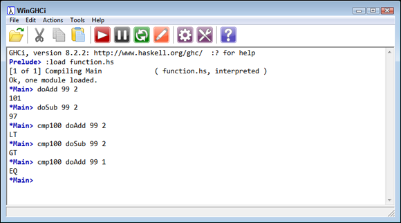
FIGURE 8-9: Depending on the function you pass, the same numbers produce different results.
Passing functions in Python
For the example in this section, you can't use a lambda function to perform the required tasks with Python, so the following code relies on standard functions instead. Notice that the functions are the same as those provided in the previous example for Haskell and they work nearly the same way.
def doAdd(x, y):
   return x + y

def doSub(x, y):
   return x - y

def compareWithHundred(function, x, y):
   z = function(x, y)
   out = lambda x: "GT" if 100 > x
      else "EQ" if 100 == x else "LT"
   return out(z)
The one big difference is that Python doesn’t provide a compare function that provides the same sort of output as the Haskell compare function. In this case, a lambda function performs the comparison and provides the proper output. Figure 8-10 shows this example in action.

FIGURE 8-10: Python makes performing the comparison a bit harder.
Defining Common Recursion Errors
Recursion can actually cause quite a few problems — not because recursion is brittle or poorly designed, but because developers don't rely on it very often. In fact, most developers avoid using recursion because they see it as hard when it truly isn’t. A properly designed recursive routine has an elegance and efficiency not found in other programming structures. With all this said, developers still do make some common errors when using recursion, and the following sections give you some examples.
Forgetting an ending
When working with looping structures, you can see the beginning and end of the loop with relative ease. Even so, most looping structures aren’t foolproof when it comes to providing an exit strategy, and developers do make mistakes. Recursive routines are harder because you can’t see the ending. All you really see is a function that calls itself, and you know where the beginning is because it’s where the function is called initially.
Recursion doesn’t rely on state, so you can’t rely on it to perform a task a set number of times (as in a for loop) and then end unless you design the recursion to end in this manner. Likewise, even though recursion does seem like a while statement because it often relies on a condition to end, it doesn’t use a variable, so there is nothing to update. Recursion does end when it detects an event or meets a condition, but the circumstances for doing so differ from loops. Consequently, you need to exercise caution when using recursion to ensure that the recursion will end before the host system runs out of stack space to support the recursive routine.
Passing data incorrectly
Each level of recursion generally requires some type of data input. Otherwise, knowing whether an event has occurred or a condition is met becomes impossible. The problem isn’t with understanding the need to pass data, it’s with understanding the need to pass the correct data. When most developers write applications, the focus is on the current level — that is, where the application is at now. However, when working through a recursion problem, the focus is instead on where the application will be in the future — the next step, anyway. This ability to write code for the present but work with data in the future can make it difficult to understand precisely what to pass to the next level when the function calls itself again.
Likewise, when processing the data that the previous level passed, see the data in the present is often difficult. When developers write most applications, they look at the past. For example, when looking at user input, the developer sees that input as the key (or keys) the user pressed — past tense. The data received from the previous level in a recursion is the present, which can affect how you view that data when writing code.
Defining a correct base instruction
Recursion is all about breaking down a complex task into one simple task. The complex task, such as processing a list, looks impossible. So, what you do is think about what is possible. You need to consider the essential output for a single data element and then use that as your base instruction. For example, when processing a list, you might simply want to display the data element’s value. That instruction becomes your base instruction. Many recursion processes fail because the developer looks at the wrong end first. You need to think about the conclusion of the task first, and then work on progressively more complex parts of the data after that.
Simpler is always better when working with recursion. The smaller and simpler your base instruction, the smaller and simpler the rest of the recursion tends to become. A base instruction shouldn’t include any sort of logic or looping. In fact, if you can get it down to a single instruction, that’s the best way to go. You don’t want to do anything more than absolutely necessary when you get to the base instruction.