
Chapter 15: Text Mining
Developing the Document Term Matrix
Understand the Tokenizing Stage
Observe the Order of Operations
Developing the Document Term Matrix with a Larger Data Set
Generate a Word Cloud and Examine the Text
Add Frequent Phrases to List of Terms
Perform Latent Semantic Analysis
Introduction
The growth of the amount of data available in digital form has been increasing exponentially. Bernard Marr, in his September 30, 2015, Forbes Magazine Tech post listed several “mind-boggling” facts (Marr):
● “The data volumes are exploding, [and] more data has been created in the past two years than in the entire previous history of the human race.”
● “Data is growing faster than ever before and by the year 2020, about 1.7 megabytes of new information will be created every second for every human being on the planet.”
● “By then, our accumulated digital universe of data will grow from 4.4 zettabytes today to around 44 zettabytes, or 44 trillion gigabytes.”
Historical Perspective
To put this 44 trillion gigabytes forecast into perspective, in 2011 the entire print collection of the Library of Congress was estimated to be 10 terabytes (Ashefelder). The projected 44 trillion gigabytes is approximately 4.4 billion Libraries of Congress.
Historically, because of high costs and storage, memory, and processing limitations, most of the data stored in databases were structured data. Structured data were organized in rows and columns so that they could be loadable into a spreadsheet and could be easily entered, stored, queried and analyzed. Other data that could not fit into this organized structure were stored on paper and put in a file cabinet.
Today, with the cost and the limitation barriers pretty much removed, this other “file cabinet” data, in addition to more departments and more different types of databases within an organization, are being stored digitally. Further, so as to provide a bigger picture, organizations are also accessing and storing external data.
A significant portion of this digitally stored data is unstructured data. Unstructured data are not organized in a predefined manner. Some examples of types of unstructured data include responses to open-ended survey questions, comments and notes, social media, email, Word, PDF and other text files, HTML web pages, and messages. In 2015, IDC Research estimated that unstructured data account for 90% of all digital data (Vijayan).
Unstructured Data
With so much data being stored as unstructured data or as text (unstructured data will be considered to be synonymous with text), why not leverage the text, as you do with structured data, to improve decisions and predictions? This is where text mining comes in. Text mining and data mining are quite similar processes in that their goal is to extract useful information so as to improve decisions and predictions. The main difference is that text mining extracts information from text while data mining extracts information from structured data.
Both text mining and data mining initially rely on preprocessing routines. Since the data have already been stored in a structured format, the preprocessing routines in a data mining project focus on cleaning, normalizing the data, finding outliers, imputing missing values, and so on. Text mining projects also first require the data to be cleaned. However, differently, text mining projects use natural language processes (a field of study related to human-computer interaction) to transform the unstructured data into a more structured format. Subsequently, both text mining and data mining processes use visualization and descriptive tools to better understand the data and apply predictive techniques to develop models to improve decisions and provide predictions.
Text mining is categorized, as shown in our multivariate analysis framework in Figure 15.1, as one of the interdependence techniques, although text mining also includes the elements of discovery and possibly dependence techniques.
Figure 15.1: A Framework for Multivariate Analysis

Text mining and the process of text mining have several definitions, extensions, and approaches. The text mining process consists of three major steps:
1. Developing the document term matrix. The document term matrix (DTM) is a set of zero and 1 variables (also called indicator variables) that represent the words in the text. Natural language processing techniques are used to initially develop the DTM. Subsequently, you explore the set of variables and curate the DTM, by grouping words or removing infrequent words, until you are satisfied.
2. Using multivariate techniques. Text visualization and the text multivariate techniques of clustering, principal components, and factor analysis (PCA/FA) (similar to the continuous multivariate techniques discussed in Chapters 4, 7, and 9) are used to understand the composition of the DTM.
3. Using predictive techniques. If a dependent variable exists, you can use the text multivariate analysis results (along with other structured data) as independent variables in a predictive technique.
More and more of today’s digital data are unstructured data. In this chapter, how the text mining process can leverage information from this unstructured data or text to enhance your understanding of the text, as well as to improve your decisions and predictions, will be discussed.
Developing the Document Term Matrix
The Text Explorer platform in JMP uses a bag of words approach.1 The order of words is ignored except for phrases, and the analysis is based on the count of words and phrases. The words are processed in three stages to develop the DTM as shown in Figure 15.2:
1. tokenizing
2. phrasing
3. terming
Figure 15.2: Flowchart of the Stages of Text Processing

To understand this process of transforming the text into a structured format, open a small data set called toytext.jmp, which contains just one column of text in 14 rows as shown in Figure 15.3.
Figure 15.3: Data Table of toytext.jmp File

Each row of words in the variable text column is called a document. Hence, the toytext.jmp file has 14 documents. The entire set of these 14 documents is called a corpus.
Understand the Tokenizing Stage
To access the Text Explorer platform in JMP, complete the following steps:
1. Select Analyze ▶ Text Explorer. The Text Explorer dialog box appears as shown in Figure 15.4.
2. Under 1 Columns, click text and click the box Text Columns, and the variable text will be listed.
Figure 15.4: Text Explorer Dialog Box

Select Options in the Text Explorer Dialog Box
The list of options offered in Figure 15.4 include the following:
● Maximum Words per Phrase, Maximum Number of Phrases and Maximum Characters per Word. As you progress down the flowchart and curate the DTM, you will decide what these limits of words and phrases will be.
● Stemming. Stemming combines related terms with common suffixes, essentially combining words with identical beginnings (called stems), but different endings. The stemming process in JMP uses the Snowball string processing language, which is described at http://snowballstem.org. The drop-down arrow provides three options:
◦ No Stemming. No terms are combined.
◦ Stem for Combining. Terms are stemmed when two or more terms stem to the same term. For example, in your toytext.jmp data set, dress, Dress, and dresses would be stemmed to dress⋅. JMP uses a dot (⋅) to denote a word’s being stemmed.
◦ Stem All Terms. All terms are stemmed.
● Tokenizing. This is the method used to parse the body of text into terms or tokens. The drop-down arrow provides two options:
◦ Basic Words. Text is parsed into terms by using a set of delimiters (such as white space, money, time, URLs, or phone numbers) that typically surround words. To view the default set of delimiters, click the red triangle, select Display Options ▶ Show Delimiters, and click OK after Text Explorer has been run.
◦ Regex (which is short for regular expression). Text is decomposed using a set of built-in regular expressions. Regex is an advanced feature (beyond the scope of this book) and a very powerful tool for using regular expressions to identify patterns in the text. The Regex option is a superset of the Basic Words option. That is, when Regex is selected, in addition to the default regular expressions provided by the Regex option, the default delimiters included by the Basic Words option are also included. Furthermore, if Regex is selected and you want to add, delete, or edit this set of regular expressions, click the Customize Regex check box. Once you click OK, the Regular Expression Editor dialog box will appear. For more information about building your own Regex, see www.regular-expressions.info.
For this example, use the following options:
1. In terms of Minimum Characters per Word, to avoid words such as “a,” “an,” and so on, you would normally use at least 2 (and usually 2); but in this small example leave it at the default value of 1.
2. Stem for Combining is recommended; but, initially, with this small example, use No Stemming.
3. Select Regex.
4. Click OK.
These Text Explorer dialog box selections are the components in the dashed box within the Tokenizing Stage box in Figure 15.2.
The Text Explorer output box will appear as shown in Figure 15.5.
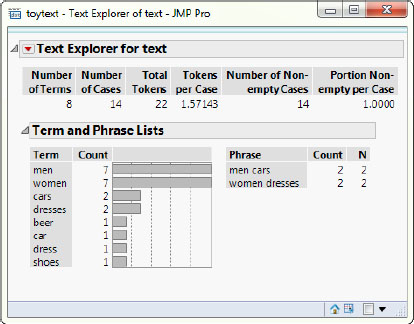
Figure 15.5: Text Explorer Output Box

At the top of Text Explorer output (Figure 15.5), some summary statistics are provided.
Each document is broken into initial units of text called tokens. Usually, a token is a word, but it can be any sequence of non-whitespace characters. As shown in Figure 15.5, there are 22 total tokens.
The basic unit of analysis for text mining is a term. Initially, the Text Explorer examines each of the tokens to determine a possible set of useful terms for analysis. As shown in Figure 15.5, the number of initial terms is 12; they are listed below on the left side and sorted by frequency. This number of terms will change as you transform the text.
On the right side of Figure 15.5, there is a list of phrases common to the corpus—the phrases “men cars” and “women dresses” occurred twice. A phrase is defined as a sequence of tokens that appear more than once. Each phrase will be considered as to whether it should be a term.
Terms are the units of analysis for text mining. Presently, since you have yet to do anything to the data set and if you want to analyze it, complete the following steps:
1. Click the Text Explorer for text red triangle, and select Save Document Term Matrix; accept all the default values.
2. Click OK.
The data table now has 12 new indicator variables, one for each term as shown in Figure 15.6. As you can see in Figure 15.6, one of the first steps that the Text Explorer module does is to convert all the terms to lowercase. In particular, note that dresses and DRESSES are considered as the same term. By default, the Text Explorer also treats the plural of terms, such as dress and dresses or men and man, as different terms or units.
Figure 15.6: Toytext.jmp Data Table with Initial Document Terms

The current number of 14 terms, or indicator variables, is probably more than what you want to work with. You most likely want to combine some of these terms as well as clean up the data before you proceed. (For now, to delete all 12 indicator variables, select all the indicator variable columns, right-click, and click Delete Columns.)
Recode to Correct Misspellings and Group Terms
Examining Figure 15.5 and 15.6 further, you can see that women and woman as well as men and man were not combined. You can also see that there are two misspellings: mn and wn.
To correct the misspelling of mn, click mn in the Text Explorer output, Figure 15.5:
1. Right-click the term mn in the Text Explorer output box and click Recode.
2. As shown in Figure 15.7, in the New Values box, enter men.
3. Click Done.
This misspelling is now included with the term men. The count for men should have increased from 1 to 5. Also, check the data table. Although mn is now included with men within the Text Explorer platform, it is still coded as mn in the data table.
Figure 15.7: Recode Dialog Box

To group together the terms men and man, complete the following steps:
1. Click the term men in the Text Explorer output box, hold down the Ctrl key, and click man.
2. Right-click and click Recode. The Recode dialog box appears.
3. As shown in Figure 15.8, highlight man and men, and right-click.
4. Click Group To men and click Done. The count for men has increased from 2 to 7.
Figure 15.8: The Recode Dialog Box

Similarly, recode wn to women, and group women and woman. The Text Explorer output box will look like Figure 15.9.
Figure 15.9: Text Explorer Output Box
The process of combining related terms is called stemming. Stemming combines related terms with common suffixes—combining words with identical beginnings (called stems), but different endings. To accomplish this, complete the following steps:
1. Click the Text Explorer for text red triangle.
2. Select Term Options ▶ Stemming ▶ Stem for Combining.
The Text Explorer output should look similar to Figure 15.10.
Figure 15.10: Text Explorer Output Box after Stemming

As shown in Figure 15.10, the terms car and cars have been combined into the one new term car⋅ and similarly for dress and dresses. You can check this by clicking one of the stemmed terms car⋅ or dress⋅, right-clicking, and then clicking Show Text.
The recoding of terms thus far completed applies only within the Text Explorer platform; that is, the data is not changed in the data table. To verify, click to open the data table and observe that mn, man, wn, and woman are still listed.
Recoding does affect stemming and should occur before stemming. Hence, it is important that you should try to recode all misspelling and synonyms before executing the Text Explorer platform. Use the Recode procedure under the Cols option. The terms woman dress and man car will also need to be recoded.
Understand the Phrasing Stage
If you want any of the phrases to be analyzed as individual concepts and separated from their individual terms, then you can add these phrases to your term list. For example, to add the phrases men cars and women dresses to your term list, complete the following steps:
1. Click men cars, hold down the Shift key, and click women dresses under the list of Phrases.
2. Right-click, and then click Add Phrase.
The two phrases are now added to the list of terms. They were both stemmed with the plural phrase that appeared only once as shown in Figure 15.11. They are also dimmed in the phrase list, indicating that they are being treated as terms.
Figure 15.11: Text Explorer Output Box after Phrasing

Examining Figure 15.11 further, you can see that the instances of the term men that were in the term men car⋅ have been removed from the count of men and similarly for the term women. To clearly see what you have done so far, complete the following steps:
1. Click the Text Explorer for text red triangle.
2. Select Save Document Term Matrix.
3. Click OK.
Added to the data table are 6 indicator variables, down from your initial 12, one for each term in Figure 15.11, as shown in Figure 15.12.
Figure 15.12: Document Text Matrix

Understand the Terming Stage
Stop words are words that can be characterized in one or more of the following ways:
● too common, such as “a,”, “an,” or “the”;
● infrequent (their counts are low); or
● ignorable (not relevant to the analysis).
Create Stop Words
As shown in Figure 15.11, you have 2 terms with counts of 1. To make them into stop words, complete the following steps:
1. Click beer under the list of Terms.
2. Hold down the Shift key and click shoes.
3. Right-click and then click Add Stop Word.
The list of terms now excludes the terms beer and shoes as shown in Figure 15.13. To see the list of stop words, click the Text Explorer for text red triangle, and select Display Options ▶ Show Stop Words.
Figure 15.13: Text Explorer Output Box after Terming

Generate a Word Cloud
A visualization of the list of terms is called a Word Cloud. To produce the Word Cloud as shown in Figure 15.13, complete the following steps:
1. Click the Text Explorer for text red triangle.
2. Select Display Options ▶ Show Word Cloud.
3. Click the red triangle next to Word Cloud.
4. Select Layout ▶ Centered.
5. Again, click the red triangle next to Word Cloud.
6. Click Coloring ▶ Arbitrary Colors.
The Word Cloud is added to the Text Explorer output as in Figure 15.13. The size of each term in the Word Cloud is relative to its frequency.
Observe the Order of Operations
The list of terms, on the left side of Figure 15.13, shows the list of indicator variables that are used in creating the DTM. As you have worked your way through the flowchart (see Figure 15.2), your objective has been to examine and explore the list of terms and phrases to produce a final list of terms that you are satisfied with. There are no definitive approaches to take, particular words to focus on (depending on the objective of the study and domain expertise), nor a definitive measure to say that you have a good list of terms. This is also an iterative process. However, you should be aware that the order of operation in the creation of a list of terms can affect the resulting list of terms.
The following general steps are suggested:
1. Before executing the Text Explorer, recode all misspellings and synonyms in the data table.
2. In the Text Explorer dialog box, select these options:
a. Minimum number of characters (use 2)
b. Stemming (select Stem for Combining)
c. Tokenizing (select Regex unless you have some custom regexs that you want to add)
3. In the Phrasing Stage, do the following:
a. Examine the phrases.
b. Specify which phrases you want to be included as terms; in particular, select the most frequent sequence of phrases.
4. In the Terming stage, do the following:
a. Remove stop words.
b. Remove least frequent terms.
c. Remove too frequent terms (if any).
Developing the Document Term Matrix with a Larger Data Set
Now you will examine a larger and more realistic data set. The data set traffic_violations_dec2014.jmp contains all the electronic traffic violations that occurred in Montgomery County, Maryland, during December 2014 (dataMontgomery: “All electronic traffic violations”). The file contains 16,446 records and 35 columns. The 35 variables are as follows; their dictionary can be found at (dataMontgomery: “Variable dictionary”):
● Date of Stop
● Time of Stop
● Agency
● SubAgency
● Description
● Location
● Latitude
● Longitude
● Accident
● Belts
● Personal Injury
● Property Damage
● Fatal
● Commercial License
● Hazmat
● Commercial Vehicle
● Alcohol
● Work Zone
● State
● Vehicle Type
● Year
● Make
● Model
● Color
● Violation Type
● Charge
● Article
● Contributed to Accident
● Race
● Gender
● Driver City
● Driver State
● DL State
● Arrest Type
● Geolocation
Generate a Word Cloud and Examine the Text
Examine the text in the variable field Description:
1. Select Analyze ▶ Text Explorer.
2. In the Text Explorer dialog box under 1 Columns, click Description.
3. Click the box Text Columns; change the Minimum Characters per Word to 2.
4. Click the drop-down arrow for Stemming, and choose Stem for Combining.
5. Click OK.
6. In the Text Explorer output, click the Text Explorer for Description red triangle.
7. Click Display Options ▶ Show Word Cloud.
8. Click the red triangle next to Word Cloud,
9. Click Layout ▶ Centered, and again click the red triangle next to Word Cloud.
10. Click Coloring ▶ Arbitrary Colors. The Text Explorer output box with the Word Cloud will appear as shown in Figure 15.14.
Figure 15.14: Text Explorer Output Box

Examine and Group Terms
Under the list of phrases, find the phrase motor vehicle and complete the following steps:
1. Click the phrase motor vehicle.
2. Right-click and then click Select Contains. This option selects bigger phrases that contain this phrase. Scroll down the list of phrases on the right side of the Text Explorer output and you can see highlighted the other phrases that contain the phrase motor vehicle.
Similarly, under the list of phrases, scroll down until you find the phrase driving vehicle on highway and complete the following steps:
1. Click the phrase driving vehicle on highway.
2. Right-click and this time click Select Contained. Scroll up and down the list of phrases; highlighted are all the phrases that contain one or more of the terms in driving vehicle on highway.
As you can see in Figure 15.14, you initially have 741 terms with the terms failure and drive⋅ appearing in a little more than one-third of the documents. (Sometimes, if a term occurs too often, it might not be that usefull; you can make that term a stop word. This will not be considered to be the case here.) Continue with the following steps:
1. Right-click the term failure, and click Show Text. A new window appears, with all the text that contains failure, which appears to be only the term failure.
2. Right-click the term failure, but this time click Containing Phrases. This option selects small phrases that this phrase contains. All the phrases on the right side of Text Explorer output that contain the term failure (which you found to be just the term failure) will be highlighted.
Now examine the term drive⋅ as follows:
1. Click the Text Explorer for Description red triangle.
2. Click Display Options ▶ Show Stem Report. Added to the Text Explorer output are two lists—on the left, a list of stemmed terms and their terms used in the stem and, on the right, the list of terms and the term that they are stemmed with.
3. Scroll down the left, until you come to drive⋅ (stemmed terms are in alphabetic order). You can see the terms associated with the stemmed term drive⋅ are drive and driving.
(Note that if there is one or more stemmings that you do not like, it is probably best to exit the Text Explorer. Recode those undesired stemmings, and restart the Text Explorer.)
Add Frequent Phrases to List of Terms
Next add the most frequent phrases to your list of terms. Arbitrarily, you decide to include all the phrases occurring more than 500 times.
1. Click the first phrase under the list of phrases, which is driver failure.
2. Hold down the Shift key, scroll down, and click the phrase influence of alcohol. Notice that all the phrases above are now highlighted.
3. Right-click and click Add Phrase.
Several changes occur, and the Text Explorer output will look as shown in Figure 15.15.
Figure 15.15: Text Explorer Output Box

Parse the List of Terms
Lastly, parse your list of terms:
1. Right-click anywhere under the list of terms and, in the list of options, click Alphabetic Order.
2. Click the first term 1; hold down the Shift key, and scroll down to and click 99.
3. Right-click and click Add Stop Word. All these number terms are now deleted from your list of terms.
4. Again, right-click under the list of terms, and deselect Alphabetic Order. As before, the terms are now sorted by frequency.
Now delete all the terms that occur fewer than 100 times:
1. Scroll down the list of terms until you come to the term secur⋅, which occurs 97 times.
2. Click secur⋅; hold down the Shift key, scroll down to the end, and click vehicle on highway without.
3. Right-click and click Add Stop Word.
The Text Explorer output will now look similar to Figure 15.16.
Figure 15.16: Text Explorer Output Box

Using Multivariate Techniques
After you have curated the DTM to your satisfaction, you are ready to apply multivariate techniques to understand the underlying structure of the DTM.
These techniques are similar to principal components, factor analysis, and clustering techniques that are applied to continuous data.
Perform Latent Semantic Analysis
Latent Semantic Analysis (LSA) is a family of mathematical and statistical techniques for extracting and representing the terms and phrases from a corpus. The DTM is reduced dimensionally to a manageable size, which makes the analyses go much faster. And the DTM is amenable to using other multivariate techniques, by applying singular value decomposition (SVD).
Understanding SVD Matrices
SVD produces a set of orthogonal columns that are linear combinations of the rows and explains as much of the variation of the data as possible. SVD is an efficient approach to use with large, very sparse matrices, which the DTM typically tends to have. SVD decomposes the DTM into three other matrices:
DTM = D * S * T
These matrices are defined as follows:
● D is an orthogonal document-document matrix of eigenvectors.
● T is an orthogonal term-term matrix of eigenvectors.
● S is a diagonal matrix of singular values.
The singular vectors in D and T reveal document-document, document-term, and term-term similarities and other semantic relationships, which otherwise might be hidden.
Many of the singular values in the S matrix are “too small” and can be ignored. So they are assigned values of 0, leaving k nonzero singular values. The representation of the conceptual space of any large corpus requires more than a handful of underlying independent concepts. As a result, the number of orthogonal vectors that is needed is likely to be fairly large. So, k is often several hundred.
Similarities and relationships are now approximated by this reduced model. This process is analogous to using principal components in multivariate analysis. While principal components provide components for the columns, SVD simultaneously provides principal components for both the columns and rows (that is, for the documents and terms).
Plot the Documents or Terms
A common practice is to plot the documents or terms, these singular vectors, and especially the first two vectors, that result from the SVD. Similar documents or terms tend to be plotted closely together, and a rough interpretation can be assigned to the dimensions that appear in the plot. Complete the following steps:
1. Click the Text Explorer for Description red triangle, and click Latent Semantic Analysis, SVD. The Latent Semantic Analysis Specifications dialog box will appear as shown in Figure 15.17.
2. Change the Minimum Term Frequency to 100.
3. Click the drop-down arrow for Weighting.
4. The TF_IDF weighting results are usually more interpretable than the Binary, so click that option.
Regarding weighting options, various methods of the term-frequency counts have been found to be useful, with the Binary and TF_IDF being the most popular:
● The Binary weighting option is the easiest to understand in that it assigns a zero or a 1 to indicate whether the term exists in the document. A disadvantage of the Binary option is that it does not consider how often the term occurs in the document.
● The TF_IDF weighting option, which is short for term frequency–inverse document frequency, does consider the tradeoff between the frequency of the term throughout the corpus and the frequency of the term in the document.
Next you will select one of three SVD approaches:
● Uncentered
● Centered
● Centered and Scaled
The benefits and drawbacks of each are as follows:
● Traditional latent semantic analysis uses an Uncentered approach. This approach can be problematic because frequent terms that do not contribute much meaning tend to score high in the singular vectors.
● The Centered approach reduces the impact of these frequent terms and reduces the need to use many stop words.
● The Centered and Scaling approach is essentially equivalent to doing principal components on the correlation matrix of the DTM. This option explains the variation in the data (not just the variation in the mean). Therefore, it tends to produce more useful results, whereas using just the Centered approach is comparable to doing principal components on the covariance matrix of the DTM.
Continue with the example as follows:
1. Click the drop-down arrow for Centering and Scaling. Select the Centered and Scaling approach.
2. Click OK.
Figure 15.17: Latent Semantic Analysis Specifications Dialog Box

The Latent Semantic Analysis output should look similar to Figure 15.18 (except for the highlighted regions).
Figure 15.18: SVD Plots

The plot on the left displays the first two document singular vectors in matrix D. The plot on the right displays the first term singular vectors in T as shown in Figure 15.18. In each graph, the singular vectors have three branches or tendrils. In the document singular vector graph, the three tendrils are highlighted and labeled. To examine the text, complete the following steps:
1. Left-click the document singular vector graph, hold down the mouse button, and move to highlight the area labelled 1 in Figure 15.18.
2. Just below SVD plots, click Show Text. A window appears with a list of documents.
Examining the document list, you see that major themes are the drive use handheld and failure of vehicle on highway to display lighted lamps.
Similarly, highlight, the documents in the tendril labeled 2 and click Show Text. These documents appear to have several themes of driving vehicle, person drive motor vehicle, and negligent driving. Lastly, highlight the documents in Tendril 3, and you see the terms driving vehicle on highway without current registration and failure of licensee to notify. (Keep these documents in the third tendril highlighted.)
As you did with the document singular vectors, you can explore the term three tendrils in the term singular vector plot. In general, the document singular vector plot provides more insight than the term singular vector plot.
To examine more SVD plots, complete the following steps:
1. Click the Text Explorer for Description red triangle.
2. Click SVD Scatterplot Matrix.
3. Enter 10 for the Number of singular vectors to plot.
4. Click OK.
Added to the Text Explorer output are scatterplots of the first 10 singular vectors for the documents and terms. Figure 15.19 shows the top part of this scatterplot.
Figure 15.19: Top Portion of SVD Scatterplots of SVD Plots of 10 Singular Vectors

The bottom diagonal plots are graphs of the document singular vectors. The upper diagonal plots are graphs of the term singular vectors. Highlighted in Figure 15.19 is the SVD plot of the first two document singular vectors, which is similar to the plot on the left in Figure 15.18. The highlighted documents in the third tendril are highlighted. And these documents are highlighted in the other document singular vector plots. The term singular vector plot directly above the highlighted document singular vector plot in Figure 15.19 is the plot of the first two-term singular vectors, which is similar to the plot in Figure 15.18 but rotated 270°.
Perform Topic Analysis
Another way of observing these term themes in the documents is to perform topic analysis. Topic analysis performs a VARIMAX rotation, essentially a factor analysis, on the SVD of the DTM. Complete the following steps:
1. Click the red triangle next to Text Explorer for Description.
2. From the list options click Topic Analysis, Rotated SVD.
3. Click OK.
The Topic Analysis results are added to the Text Explorer output as shown Figure 15.20.
Figure 15.20: Topic Analysis Output

The scores represent the loading of the term in that topic. The larger a term’s score, the stronger its contribution to the topic. Each topic can be examined for major themes or terms that contribute to that topic. In particular, when you examine the first topic in Figure 15.20, it appears that this topic deals with careless and negligent, somewhat like Tendril 2, which you identified in the SVD plots. And topic 2 seems to have similar terms as Tendril 1. If you choose to consider too few topics, then there can be significant overlap between competing information. But if you choose too many topics, then you will have some topics covering the same topics. Use trial and error to decide how many to consider.
Perform Cluster Analysis
Cluster analysis is used to further understand the singular vectors. The Text Explorer platform in JMP uses a customized latent class analysis methodology for cluster analysis. This is built just for text. This latent class analysis procedure is good for finding interesting patterns in the text, and because it is sparse matrix based, it is very fast.
Begin the Analysis
To begin, complete the following steps:
1. Click the red triangle next to Text Explorer for Description and click Latent Class Analysis.
2. In the Specifications dialog box, change the Minimum Term Frequency to 4 and the Number of Clusters to 10.
3. Click OK.
4. Click the red triangle labelled Latent Class Analysis for 10 Clusters and click Color by Cluster.
The cluster analysis results are shown in Figures 15.21 and 15.22. Because the latent class analysis procedure uses a random seed, your results will be slightly different.
Examine the Results
Scroll back up to the SVD scatterplots. The document SVD plots are now colored by cluster. Documents that tend to cluster together will appear near each other in their SVD plots. (You can increase the size of a plot by grabbing the border with the mouse while holding down the mouse key and dragging out wider.) For example, in Figure 15.23 the upper left portion of the SVD scatterplot is shown.
Look at the group of documents highlighted in Doc Vec3. All these documents are in the same cluster and in other plots. You can see that they are close to each other. Match up the color of these documents with cluster colors as shown in Figure 15.21. Click that cluster number; in our case it was Cluster 6. Now all the documents in Cluster 6 are highlighted in the SVD scatterplots.
Scroll further up to SVD Plots. In the left document singular vector plot, the Cluster 6 documents are highlighted, which are mostly those documents in Tendril 3 (as shown in Figure 15.18). Click Show Text. You see phrases or terms similar to those that you found in Tendril 3. Similarly, you can highlight other clusters of the same colored documents and view the text.
Figure 15.21: Top Portion of Latent Class Analysis for 10 Clusters Output Box

Figure 15.22: Lower Portion of Latent Class Analysis for 10 Clusters Output Box

Figure 15.23: Upper Leftmost Portion of SVD Scatterplots

Identify Dominant Terms
The Term Probabilities by Cluster report in Figure 15.21 has the term frequency in each cluster. You can examine the terms horizontally or the clusters vertically, focusing on the large frequencies. For example, look at the term license, which occurs most often in Clusters 6 and 7. Since you previously have looked at Cluster 6, look at Cluster 7:
1. Right-click anywhere inside the report.
2. Select Sort Column.
3. In the new window, select Cluster 7.
4. Click OK.
The most frequent terms in Cluster 7 are toward the top of the report. It seems that the Cluster 7 theme addresses drivers who were driving with suspended licenses.
A scoring algorithm for identifying which terms are most dominant within a cluster is shown in the Top Terms per Cluster report (see Figure 15.21). The score is based on the term cluster frequency relative to its corpus frequency. Larger scores tend to occur more often in the cluster. Look at Cluster 6 and 7. You see the most frequent terms are the terms you have identified earlier.
Occasionally terms score negative numbers, which implies that those terms are less frequent (you do not have any negative scores in our example). Many times when several terms have negative numbers, they occur in the same cluster. This is called a junk cluster. Most likely in this junk cluster are blank documents or simply documents that do not fit nicely in other clusters and just are adding noise to the analysis. If a junk cluster occurs, then it may be useful to identify those documents in this cluster and rerun latent class analysis to exclude these junk documents.
The multiple dimensional scaling (MDS) plot of the clusters in Figure 15.22 is produced by calculating the Kullback-Leibler distance between clusters. In natural language processing (NLP), a document is viewed as a probability distribution of terms. The Kullback-Leibler distance is a widely used measure for calculating the distance between two documents or probability distributions (Bigi). An MDS is applied to these Kullback-Leibler distances to create coordinates for the clustering in two dimensions. You can explore the MDS plot to examine clusters that are near one another, as well as clusters that are far away from one another.
The clusters in your MDS plot are fairly well dispersed. Nonetheless, complete the following steps:
1. Click Cluster 3. You can see in the Top Terms per Cluster report that the main terms are driver⋅ failure to obey, devic⋅ instructions, and proper⋅ placed traffic control⋅.
2. Scroll back up to the output. You can see where the Cluster 3 documents occur in the SVD plots.
3. Click Show text.
Most of the documents appear to have those terms that you detected.
Using Predictive Techniques
If the data set has a dependent variable and you want to do some predictive modeling instead of using the large DTM matrix, you can use the document singular vectors. To determine how many singular vectors to include, complete the following steps:
1. Scroll back up the output to find Singular Values. (It is just below the SVD plots and before the SVD Scatterplots.)
2. Click the down-arrow next to Singular Values.
In general, as in principal components and factor analysis, you are looking for the elbow in the data. Or another guideline is to include singular values until you reach a cumulative percentage of 80%. Many times with text data, the curve or percentages will only gradually decrease, so to reach 80% you may have to reach several hundred. As you will see, the default is 100. How many to include is a judgment call.
Figure 15.24 shows the first 25 singular values. In this case, the percentages quickly exceed 80%, and there is a sharp decrease. Six singular document vectors are chosen:
1. Click the Text Explorer for Description red triangle.
2. Click Save Document Singular Vectors.
3. In the input box in the new dialog box next to Number of Singular Vectors to Save, enter 6.
4. Click OK.
Check the data table, and you can see six new singular vector variables.
Figure 15.24: Singular Values

Perform Primary Analysis
Before you perform any predictive modeling, do some primary analysis:
1. Click Analyze ▶ Distribution. The distribution dialog box will appear.
2. Click Violation Type; click Y, Columns.
3. Click OK.
As shown in the distribution output in Figure 15.25, you can see that most of the violations are equally distributed between Warning and Citation.
Figure 15.25: Distribution Output for Violation Type

Perform Logistic Regressions
Now run a logistic regression, predicting Violation Type and using Property Damage, Race, and Belts as independent variables. The results are shown in Figures 15.26 and 15.27. You can see that the three variables are significant in predicting Violation Type. However, as the Confusion matrix in Figure 15.27 shows, the misclassification is rather high at 47.6%.
Figure 15.26: Top Portion of Initial Logistic Regression Output

Figure 15.27: Lower Portion of Initial Logistic Regression Output

Rerun the logistic regression, now also including the six singular vectors. Figures 15.28 and 15.29 display the output. The model significantly improved and now has a misclassification rate of 40.7% (not great, but almost 7% better).
Figure 15.28: Top Portion with Singular Values Logistic Regression Output

Figure 15.29: Lower Portion with Singular Values Logistic Regression Output

Exercises
1. In the aircraft_incidents.jmp file is data for airline incidents that were retrieved on November 20th, 2015 from http://www.ntsb.gov/_layouts/ntsb.aviation/Index.aspx. For the Final Narrative variable, use the Text Explorer to produce a DTM by phrasing and terming.
2. Create a Word Cloud. As in problem 1, similarly produce a DTM by phrasing and terming, and create a Word Cloud except for the variable Narrative Cause. In the file Nicardipine.jmp is data from adverse events from this drug. For the Reported Term for the Adverse Event variable, use the Text Explorer to produce a DTM by phrasing and terming.
3. Create a Word Cloud. In the Airplane_Crash_Reports.jmp file is one variable, NTSB Narrative, that summarizes the crash report. For this variable, use the Text Explorer to produce a DTM by phrasing and terming.
4. Create a Word Cloud. In the FDA_Enforcement_Actions.jmp file, the variable Citation Description describes the violation. For this variable, use the Text Explorer to produce a DTM by phrasing and terming.
5. Create a Word Cloud. The traffic-violation_jun2015.jmp is similar to the file used in the chapter except that the data is for June 2015 only. For the variable Description, use the Text Explorer to produce a DTM by phrasing and terming.
6. Create a Word Cloud. How does this compare to data for December 2014? Perform Latent Semantic Analytics, Topic Analysis, and Cluster Analysis on the DTM you produced in Problem 1. Perform Latent Semantic Analytics, Topic Analysis, and Cluster Analysis on the DTM you produced in Problem 2.
7. Perform Latent Semantic Analytics, Topic Analysis, and Cluster Analysis on the DTM that you produced in Problem 3. Perform Latent Semantic Analytics, Topic Analysis, and Cluster Analysis on the DTM you produced in Problem 4. Perform Latent Semantic Analytics, Topic Analysis, and Cluster Analysis on the DTM you produced in Problem 5. Perform Latent Semantic Analytics, Topic Analysis, and Cluster Analysis on the DTM you produced in Problem 6. How does this compare to data for December 2014?
8. Similar to the predictive model that you did in the chapter, create a predictive model for violation type. How does this compare to data for December 2014?
1 The authors would like to thank Daniel Valente and Christopher Gotwalt for their guidance and insight in writing this chapter.