Appendix B
Autocorrelation and Partial Autocorrelation
B.1. Partial Autocorrelation
B.1.1 Computation Algorithm
From the autocorrelations ρ X (1), …, ρ X (h), the partial autocorrelation r X (h) can be computed rapidly with the aid of Durbin's algorithm:

Steps (B.8) and (B.9) are repeated for k = 2, …, h − 1, and then r X (h) = a h, h is obtained by step (B.8); see Exercise 1.14.
B.1.2 Behaviour of the Empirical Partial Autocorrelation
The empirical partial autocorrelation, ![]() , is obtained from the algorithm (B.7)–(B.9), replacing the theoretical autocorrelations
ρ
X
(k) by the empirical autocorrelations
, is obtained from the algorithm (B.7)–(B.9), replacing the theoretical autocorrelations
ρ
X
(k) by the empirical autocorrelations ![]() , defined by
, defined by
for
h = 0, 1, …, n − 1. When (X
t
) is not assumed to be centred,
X
t
is replaced by ![]() . In view of (B.5), we know that, for an AR(p) process, we have
r
X
(h) = 0, for all
h > p
. When the noise is strong, the asymptotic distribution of the
. In view of (B.5), we know that, for an AR(p) process, we have
r
X
(h) = 0, for all
h > p
. When the noise is strong, the asymptotic distribution of the ![]() ,
h > p
, is quite simple.
,
h > p
, is quite simple.
It follows that for a GARCH, and more generally for a weak white noise, ![]() and
and ![]() have the same asymptotic distribution.
have the same asymptotic distribution.
The following result is stronger because it shows that, for a white noise, ![]() and
and ![]() are asymptotically equivalent.
are asymptotically equivalent.
B.2. Generalised Bartlett Formula for Non‐linear Processes
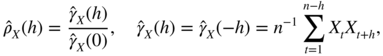
Let X 1, …, X n be observations of a centred second‐order stationary process X = (X t ). The empirical autocovariances and autocorrelations are defined by

for h = 0, …, n − 1. The following theorem provides an expression for the asymptotic variance of these estimators. This expression, which will be called Bartlett's formula, is relatively easy to compute. For the empirical autocorrelations of (strongly) linear processes, we obtain the standard Bartlett formula, involving only the theoretical autocorrelation function of the observed process. For non‐linear processes admitting a weakly linear representation, the generalised Bartlett formula involves the autocorrelation function of the observed process, the kurtosis of the linear innovation process, and the autocorrelation function of its square. This formula is obtained under a symmetry assumption on the linear innovation process.