Chapter 5: Running Machine Learning Jobs on Elasticsearch

In the previous chapter, we looked at how large volumes of data can be managed and leveraged for analytical insight. We looked at how changes in data can be detected and responded to using rules (also called alerts). This chapter explores the use of machine learning techniques to look for unknowns in data and understand trends that cannot be captured using a rule-based approach.

Machine learning is a dense subject with a wide range of theoretical and practical concepts to cover. In this chapter, we will focus on some of the more important aspects of running machine learning jobs on Elasticsearch. Specifically, we will cover the following:

• Preparing data for machine learning
• Running single- and multi-metric anomaly detection jobs on time series data
• Classifying data using supervised machine learning models
• Running machine learning inference on incoming data

Technical requirements

To use machine learning features, ensure that the Elasticsearch cluster contains at least one node with the role ml. This enables the running of machine learning jobs on the cluster:

• If you're running with default settings on a single node, this role should already be enabled, and no further configuration is necessary.
• If you're running nodes with custom roles, ensure the role is added to elasticsearch.yml, as follows:

  node.roles: [data, ml]

The value of running machine learning on Elasticsearch

Elasticsearch is a powerful tool when it comes to storing, searching, and aggregating large volumes of data. Dashboards and visualizations help with user-driven interrogation and exploration of data, while tools such as Watcher and Kibana alerting allow users to take automatic action when data changes in a predefined or expected manner.

However, a lot of data sources can often represent trends or insights that are hard to capture as a predefined rule or query. Consider the following example:

• A logging platform collects application logs (using an agent) from about 5,000 endpoints across an environment.
• The application generates a log line for every transaction executed as soon as the transaction completes.
• After a software patch, a small subset of the endpoints can intermittently and temporarily fail to write logs successfully. The machine doesn't entirely fail as the failure is intermittent in nature.
• While the platform does see a drop in overall log volume throughput, it is not drastic enough to trigger a predefined alert or catch the eye of the platform operator.

This sort of failure can be very hard to detect using standard alerting logic but can be extremely easy to spot when using anomaly detection. Machine learning models can build a baseline for log volumes per data source over a period of time (or a season), learning the normal changes and variations in volumes. If a failure was to occur, the new values observed would fall outside the expected range on the model, resulting in an anomaly.

Consider a slightly different example (and one that we will use in subsequent sections of this chapter).

A web server logs all requests made to an internet-facing web application. The application is used by various employees who are working from home (and therefore outside the company network) and administrators who look after the system. The logs look as follows:

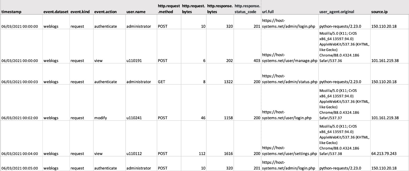
Figure 5.1 – Sample logs from a web application

Navigate to Chapter5/dataset in the code repository and ingest the web application logs into your Elasticsearch cluster, as follows:

1. Load the index template and ingest a pipeline by running load.sh. Enter your Elasticsearch cluster URL, username, and password when prompted:

   ./load.sh

2. Update webapp-logstash.conf with the appropriate Elasticsearch cluster credentials and use Logstash to ingest the webapp.csv file:

   logstash-8.0.0/bin/logstash -f webapp-logstash.conf < webapp.csv

3. Confirm the data is available on Elasticsearch:

   GET webapp/_search

Here is the output:

Figure 5.2 – Stats from the webapp index

4. Create a data view on Kibana for the webapp index:
   1. On Kibana, open the navigation menu on the top left and navigate to Stack Management.
   2. Click on Data Views under the Kibana section and click on Create data view.
   3. Type in webapp as the name of the data view and click Next step.

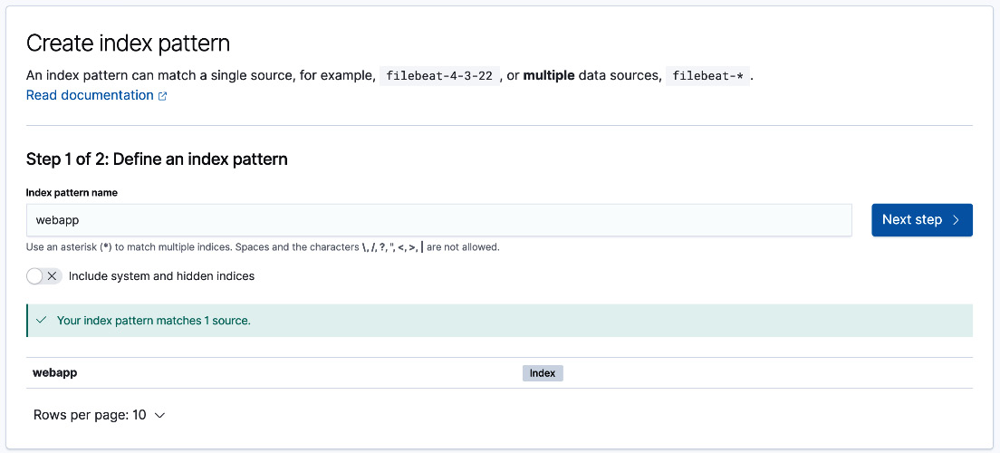
Figure 5.3 – Create data view on Kibana

4. Select @timestamp as the time field and click on Create data view.

Data views on Kibana map to one or more indices on Elasticsearch and provide Kibana with information on fields and mappings to enable visualization features. We will further explore Kibana concepts and functionality in Chapter 8, Interacting with Your Data on Kibana.

Open up the Discover app from the navigation menu and click on the calendar icon to select a time range for your data. This dataset in particular contains events from March 6, 2021 to March 11, 2021. Click on the Update button once selected to view your data.

Figure 5.4 – webapp documents on Discover

The next section looks at preparing data for use in machine learning jobs.

Preparing data for machine learning jobs

In order for machine learning jobs to analyze document field values when building baselines and identifying anomalies, it is important to ensure the index mappings are accurately defined. Furthermore, it is useful to parse out complex fields (using ETL tools or ingest pipelines) into their own subfields to use in machine learning jobs.

The machine learning application provides useful functionality to visualize the index you're looking to run jobs on, and ensure mappings and values are as expected. The UI lists all fields, data types, and some sample values where appropriate.

Navigate to the machine learning app on Kibana and perform the following steps:

1. Click on the Data Visualizer tab.
2. Select the webapp data view you created in the previous section.
3. Click on Use full webapp data to automatically update the time range filter for the full duration of your dataset.
4. Inspect the fields in the index and confirm all fields are mapped as expected. Explore the values and distribution of textual fields and the statistical summaries of numeric fields to understand how you may structure your machine learning jobs.

Figure 5.5 – Data Visualizer UI on the machine learning app

Now that we've prepared our dataset, let's look at some core machine learning concepts that make up the capabilities of the Elastic Stack.

Machine learning concepts

The machine learning technique or approach you use depends on the data and use case you're looking to solve; it comes down to the question you're asking of your data. Broadly, the approaches can be broken down into the following.

Unsupervised learning

Unsupervised learning is a machine learning approach that learns patterns and trends in data without any external labeling or tagging. The approach can be used to extract otherwise hard-to-find behaviors in the data without human intervention.

At a high level, the technique works by analyzing functions of field values (over time, or a series of documents) to build a behavior baseline (a norm). New field values are compared to the baseline, including a margin of error. Data points that fall outside the expected range are classified as anomalies. Assuming the model has analyzed sufficient data to capture the seasonality of the dataset, it can also be used to forecast values for fields in future time ranges.

Some use cases for unsupervised learning include the following:

• Identifying unexpected changes in metric data
• Detecting erratic behavior without the use of rigid thresholds
• Unknown security threats that may not have a predefined detection rule

The Elastic Stack implements the aforementioned unsupervised learning use cases as part of the time series anomaly detection and outlier detection features.

Supervised learning

Supervised learning is an approach where a machine learning model is trained with labeled training data that tells the algorithm about an outcome or observed value, given the input data. The approach is useful when you know the input and output to a given problem, but not necessarily how to solve it.

Supervised learning works by analyzing key features and the corresponding output value in a dataset and producing a mapping for them. This mapping can then be used to predict output values given new and unseen inputs.

Examples of use cases that can leverage supervised learning include the following:

• Flagging/classifying fraudulent transactions on your application from audit logs
• Predicting the probability of a customer churning (or leaving the company) given current usage patterns
• Identifying potentially malicious activity or abuse from activity logs

The Data Frame Analytics tab on the machine learning app offers classification (to predict or classify data into categories) and regression (predicting values for fields based on their relationships) as supervised learning features.

Next, we will look at how machine learning can be used to detect anomalies in time series datasets.

Looking for anomalies in time series data

Given the logs in the webapp index, there is some concern that there was some potentially undesired activity happening on the application. This could be completely benign or have malicious consequences. This section will look at how a series of machine learning jobs can be implemented to better understand and analyze the activity in the logs.

Looking for anomalous event rates in application logs

We will use a single-metric machine learning job to build a baseline for the number of log events generated by the application during normal operation.

Follow these steps to configure the job:

1. Open the machine learning app from the navigation menu and click on the Anomaly Detection tab.
2. Click on Create job and select the webapp data view. You could optionally use a saved search here with predefined filters applied to narrow down the data used for the job.
3. Create a single-metric job as we're only interested in the event rate as we start the analysis.
4. Use the full webapp data and click on Next.
5. Select Count(Event Rate) in the dropdown. The Count function will take into account both high and low count anomalies, both of which are interesting from an analysis perspective. The reference guide contains more information on all of the functions available to use: https://www.elastic.co/guide/en/machine-learning/8.0/ml-functions.html.
6. The bucket span determines how the time series data is grouped for analysis. A smaller bucket span will result in more granular analysis with a large number of buckets (and therefore more compute/memory resources required to process). A larger bucket span means larger groups of events, where less extreme anomalies may be suppressed. The UI can estimate an ideal bucket span for you. In this example, we will use a bucket span of 1 minute (1m). Click on Next.
7. Provide a job ID on the form (a unique identifier for the job). The example uses the event-rate-1m ID. Click Next.
8. Assuming your configuration passes validation, click Next.
9. Review the job configuration summary and click on Create Job.
10. The job will take a few seconds to run (longer on bigger, real-world datasets). Progress will be shown on the UI as it runs.

Figure 5.6 – Single-metric job summary

11. Click on the View results button to open the metric viewer window to explore trends in the data.

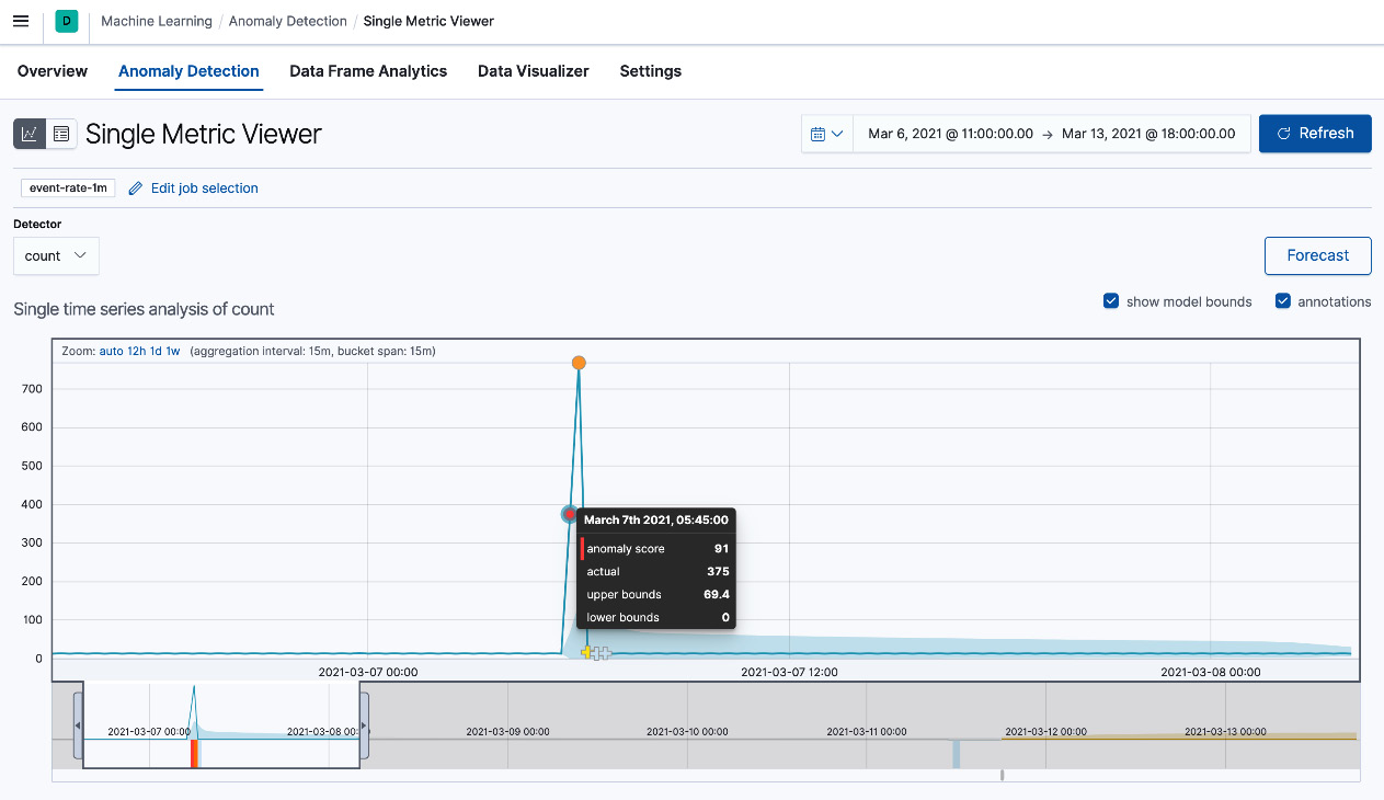
Figure 5.7 – Single Metric Viewer UI

The chart displays the following information:

• The solid line displays the variation in the metric (the event rate) being analyzed.
• Annotations represented by circles show any anomalies that were detected for any given bucket. The annotation displays the time bucket that the anomaly occurred in, a score, the actual value observed, and upper/lower bounds.
• The blue area graph shows the margin of error for anomalies based on observed values.
• The table below the chart shows details of the anomalies detected. The information includes the score, the type of anomaly detector used (count in this case), observed versus expected values, and a description quantifying the difference between the observed/expected values.

Figure 5.8 – Tabular view of anomalies

Given the information from this job, we can come to the following conclusions:

• The event rate on the system is mostly very consistent.
• There was a drastic spike in events starting on March 7, 2021, at 05:30. This resulted in the detection of two strong anomalies. At its peak, the event rate was 38x higher than its normal value.
• The anomalous event spike subsided within an hour, with activity returning to normal for the rest of the time period. No low-count anomalies were detected, indicating the availability of the application was unaffected after the spike.

Looking for anomalous data transfer volumes

We know that the previous job indicated an unexpected and anomalous spike in the number of requests received by the web app (event rate). One option to further understand the implications of this activity is to analyze the amount of data sent and received by the application. We will use a multi-metric anomaly detection job to achieve this outcome.

Follow these instructions to configure the job:

1. Click on Create job on the Anomaly Detection tab.
2. Select the webapp data view and click Next.
3. Create a multi-metric job so we can analyze the number of bytes sent and received by the application.
4. Use the full webapp data and click Next.
5. Select Mean(http.request.bytes) in the Add metric drop-down box. We use the mean function here as we are interested in the anomalous nature of individual transactions. In another job, you could also analyze the sum of this metric to detect anomalous patterns using many normal-looking transactions.
6. Also select Mean(http.response.bytes) from the same drop-down box.
7. A split field could be used to partition the dataset and model each subset independently. Select url.path to analyze access patterns for each application path separately.
8. Influencers are fields that might have an effect on the metric(s) being analyzed. As such, these fields can usually provide context to an anomaly and are useful to assign blame for an outcome. From the Influencers dropdown, select the following:
   1. url.path
   2. source.ip
   3. source.geo.country_name
9. Use a bucket span of 2m for the job and click on Next to continue.
10. Provide a job ID and continue. The example uses the bytes-in-out ID.
11. Assuming your job passes validation, continue to the next screen.
12. Click on Create Job to start the analysis. Your screen should look as follows:

Figure 5.9 – Multi-metric job summary

13. Click on View results to open the Anomaly Explorer interface. The heatmap displays anomaly scores for a given time bucket, broken down by an influencer value (as per the job configuration). The following screenshot displays anomalies grouped by the url.path field. This can be changed during analysis using the drop-down box:

Figure 5.10 – Anomaly Explorer for a multi-metric job

14. The table below the heat map lists all identified anomalies, including the detector used, the values of influencer fields, and actual and typical values.

Figure 5.11 – Tabular view of anomalies

From the results produced by the completed machine learning job, we can make the following observations and conclusions:

• Anomalous data transfer volumes were first observed on admin/login.php, where volumes were more than 100x higher than expected. Traffic was seen from a single source.ip address with a geo-location in Malaysia (which happens to be outside the normal and expected geo-locations for this application).
• The same source IP address was later seen interacting with user/customer.php and user/order.php with anomalous data transfer volumes (64x higher than expected) compared to all other source IP addresses in the environment (as shown by the following graph):

  Note

  The following graphs can be viewed by clicking on a cell in the anomaly timeline heatmap on the Kibana interface.

Figure 5.12 – Charts displaying values for individual metrics

• The anomalous activity continued for a brief period of time on 2 consecutive days after initial activity, with similarly high-volume traffic patterns.
• When analyzing the event rate in the previous job, there was only one big spike in events, around the time when admin/login.php saw high volumes. This means that the high volumes seen on the latter URL paths (such as user/customer.php and user/order.php) were through a small number of transactions.
• This would indicate that an unauthorized user (from a singular source IP address) likely gained access to the application (from the initial spike in events) and subsequently sent requests to download large amounts of data.

Comparing the behavior of source IP addresses against the population

We've detected anomalies in overall event rates as well as data transfer volumes for different URL paths on the web app. From the second job, it was evident that a lot of the anomalies originated from a singular IP address. This leads to the question of how anomalous the activity originating from this IP address was, compared to the rest of the source IP addresses in the dataset (or population of source IPs). We will use a population job to analyze this activity.

Follow these instructions to configure this job:

1. Create a new population anomaly detection job using the webapp data view.
2. Use the entire time range for the data and continue.
3. The Population field can be used to group related data together. We will use source.ip as the population field so we treat all traffic originating from the same IP address as related.
4. Select Count(Event Rate) as your first metric to detect any source IPs producing too many events compared to the rest of the population.
5. Select Mean(http.request.bytes) and Mean(http.response.bytes) to track anomalous data transfer volumes and click Next to continue.
6. Select source.geo.country_name and user_agent.name as influencers, in addition to the automatically added source.ip field.
7. Provide a job ID and continue. The example uses population-source-ip.
8. Click Next to see the summary and run the job.

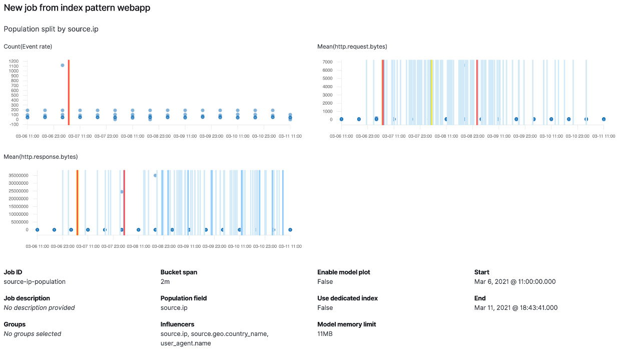
Figure 5.13 – Population job summary

9. View results on the Anomaly Explorer page to analyze the results.

Figure 5.14 – Anomaly Explorer heat map for the population job

As expected, there is a singular source IP that stands out with anomalous activity, both in terms of event rate and data transfer volumes compared to the rest of the population.

You can also view it by the user_agent.name value and see that most of the anomalous requests came from curl and a version of Firefox.

Figure 5.15 – Anomaly heatmap viewed by user agent

From looking at the anomalies detected, we can conclude the following:

• A singular source IP address in Malaysia was responsible for most of the anomalous activity on the system.
• Two distinct user_agent values were observed (from the same IP address).
• All other source IP addresses in the population had fairly uniform behavior compared to the IP 210.19.10.10.

Now that we have gathered enough data, we can use the Discover tab to explore the raw events. Type the following query into the search bar to filter for HTTP 200 response codes for successful authentication requests and remove the noise from any failed authentication requests:

source.ip: "210.19.10.10" AND (http.response.status_code : "200" OR http.response.status_code:"201")

We can now see the events from the potentially malicious IP address successfully authenticating with the application and exfiltrating customer data over the course of 3 days.

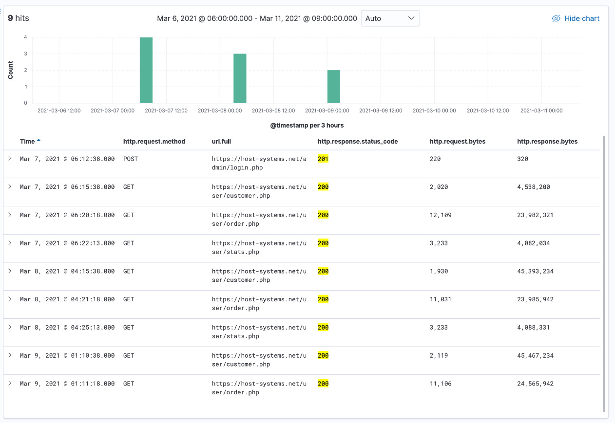
Figure 5.16 – Raw events upon discovering the record displaying malicious activity

Now that we know how various types of unsupervised anomaly detection jobs can be used in analyzing logs, the next section will focus on using supervised machine learning to train models and classify your data.

Running classification on data

Unsupervised anomaly detection is useful when looking for abnormal or unexpected behavior in a dataset to guide investigation and analysis. It can unearth silent faults, unexpected usage patterns, resource abuse, or malicious user activity. This is just one class of use cases enabled by machine learning.

It is common to have historical data where, with post analysis, it is rather easy to label or tag this data with a meaningful value. For example, if you have access to service usage data for your subscription-based online application along with a record of canceled subscriptions, you could tag snapshots of the usage activity with a label indicating whether the customer churned.

Consider a different example where an IT team has access to web application logs where, with post analysis, given the request payloads are different to normal requests originating from the application, they can label events that indicate malicious activity, such as password spraying attempts (as the request payloads are different to normal requests originating from the application).

Training a machine learning model with input data and a labeled outcome (did the customer churn, or was the request maliciously crafted?) is a useful tool for taking proactive and timely data-driven action. Users likely to churn can be offered a discount on the service or access to tutorials so they can leverage the service better. IP addresses responsible for maliciously crafted requests can be blocked proactively without manual intervention, and the security team can be alerted to take broader action (such as enforcing two-factor authentication or asking users to change their passwords).

Data frame analytics on elastic machine learning provides two main features to help with such use cases:

• Regression: Used to predict scalar values for fields (such as estimated air ticket prices for a given route/date or how much a user would like a given movie)
• Classification: Used to predict what category a given event would fall under (such as determining whether payloads indicate a maliciously crafted request or a borrower is likely to pay back their debt on time)

Predicting maliciously crafted requests using classification

We will implement a classification job to analyze features in web application requests to predict whether a request is malicious in nature. Looking at the nature of the requests as well as some of the findings from the anomaly detection jobs, we know that request/response sizes for malicious requests are not the same as the standard, user-generated requests.

Before configuring the job, follow these steps to ingest a tagged dataset where an additional malicious Boolean column is introduced to the CSV file:

1. Update webapp-tagged-logstash.conf with the appropriate Elasticsearch cluster credentials and use Logstash to ingest the webapp-tagged.csv file:

   logstash-8.0.0/bin/logstash -f webapp-tagged-logstash.conf < webapp-tagged.csv

2. Confirm the data is available on Elasticsearch:

   GET webapp-tagged/_search

3. Create a data view on Kibana (as shown in the previous section) for the webapp-tagged index, using @timestamp as the time field.

Follow these instructions to configure the classification job:

1. Navigate to the Data Frame Analytics tab in the machine learning app on Kibana and create a new job.
2. Select the webapp-tagged data view.
3. Select Classification as the job configuration.
4. The dependent variable is the field that contains the tag or label to be used for classification. Select malicious as the dependent field.
5. In the table below, select the following included fields for the job:
   1. event.action
   2. http.request.bytes
   3. http.request.method
   4. http.response.bytes
   5. http.response.status_code
   6. url.path
6. The Training percent field indicates how much of the dataset will be used to train the model. Move the slider to 90% and click on Continue.
7. We will not be tweaking any additional options for this example; click on Continue.
8. Provide an appropriate job ID. The example uses classification-request-payloads.
9. Click on Create to start the job and monitor progress. This should take a few seconds. Click on View results when ready.
10. The Analysis pane displays a summary of the job configuration and the progress of the machine learning job.

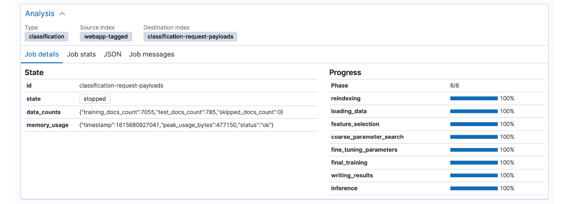
Figure 5.17 – Job analysis pane

The Model evaluation pane displays a confusion matrix. This visualization displays the following:

• True negatives (TNs): Non-malicious events that the model correctly classified as not malicious (represented as false, false)
• True positives (TPs): Malicious events that the model correctly classified as malicious (represented as true, true)
• False positives (FPs): Non-malicious events that the model incorrectly classified as malicious (represented as false, true)
• False negatives (FNs): Malicious events that the model incorrectly classified as not malicious (represented as true, false)

In our example, the model classified all malicious events as malicious and non-malicious events as not malicious, producing the following matrix:

Figure 5.18 – Confusion matrix for the job

The results pane provides fine-grained detail for documents with a prediction and a probability score. Navigate to the Data Frame Analytics page and click on Models to see the trained model.

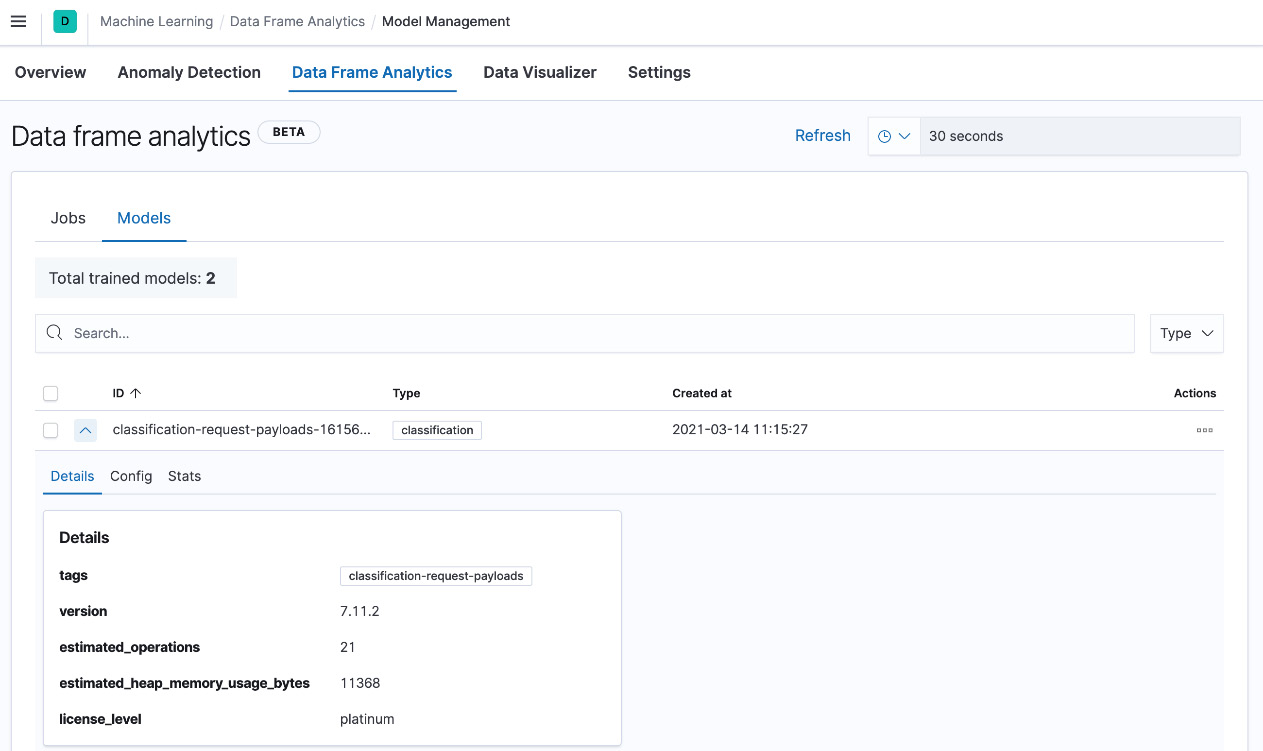
Figure 5.19 – Model details

Now that we have a trained model, the next section will look at using the model to infer classification for new incoming data.

Inferring against incoming data using machine learning

As we learned in Chapter 4, Leveraging Insights and Managing Data on Elasticsearch, ingest pipelines can be used to transform, process, and enrich incoming documents before indexing. Ingest pipelines provide an inference processor to run new documents through a trained machine learning model to infer classification or regression results.

Follow these instructions to create and test an ingest pipeline to run inference using the trained machine learning model:

1. Create a new ingest pipeline as follows. model_id will defer across Kibana instances and can be retrieved from the model pane in the Data Frame Analytics tab on Kibana. model_id in this case is classification-request-payloads-1615680927179:

   PUT _ingest/pipeline/ml-malicious-request

   {

     "processors": [

       {

         "inference": {

           "model_id": "classification-request-payloads-1615680927179",

           "inference_config": {

             "classification": {

               "num_top_classes": 2,

               "results_field": "prediction",

               "top_classes_results_field": "probabilities"

             }

           }

         }

       }

     ]

   }

The inference_config setting can be used to configure the behavior of the inference processor in the ingest pipeline. Detailed configuration settings for the inference processor can be found on the Elasticsearch guide:

https://www.elastic.co/guide/en/elasticsearch/reference/8.0/inference-processor.html.

2. Test the pipeline with sample documents to inspect and confirm inference results. Sample documents are available for testing in Chapter5/ingest-pipelines in the docs-malicious.json and docs-not-malicious.json files.

Pre-prepared simulate requests can be found in the simulate-malicious-docs.json and simulate-not-malicious-docs.json files:

POST _ingest/pipeline/ml-malicious-request/_simulate

{

  "docs": [

    {

      ...

      "_source": {

        "user.name": "u110191",

        "source": {

          "geo": {

            "country_name": "United States",

            ...

          },

          "ip": "64.213.79.243"

        },

        "url": {

          ...

          "full": "https://host-systems.net/user/manage.php"

        },

        "http.request.bytes": "132",

        "event.action": "view",

        "@timestamp": "2021-03-15T10:20:00.000Z",

        "http.request.method": "POST",

        "http.response.bytes": "1417",

        "event.kind": "request",

        "http.response.status_code": "200",

        "event.dataset": "weblogs",

        ...

      }

    }

  ]

}

The API should return output as shown in the following screenshot. The ml object contains inference results, including the predicted label, a prediction score (or confidence), and the probabilities for each class:

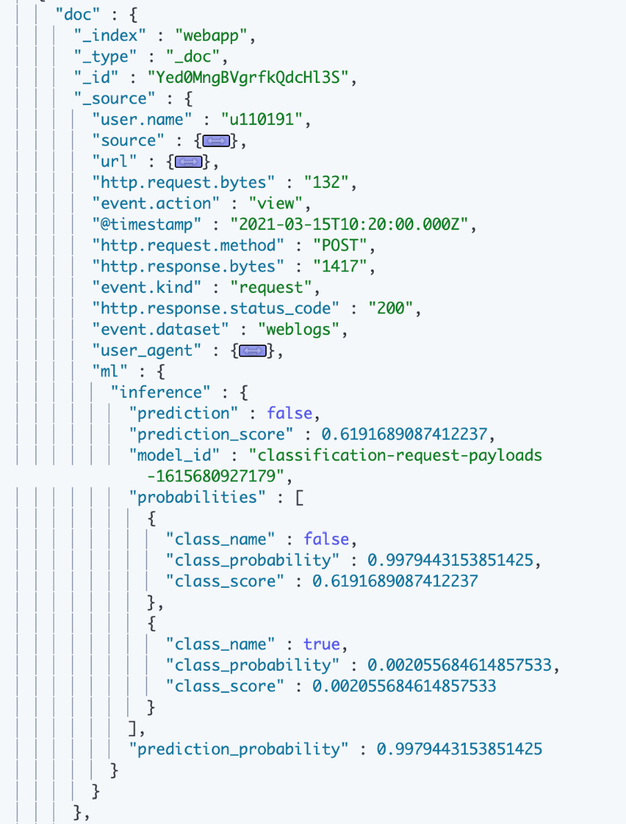
Figure 5.20 – Ingest pipeline results containing inference data

3. As expected, the model correctly classifies the event as not malicious, given the request/response payload sizes are similar in nature to what was seen during normal operation. Use the inference processor to classify documents as they're ingested into Elasticsearch.
4. The ingest pipeline used to transform the incoming data can be updated to include the inference processor. Update the ingest pipeline loaded by the script earlier in the chapter, as follows:

   PUT _ingest/pipeline/webapp-pipeline

   {

     "processors": [

       ...

       {

         "dissect": { ... }

       },

       {

         "remove": { ... }

       },

       {

         "inference": {

           "model_id": "classification-request-payloads-1615680927179",

           "inference_config": {

             "classification": {

               "num_top_classes": 2,

               "results_field": "prediction",

               "top_classes_results_field": "probabilities"

             }

           }

         }

       }

     ]

   }

New documents indexed using the pipeline should now contain inference results from the trained model.

5. Ingest new malicious and benign data, as follows:

   logstash-8.0.0/bin/logstash -f webapp-logstash.conf < webapp-new-data.csv

   logstash-8.0.0/bin/logstash -f webapp-logstash.conf < webapp-password-spraying-attemps.csv

6. Confirm the data contains inference results:

   GET webapp/_search?size=1000

   {

     "query": {

       "exists": {

         "field": "ml"

       }

     }

   }

7. You should see hits containing inference as part of the ml object in the results, as follows:

Figure 5.21 – Indexed documents containing inference results

8. You can now explore the inferred dataset using the Discover tab on Kibana.

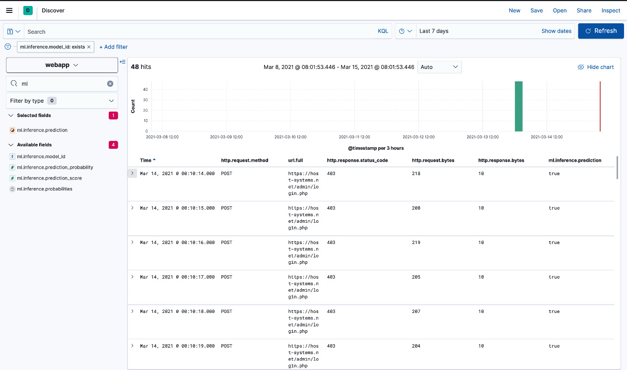
Figure 5.22 – Password spraying attempts with a predicted label

The preceding events indicate password spraying attempts with the machine learning model correctly labeling the events as malicious. Using this information, administrators or analysts can set up alerts or automatic actions (using tools such as Kibana alerting or Watcher) to respond to potential system abuse in the future. We will look at how alerts can be set up to Kibana in Chapter 8, Interacting with Your Data on Kibana.

Summary

In this chapter, we looked at applying supervised and unsupervised machine learning techniques on data in Elasticsearch for various use cases.

First, we explored the use of unsupervised learning to look for anomalous behavior in time series data. We used single-metric, multi-metric, and population jobs to analyze a dataset of web application logs to look for potentially malicious activity.

Next, we looked at the use of supervised learning to train a machine learning model for classifying to classify requests to the web application as malicious using features in the request (primarily the HTTP request/response size values).

Finally, we looked at how the inference processor in ingest pipelines can be used to run continuous inference using a trained model for new data.

In the next chapter, we will move our focus to Beats and their role in the data pipeline. We will look at how different types of events can be collected by Beats agents and sent to Elasticsearch or Logstash for processing.