Relational Databases Lack Relationships

For several decades, developers have tried to accommodate connected, semi-structured datasets inside relational databases. But whereas relational databases were initially designed to codify paper forms and tabular structures—something they do exceedingly well—they struggle when attempting to model the ad hoc, exceptional relationships that crop up in the real world. Ironically, relational databases deal poorly with relationships.

Relationships do exist in the vernacular of relational databases, but only at modeling time, as a means of joining tables. In our discussion of connected data in the previous chapter, we mentioned we often need to disambiguate the semantics of the relationships that connect entities, as well as qualify their weight or strength. Relational relations do nothing of the sort. Worse still, as outlier data multiplies, and the overall structure of the dataset becomes more complex and less uniform, the relational model becomes burdened with large join tables, sparsely populated rows, and lots of null-checking logic. The rise in connectedness translates in the relational world into increased joins, which impede performance and make it difficult for us to evolve an existing database in response to changing business needs.

Figure 2-1 shows a relational schema for storing customer orders in a customer-centric, transactional application.

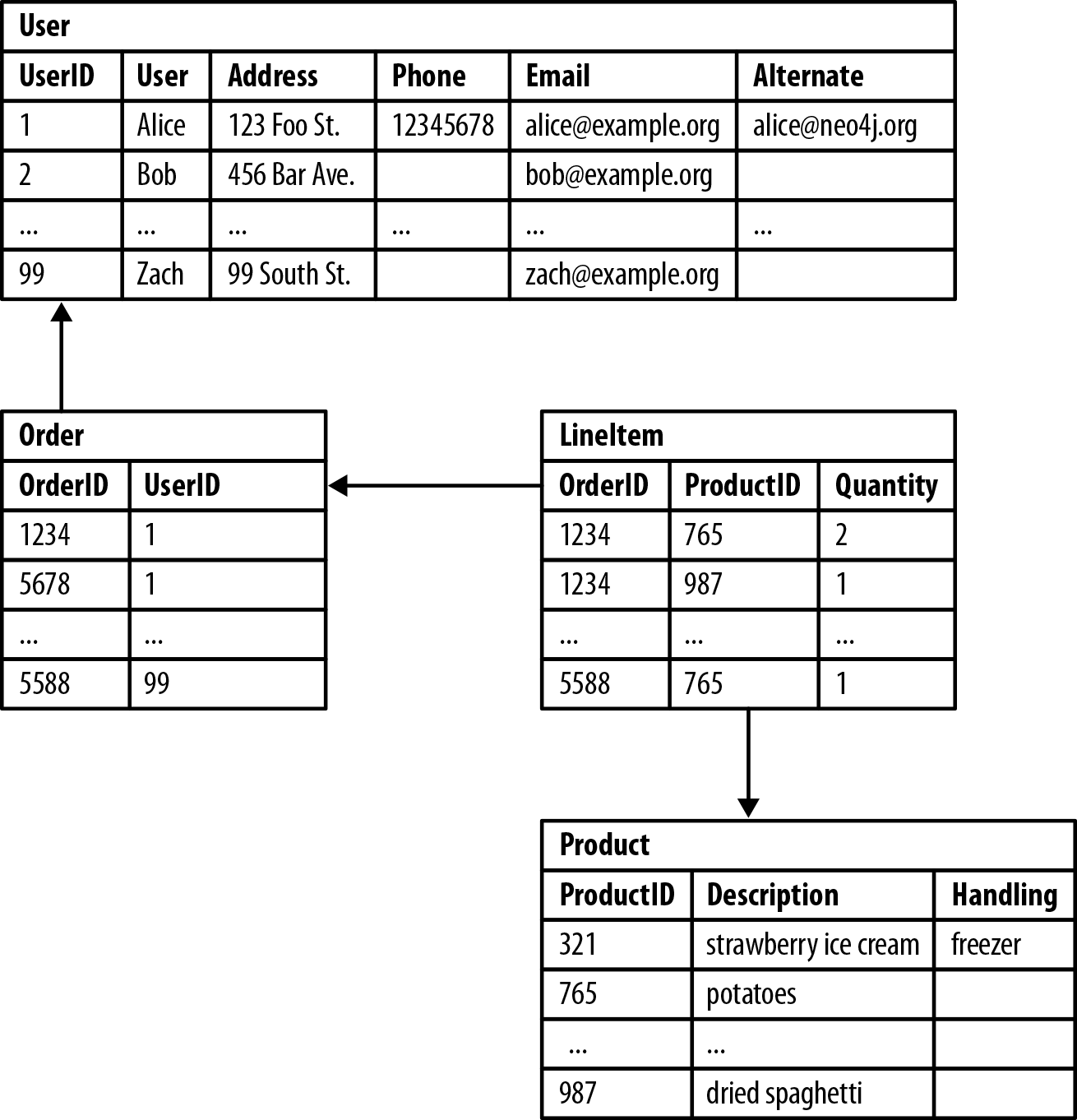
Figure 2-1. Semantic relationships are hidden in a relational database

The application exerts a tremendous influence over the design of this schema, making some queries very easy, and others more difficult:

• Join tables add accidental complexity; they mix business data with foreign key metadata.

• Foreign key constraints add additional development and maintenance overhead just to make the database work.

• Sparse tables with nullable columns require special checking in code, despite the presence of a schema.

• Several expensive joins are needed just to discover what a customer bought.

• Reciprocal queries are even more costly. “What products did a customer buy?” is relatively cheap compared to “which customers bought this product?”, which is the basis of recommendation systems. We could introduce an index, but even with an index, recursive questions such as “which customers buying this product also bought that product?” quickly become prohibitively expensive as the degree of recursion increases.

Relational databases struggle with highly connected domains. To understand the cost of performing connected queries in a relational database, we’ll look at some simple and not-so-simple queries in a social network domain.

Figure 2-2 shows a simple join-table arrangement for recording friendships.

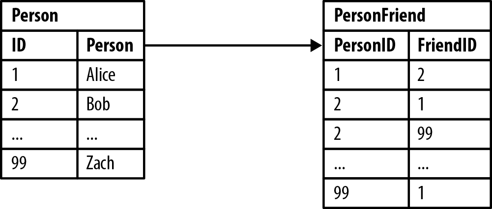
Figure 2-2. Modeling friends and friends-of-friends in a relational database

Asking “who are Bob’s friends?” is easy, as shown in Example 2-1.

SELECT p1.Person
FROM Person p1 JOIN PersonFriend
  ON PersonFriend.FriendID = p1.ID
JOIN Person p2
  ON PersonFriend.PersonID = p2.ID
WHERE p2.Person = 'Bob'

Based on our sample data, the answer is Alice and Zach. This isn’t a particularly expensive or difficult query, because it constrains the number of rows under consideration using the filter WHERE Person.person='Bob'.

Friendship isn’t always a reflexive relationship, so in Example 2-2, we ask the reciprocal query, which is, “who is friends with Bob?”

SELECT p1.Person
FROM Person p1 JOIN PersonFriend
  ON PersonFriend.PersonID = p1.ID
JOIN Person p2
  ON PersonFriend.FriendID = p2.ID
WHERE p2.Person = 'Bob'

The answer to this query is Alice; sadly, Zach doesn’t consider Bob to be a friend. This reciprocal query is still easy to implement, but on the database side it’s more expensive, because the database now has to consider all the rows in the PersonFriend table.

We can add an index, but this still involves an expensive layer of indirection. Things become even more problematic when we ask, “who are the friends of my friends?” Hierarchies in SQL use recursive joins, which make the query syntactically and computationally more complex, as shown in Example 2-3. (Some relational databases provide syntactic sugar for this—for instance, Oracle has a CONNECT BY function—which simplifies the query, but not the underlying computational complexity.)

SELECT p1.Person AS PERSON, p2.Person AS FRIEND_OF_FRIEND
FROM PersonFriend pf1 JOIN Person p1
  ON pf1.PersonID = p1.ID
JOIN PersonFriend pf2
  ON pf2.PersonID = pf1.FriendID
JOIN Person p2
  ON pf2.FriendID = p2.ID
WHERE p1.Person = 'Alice' AND pf2.FriendID <> p1.ID

This query is computationally complex, even though it only deals with the friends of Alice’s friends, and goes no deeper into Alice’s social network. Things get more complex and more expensive the deeper we go into the network. Though it’s possible to get an answer to the question “who are my friends-of-friends-of-friends?” in a reasonable period of time, queries that extend to four, five, or six degrees of friendship deteriorate significantly due to the computational and space complexity of recursively joining tables.

We work against the grain whenever we try to model and query connectedness in a relational database. Besides the query and computational complexity just outlined, we also have to deal with the double-edged sword of schema. More often than not, schema proves to be both too rigid and too brittle. To subvert its rigidity we create sparsely populated tables with many nullable columns, and code to handle the exceptional cases—all because there’s no real one-size-fits-all schema to accommodate the variety in the data we encounter. This increases coupling and all but destroys any semblance of cohesion. Its brittleness manifests itself as the extra effort and care required to migrate from one schema to another as an application evolves.

NOSQL Databases Also Lack Relationships

Most NOSQL databases—whether key-value-, document-, or column-oriented—store sets of disconnected documents/values/columns. This makes it difficult to use them for connected data and graphs.

One well-known strategy for adding relationships to such stores is to embed an aggregate’s identifier inside the field belonging to another aggregate—effectively introducing foreign keys. But this requires joining aggregates at the application level, which quickly becomes prohibitively expensive.

When we look at an aggregate store model, such as the one in Figure 2-3, we imagine we can see relationships. Seeing a reference to order: 1234 in the record beginning user: Alice, we infer a connection between user: Alice and order: 1234. This gives us false hope that we can use keys and values to manage graphs.

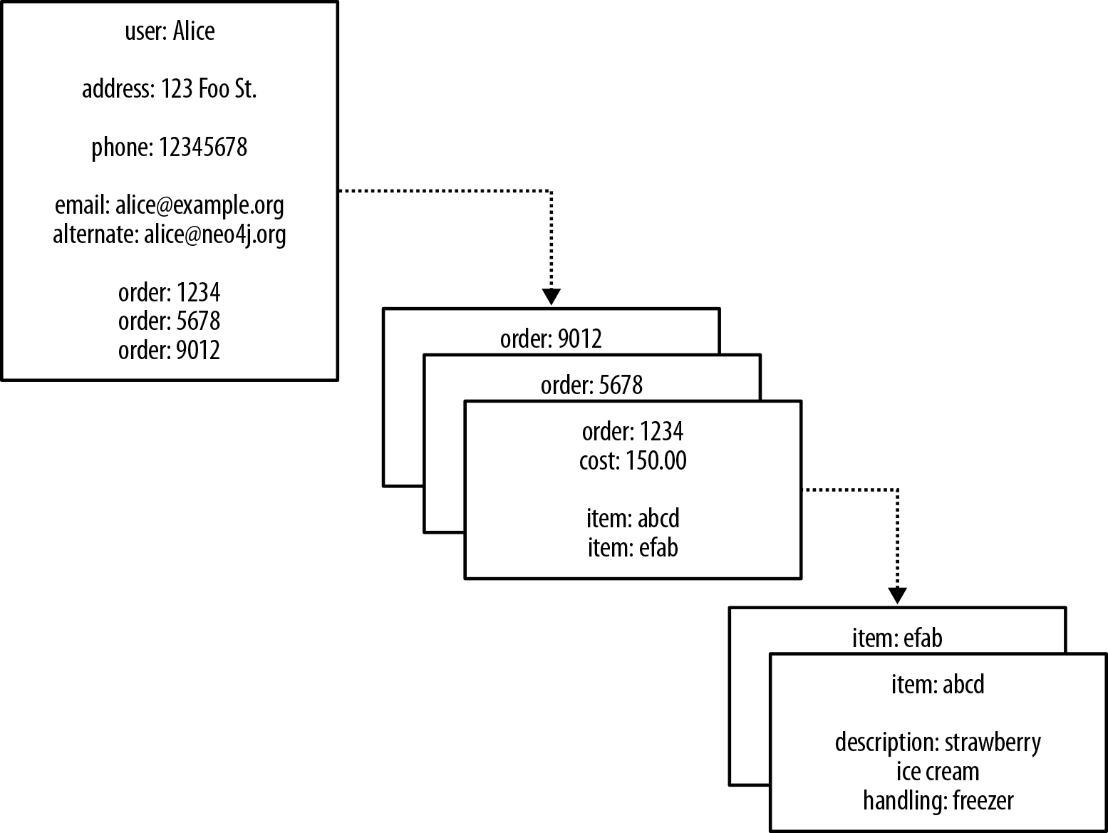
Figure 2-3. Reifying relationships in an aggregate store

In Figure 2-3 we infer that some property values are really references to foreign aggregates elsewhere in the database. But turning these inferences into a navigable structure doesn’t come for free, because relationships between aggregates aren’t first-class citizens in the data model—most aggregate stores furnish only the insides of aggregates with structure, in the form of nested maps. Instead, the application that uses the database must build relationships from these flat, disconnected data structures. We also have to ensure that the application updates or deletes these foreign aggregate references in tandem with the rest of the data. If this doesn’t happen, the store will accumulate dangling references, which can harm data quality and query performance.

There’s another weak point in this scheme. Because there are no identifiers that “point” backward (the foreign aggregate “links” are not reflexive, of course), we lose the ability to run other interesting queries on the database. For example, with the structure shown in Figure 2-3, asking the database who has bought a particular product—perhaps for the purpose of making a recommendation based on a customer profile—is an expensive operation. If we want to answer this kind of question, we will likely end up exporting the dataset and processing it via some external compute infrastructure, such as Hadoop, to brute-force compute the result. Alternatively, we can retrospectively insert backward-pointing foreign aggregate references, and then query for the result. Either way, the results will be latent.

It’s tempting to think that aggregate stores are functionally equivalent to graph databases with respect to connected data. But this is not the case. Aggregate stores do not maintain consistency of connected data, nor do they support what is known as index-free adjacency, whereby elements contain direct links to their neighbors. As a result, for connected data problems, aggregate stores must employ inherently latent methods for creating and querying relationships outside the data model.

Let’s see how some of these limitations manifest themselves. Figure 2-4 shows a small social network as implemented using documents in an aggregate store.

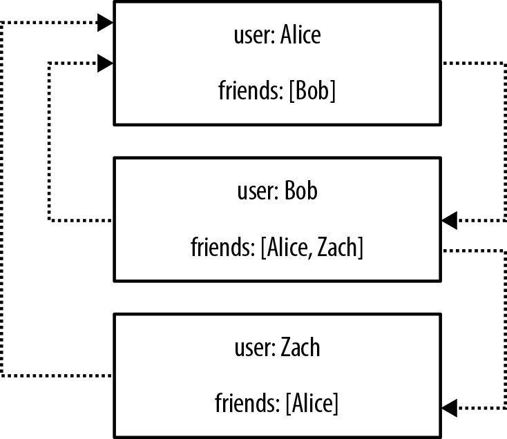
Figure 2-4. A small social network encoded in an aggregate store

With this structure, it’s easy to find a user’s immediate friends—assuming, of course, the application has been diligent in ensuring identifiers stored in the friends property are consistent with other record IDs in the database. In this case we simply look up immediate friends by their ID, which requires numerous index lookups (one for each friend) but no brute-force scans of the entire dataset. Doing this, we’d find, for example, that Bob considers Alice and Zach to be friends.

But friendship isn’t always symmetric. What if we’d like to ask “who is friends with Bob?” rather than “who are Bob’s friends?” That’s a more difficult question to answer, and in this case our only option would be to brute-force scan across the whole dataset looking for friends entries that contain Bob.

To avoid having to process the entire dataset, we could denormalize the storage model by adding backward links. Adding a second property, called perhaps friended_by, to each user, we can list the incoming friendship relations associated with that user. But this doesn’t come for free. For starters, we have to pay the initial and ongoing cost of increased write latency, plus the increased disk utilization cost for storing the additional metadata. On top of that, traversing the links remains expensive, because each hop requires an index lookup. This is because aggregates have no notion of locality, unlike graph databases, which naturally provide index-free adjacency through real—not reified—relationships. By implementing a graph structure atop a nonnative store, we get some of the benefits of partial connectedness, but at substantial cost.

This substantial cost is amplified when it comes to traversing deeper than just one hop. Friends are easy enough, but imagine trying to compute—in real time—friends-of-friends, or friends-of-friends-of-friends. That’s impractical with this kind of database because traversing a fake relationship isn’t cheap. This not only limits your chances of expanding your social network, it also reduces profitable recommendations, misses faulty equipment in your data center, and lets fraudulent purchasing activity slip through the net. Many systems try to maintain the appearance of graph-like processing, but inevitably it’s done in batches and doesn’t provide the real-time interaction that users demand.

Graph Databases Embrace Relationships

The previous examples have dealt with implicitly connected data. As users we infer semantic dependencies between entities, but the data models—and the databases themselves—are blind to these connections. To compensate, our applications must create a network out of the flat, disconnected data at hand, and then deal with any slow queries and latent writes across denormalized stores that arise.

What we really want is a cohesive picture of the whole, including the connections between elements. In contrast to the stores we’ve just looked at, in the graph world, connected data is stored as connected data. Where there are connections in the domain, there are connections in the data. For example, consider the social network shown in Figure 2-5.

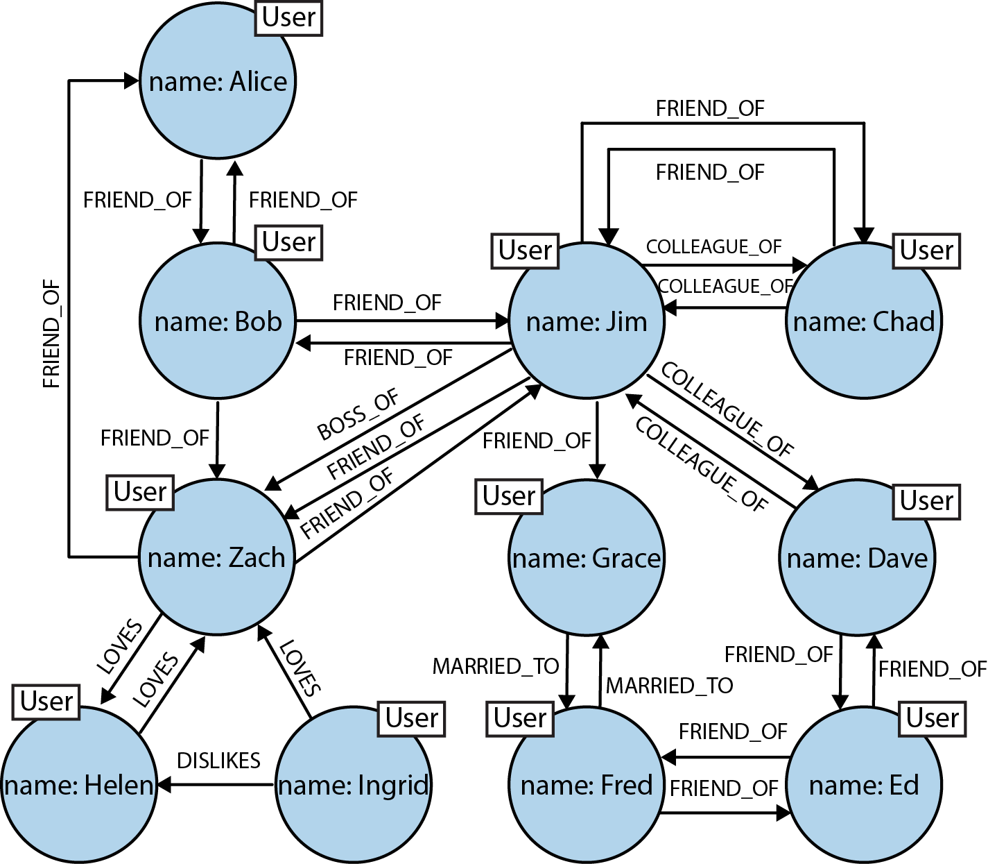
Figure 2-5. Easily modeling friends, colleagues, workers, and (unrequited) lovers in a graph

In this social network, as in so many real-world cases of connected data, the connections between entities don’t exhibit uniformity across the domain—the domain is variably-structured. A social network is a popular example of a densely connected, variably-structured network, one that resists being captured by a one-size-fits-all schema or conveniently split across disconnected aggregates. Our simple network of friends has grown in size (there are now potential friends up to six degrees away) and expressive richness. The flexibility of the graph model has allowed us to add new nodes and new relationships without compromising the existing network or migrating data—the original data and its intent remain intact.

The graph offers a much richer picture of the network. We can see who LOVES whom (and whether that love is requited). We can see who is a COLLEAGUE_OF whom, and who is BOSS_OF them all. We can see who’s off the market, because they’re MARRIED_TO someone else; we can even see the antisocial elements in our otherwise social network, as represented by DISLIKES relationships. With this graph at our disposal, we can now look at the performance advantages of graph databases when dealing with connected data.

Relationships in a graph naturally form paths. Querying—or traversing—the graph involves following paths. Because of the fundamentally path-oriented nature of the data model, the majority of path-based graph database operations are highly aligned with the way in which the data is laid out, making them extremely efficient. In their book Neo4j in Action, Partner and Vukotic perform an experiment using both a relational store and Neo4j. The comparison shows that the graph database (in this case, Neo4j and its Traversal Framework) is substantially quicker for connected data than a relational store.

Partner and Vukotic’s experiment seeks to find friends-of-friends in a social network, to a maximum depth of five. For a social network containing 1,000,000 people, each with approximately 50 friends, the results strongly suggest that graph databases are the best choice for connected data, as we see in Table 2-1.

At depth two (friends-of-friends), both the relational database and the graph database perform well enough for us to consider using them in an online system. Although the Neo4j query runs in two-thirds the time of the relational one, an end user would barely notice the difference in milliseconds between the two. By the time we reach depth three (friend-of-friend-of-friend), however, it’s clear that the relational database can no longer deal with the query in a reasonable time frame: the 30 seconds it takes to complete would be completely unacceptable for an online system. In contrast, Neo4j’s response time remains relatively flat: just a fraction of a second to perform the query—definitely quick enough for an online system.

At depth four the relational database exhibits crippling latency, making it practically useless for an online system. Neo4j’s timings have deteriorated a little too, but the latency here is at the periphery of being acceptable for a responsive online system. Finally, at depth five, the relational database simply takes too long to complete the query. Neo4j, in contrast, returns a result in around two seconds. At depth five, it turns out that almost the entire network is our friend. Because of this, for many real-world use cases we’d likely trim the results, thereby reducing the timings.

The social network example helps illustrate how different technologies deal with connected data, but is it a valid use case? Do we really need to find such remote “friends”? Perhaps not. But substitute any other domain for the social network, and you’ll see we experience similar performance, modeling, and maintenance benefits. Whether music or data center management, bio-informatics or football statistics, network sensors or time-series of trades, graphs provide powerful insight into our data. Let’s look, then, at another contemporary application of graphs: recommending products based on a user’s purchase history and the histories of his friends, neighbors, and other people like him. With this example, we’ll bring together several independent facets of a user’s lifestyle to make accurate and profitable recommendations.

We’ll start by modeling the purchase history of a user as connected data. In a graph, this is as simple as linking the user to her orders, and linking orders together to provide a purchase history, as shown in Figure 2-6.

The graph shown in Figure 2-6 provides a great deal of insight into customer behavior. We can see all the orders a user has PLACED, and we can easily reason about what each order CONTAINS. To this core domain data structure we’ve then added support for several well-known access patterns. For example, users often want to see their order history, so we’ve added a linked list structure to the graph that allows us to find a user’s most recent order by following an outgoing MOST_RECENT relationship. We can then iterate through the list, going further back in time, by following each PREVIOUS relationship. If we want to move forward in time, we can follow each PREVIOUS relationship in the opposite direction, or add a reciprocal NEXT relationship.

Now we can start to make recommendations. If we notice that many users who buy strawberry ice cream also buy espresso beans, we can start to recommend those beans to users who normally only buy the ice cream. But this is a rather one-dimensional recommendation: we can do much better. To increase our graph’s power, we can join it to graphs from other domains. Because graphs are naturally multidimensional structures, it’s then quite straightforward to ask more sophisticated questions of the data to gain access to a fine-tuned market segment. For example, we can ask the graph to find for us “all the flavors of ice cream liked by people who enjoy espresso but dislike Brussels sprouts, and who live in a particular neighborhood.”

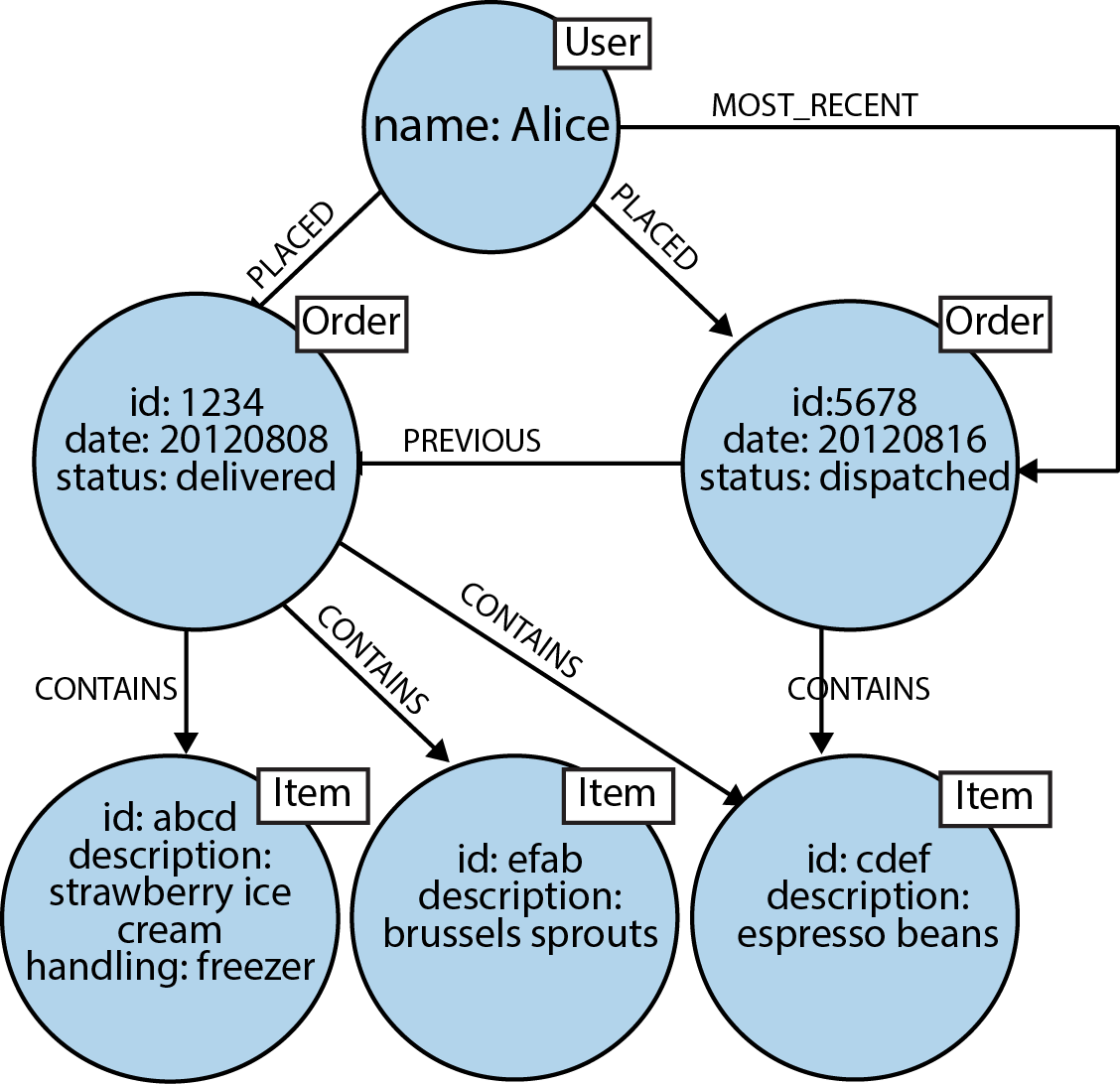
Figure 2-6. Modeling a user’s order history in a graph

For the purpose of our interpretation of the data, we can consider the degree to which someone repeatedly buys a product to be indicative of whether or not they like that product. But how might we define “live in a neighborhood”? Well, it turns out that geospatial coordinates are very conveniently modeled as graphs. One of the most popular structures for representing geospatial coordinates is called an R-Tree. An R-Tree is a graph-like index that describes bounded boxes around geographies. Using such a structure we can describe overlapping hierarchies of locations. For example, we can represent the fact that London is in the UK, and that the postal code SW11 1BD is in Battersea, which is a district in London, which is in southeastern England, which, in turn, is in Great Britain. And because UK postal codes are fine-grained, we can use that boundary to target people with somewhat similar tastes.¹

We can use our example graph to make recommendations to users, but we can also use it to benefit the seller. For example, given certain buying patterns (products, cost of typical order, and so on), we can establish whether a particular transaction is potentially fraudulent. Patterns outside of the norm for a given user can easily be detected in a graph and then flagged for further attention (using well-known similarity measures from the graph data-mining literature), thus reducing the risk for the seller.²

From the data practitioner’s point of view, it’s clear that the graph database is the best technology for dealing with complex, variably structured, densely connected data—that is, with datasets so sophisticated they are unwieldy when treated in any form other than a graph.

Summary

In this chapter we’ve seen how connectedness in relational databases and NOSQL data stores requires developers to implement data processing in the application layer, and contrasted that with graph databases, where connectedness is a first-class citizen. In the next chapter, we look in more detail at the topic of graph modeling.