The Rise of NOSQL

Historically, most enterprise-level web apps ran on top of a relational database. But in the past decade, we’ve been faced with data that is bigger in volume, changes more rapidly, and is more structurally varied than can be dealt with by traditional RDBMS deployments. The NOSQL movement has arisen in response to these challenges.

It’s no surprise that as storage has increased dramatically, volume has become the principal driver behind the adoption of NOSQL stores by organizations. Volume may be defined simply as the size of the stored data.

As is well known, large datasets become unwieldy when stored in relational databases. In particular, query execution times increase as the size of tables and the number of joins grow (so-called join pain). This isn’t the fault of the databases themselves. Rather, it is an aspect of the underlying data model, which builds a set of all possible answers to a query before filtering to arrive at the correct solution.

In an effort to avoid joins and join pain, and thereby cope better with extremely large datasets, the NOSQL world has adopted several alternatives to the relational model. Though more adept at dealing with very large datasets, these alternative models tend to be less expressive than the relational one (with the exception of the graph model, which is actually more expressive).

But volume isn’t the only problem modern web-facing systems have to deal with. Besides being big, today’s data often changes very rapidly. Velocity is the rate at which data changes over time.

Velocity is rarely a static metric. Internal and external changes to a system and the context in which it is employed can have considerable impact on velocity. Coupled with high volume, variable velocity requires data stores to not only handle sustained levels of high write loads, but also deal with peaks.

There is another aspect to velocity, which is the rate at which the structure of the data changes. In other words, in addition to the value of specific properties changing, the overall structure of the elements hosting those properties can change as well. This commonly occurs for two reasons. The first is fast-moving business dynamics. As the business changes, so do its data needs. The second is that data acquisition is often an experimental affair. Some properties are captured “just in case,” others are introduced at a later point based on changed needs. The ones that prove valuable to the business stay around, others fall by the wayside. Both these forms of velocity are problematic in the relational world, where high write loads translate into a high processing cost, and high schema volatility has a high operational cost.

Although commentators have later added other useful requirements to the original quest for scale, the final key aspect is the realization that data is far more varied than the data we’ve dealt with in the relational world. For existential proof, think of all those nulls in our tables and the null checks in our code. This has driven out the final widely agreed upon facet, variety, which we define as the degree to which data is regularly or irregularly structured, dense or sparse, connected or disconnected.

ACID versus BASE

When we first encounter NOSQL it’s often in the context of what many of us are already familiar with: relational databases. Although we know the data and query model will be different (after all, there’s no SQL), the consistency models used by NOSQL stores can also be quite different from those employed by relational databases. Many NOSQL databases use different consistency models to support the differences in volume, velocity, and variety of data discussed earlier.

Let’s explore what consistency features are available to help keep data safe, and what trade-offs are involved when using (most) NOSQL stores.¹

In the relational database world, we’re all familiar with ACID transactions, which have been the norm for some time. The ACID guarantees provide us with a safe environment in which to operate on data:

Atomic

All operations in a transaction succeed or every operation is rolled back.

Consistent

On transaction completion, the database is structurally sound.

Isolated

Transactions do not contend with one another. Contentious access to state is moderated by the database so that transactions appear to run sequentially.

Durable

The results of applying a transaction are permanent, even in the presence of failures.

These properties mean that once a transaction completes, its data is consistent (so-called write consistency) and stable on disk (or disks, or indeed in multiple distinct memory locations). This is a wonderful abstraction for the application developer, but requires sophisticated locking, which can cause logical unavailability, and is typically considered to be a heavyweight pattern for most use cases.

For many domains, ACID transactions are far more pessimistic than the domain actually requires. In the NOSQL world, ACID transactions have gone out of fashion as stores loosen the requirements for immediate consistency, data freshness, and accuracy in order to gain other benefits, like scale and resilience. Instead of using ACID, the term BASE has arisen as a popular way of describing the properties of a more optimistic storage strategy:

Basic availability

The store appears to work most of the time.

Soft-state

Stores don’t have to be write-consistent, nor do different replicas have to be mutually consistent all the time.

Eventual consistency

Stores exhibit consistency at some later point (e.g., lazily at read time).

The BASE properties are considerably looser than the ACID guarantees, and there is no direct mapping between them. A BASE store values availability (because that is a core building block for scale), but does not offer guaranteed consistency of replicas at write time. BASE stores provide a less strict assurance: that data will be consistent in the future, perhaps at read time (e.g., Riak), or will always be consistent, but only for certain processed past snapshots (e.g., Datomic).

Given such loose support for consistency, we as developers need to be more knowledgable and rigorous when considering data consistency. We must be familiar with the BASE behavior of our chosen stores and work within those constraints. At the application level we must choose on a case-by-case basis whether we will accept potentially inconsistent data, or whether we will instruct the database to provide consistent data at read time, while incurring the latency penalty that that implies. (In order to guarantee consistent reads, the database will need to compare all replicas of a data element, and in an inconsistent outcome even perform remedial repair work on that data.) From a development perspective this is a far cry from the simplicity of relying on transactions to manage consistent state on our behalf, and though that’s not necessarily a bad thing, it does require effort.

The NOSQL Quadrants

Having discussed the BASE model that underpins consistency in NOSQL stores, we’re ready to start looking at the numerous user-level data models. To disambiguate these models, we’ve devised a simple taxonomy, as shown in Figure A-1. This taxonomy divides the contemporary NOSQL space into four quadrants. Stores in each quadrant address a different kind of functional use case—though nonfunctional requirements can also strongly influence our choice of database.

In the following sections we’ll deal with each of these quadrants, highlighting the characteristics of the data model, operational aspects, and drivers for adoption.

Document Stores

Document databases offer the most immediately familiar paradigm for developers used to working with hierarchically structured documents. Document databases store and retrieve documents, just like an electronic filing cabinet. Documents tend to comprise maps and lists, allowing for natural hierarchies—much as we’re used to with formats like JSON and XML.

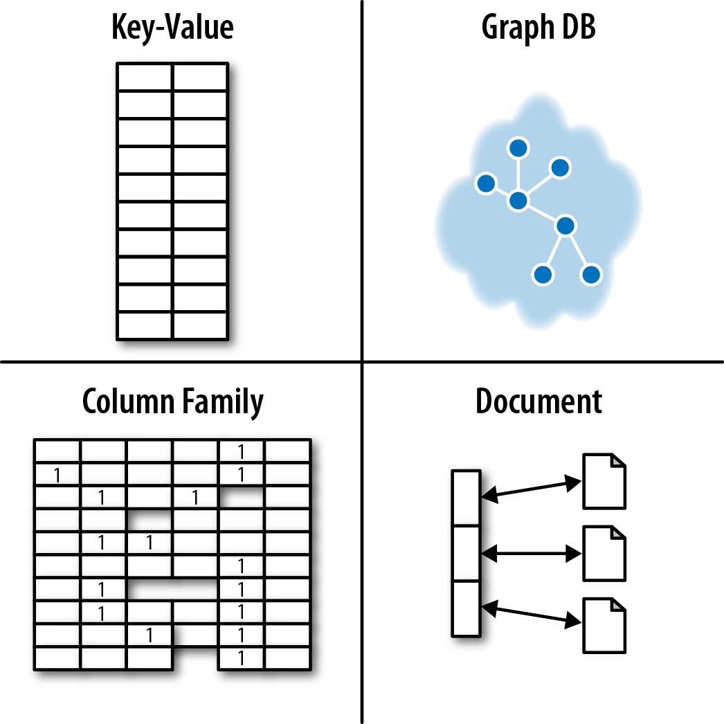
Figure A-1. The NOSQL store quadrants

At the simplest level, documents can be stored and retrieved by ID. Providing an application remembers the IDs it’s interested in (e.g., usernames), a document store can act much like a key-value store (of which we’ll see more later). But in the general case, document stores rely on indexes to facilitate access to documents based on their attributes. For example, in an ecommerce scenario, we might use indexes to represent distinct product types so that they can be offered up to potential sellers, as shown in Figure A-2. In general, indexes are used to retrieve sets of related documents from the store for an application to use.

Much like indexes in relational databases, indexes in a document store enable us to trade write performance for greater read performance. Writes are more costly, because they also maintain indexes, but reads require scanning fewer records to find pertinent data. For write-heavy records, it’s worth bearing in mind that indexes might actually degrade performance overall.

Where data hasn’t been indexed, queries are typically much slower, because a full search of the dataset has to happen. This is obviously an expensive task and is to be avoided wherever possible—and as we shall see, rather than process these queries internally, it’s normal for document database users to externalize this kind of processing in parallel compute frameworks.

Figure A-2. Indexing reifies sets of entities in a document store

Because the data model of a document store is one of disconnected entities, document stores tend to have interesting and useful operational characteristics. They should scale horizontally, due to there being no contended state between mutually independent records at write time, and no need to transact across replicas.

For writes, document databases have, historically, provided transactionality limited to the level of an individual record. That is, a document database will ensure that writes to a single document are atomic—assuming the administrator has opted for safe levels of persistence when setting up the database. Support for operating across sets of documents atomically is emerging in this category, but it is not yet mature. In the absence of multikey transactions, it is down to application developers to write compensating logic in application code.

Because stored documents are not connected (except through indexes), there are numerous optimistic concurrency control mechanisms that can be used to help reconcile concurrent contending writes for a single document without having to resort to strict locks. In fact, some document stores (like CouchDB) have made this a key point of their value proposition: documents can be held in a multimaster database that automatically replicates concurrently accessed, contended state across instances without undue interference from the user.

In other stores, the database management system may also be able to distinguish and reconcile writes to different parts of a document, or even use timestamps to reconcile several contended writes into a single logically consistent outcome. This is a reasonable optimistic trade-off insofar as it reduces some of the need for transactions by using alternative mechanisms that optimistically control storage while striving to provide lower latency and higher throughput.

Key-Value Stores

Key-value stores are cousins of the document store family, but their lineage comes from Amazon’s Dynamo database. They act like large, distributed hashmap data structures that store and retrieve opaque values by key.

As shown in Figure A-3, the key space of the hashmap is spread across numerous buckets on the network. For fault-tolerance reasons, each bucket is replicated onto several machines. The formula for number of replicas required is given by R = 2F +1, where F is the number of failures we can tolerate. The replication algorithm seeks to ensure that machines aren’t exact copies of each other. This allows the system to load-balance while a machine and its buckets recover. It also helps avoid hotspots, which can cause inadvertent self denial-of-service.

From the client’s point of view, key-value stores are easy to use. A client stores a data element by hashing a domain-specific identifier (key). The hash function is crafted such that it provides a uniform distribution across the available buckets, thereby ensuring that no single machine becomes a hotspot. Given the hashed key, the client can use that address to store the value in a corresponding bucket. Clients use a similar process to retrieve stored values.

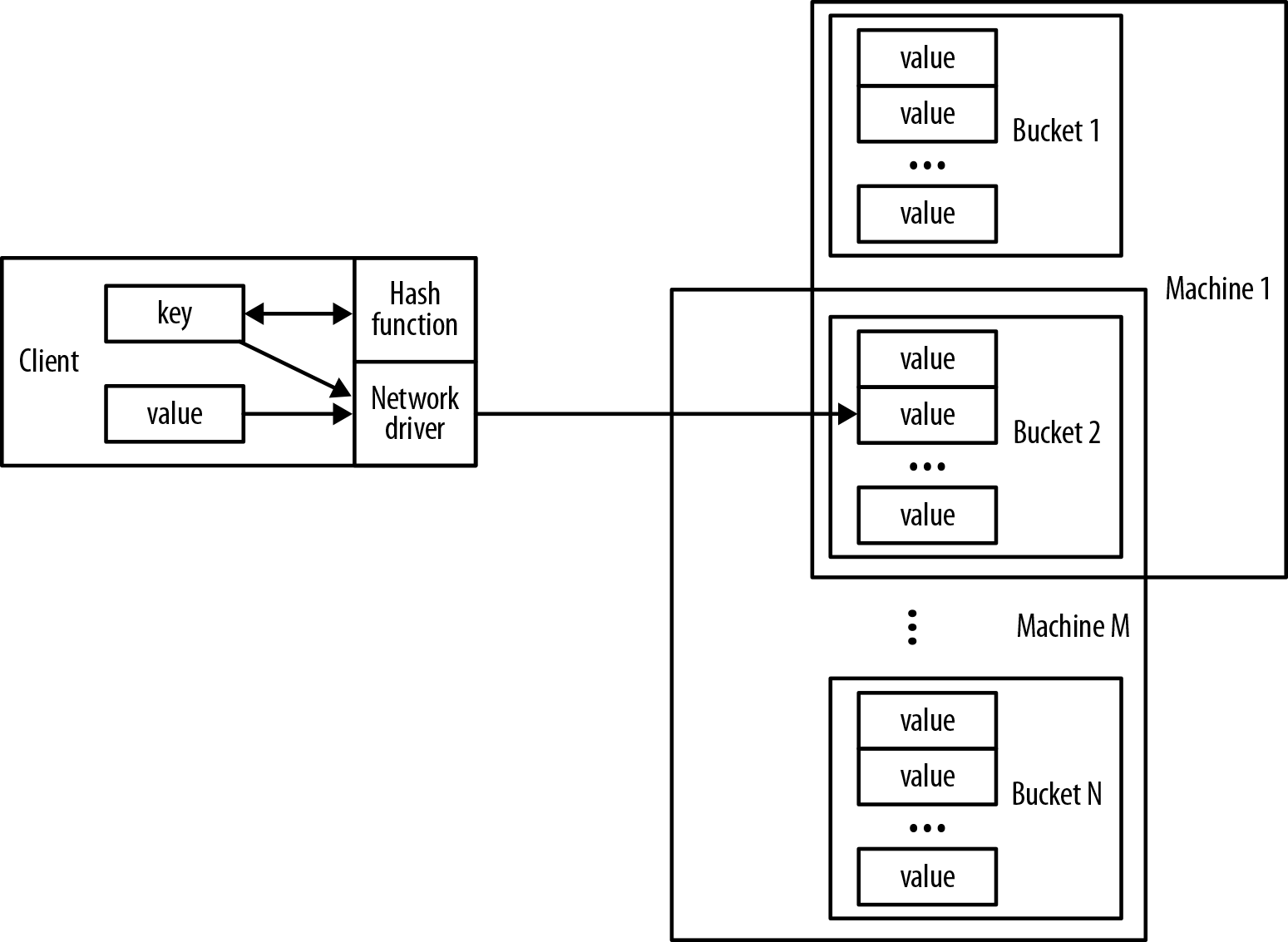
Figure A-3. Key-value stores act like distributed hashmap data structures

Given such a model, applications wishing to store data in, or retrieve data from, a key-value store need only know (or compute) the corresponding key. Although there is a very large number of possible keys in the key set, in practice keys tend to fall out quite naturally from the application domain. Usernames and email addresses, Cartesian coordinates for places of interest, Social Security numbers, and zip codes are all natural keys for various domains. With a sensibly designed system, the chance of losing data in the store due to a missing key is low.

The key-value data model is similar to the document data model. What differentiates them is the level of insight each offers into its data.

In theory, key-value stores are oblivious to the information contained in their values. Pure key-value stores simply concern themselves with efficient storage and retrieval of opaque data on behalf of applications, unencumbered by its nature and application usage.

In practice, such distinctions aren’t always so clear-cut. Some of the popular key-value stores—Riak, for instance—also offer visibility into certain types of structured stored data like XML and JSON. It also supports some core data types (called CRDTs) that can be confidently merged even in the presence of concurrent writes. At a product level, then, there is some overlap between the document and key-value stores.

Although simple, the key-value model, much as the document model, offers little in the way of data insight to the application developer. To retrieve sets of useful information from across individual records, we typically use an external processing infrastructure, such as MapReduce. This is highly latent compared to executing queries in the data store.

Key-value stores offer certain operational and scale advantages. Descended as they are from Amazon’s Dynamo database—a platform designed for a nonstop shopping cart service—they tend to be optimized for high availability and scale. Or, as the Amazon team puts it, they should work even “if disks are failing, network routes are flapping, or data centers are being destroyed by tornados.”

Column Family

Column family stores are modeled on Google’s BigTable. The data model is based on a sparsely populated table whose rows can contain arbitrary columns, the keys for which provide natural indexing.

In Figure A-4, we see the four common building blocks used in column family databases. The simplest unit of storage is the column itself, consisting of a name-value pair. Any number of columns can be combined into a super column, which gives a name to a sorted set of columns. Columns are stored in rows, and when a row contains columns only, it is known as a column family. When a row contains super columns, it is known as a super column family.

Figure A-4. The four building blocks of column family storage

It might seem odd to focus on rows when the data model is ostensibly columnar, but individual rows are important, because they provide the nested hashmap structure into which we denormalize our data. In Figure A-5 we show how we might map a recording artist and his albums into a super column family structure—logically, it’s really nothing more than maps of maps.

Figure A-5. Storing line-of-business data in a super column family

In a column family database, each row in the table represents a particular overarching entity (e.g., everything about an artist). These column families are containers for related pieces of data, such as the artist’s name and discography. Within the column families we find actual key-value data, such as album release dates and the artist’s date of birth.

Helpfully, this row-oriented view can be turned 90 degrees to arrive at a column-oriented view. Where each row gives a complete view of one entity, the column view naturally indexes particular aspects across the whole dataset. For example, as we see in Figure A-6, by “lining up” keys we are able to find all the rows where the artist is English. From there it’s easy to extract complete artist data from each row. It’s not connected data as we’d find in a graph, but it does at least provide some insight into a set of related entities.

Column family databases are distinguished from document and key-value stores not only by their more expressive data model, but also by their operational characteristics. Apache Cassandra, for example, which is based on a Dynamo-like infrastructure, is architected for distribution, scale, and failover. Under the covers it uses several storage engines that deal with high write loads—the kind of peak write loads generated by popular interactive TV shows.

Figure A-6. Keys form a natural index through rows in a column family database

Overall, column family databases are reasonably expressive, and operationally very competent. And yet they’re still aggregate stores, just like document and key-value databases, and as such still lack joins. Querying them for insight into data at scale requires processing by some external application infrastructure.

Query versus Processing in Aggregate Stores

In the preceding sections we’ve highlighted the similarities and differences between the document, key-value, and column family data models. On balance, the similarities are greater than the differences. In fact, the similarities are so great, the three types are sometimes referred to jointly as aggregate stores. Aggregate stores persist standalone complex records that reflect the Domain-Driven Design notion of an aggregate.

Though each aggregate store has a different storage strategy, they all have a great deal in common when it comes to querying data. For simple ad hoc queries, each tends to provide features such as indexing, simple document linking, or a query language. For more complex queries, applications commonly identify and extract a subset of data from the store before piping it through some external processing infrastructure such as a MapReduce framework. This is done when the necessary deep insight cannot be generated simply by examining individual aggregates.

MapReduce, like BigTable, is another technique that comes to us from Google. The most prevalent open source implementation of MapReduce is Apache Hadoop and its attendant ecosystem.

MapReduce is a parallel programming model that splits data and operates on it in parallel before gathering it back together and aggregating it to provide focused information. If, for example, we wanted to use it to count how many American artists there are in a recording artists database, we’d extract all the artist records and discard the non-American ones in the map phase, and then count the remaining records in the reduce phase.

Even with a lot of machines and a fast network infrastructure, MapReduce can be quite latent. Normally, we’d use the features of the data store to provide a more focused dataset—perhaps using indexes or other ad hoc queries—and then MapReduce that smaller dataset to arrive at our answer.

Aggregate stores are not built to deal with highly connected data. We can try to use them for that purpose, but we have to add code to fill in where the underlying data model leaves off, resulting in a development experience that is far from seamless, and operational characteristics that are generally speaking not very fast, particularly as the number of hops (or “degree” of the query) increases. Aggregate stores may be good at storing data that’s big, but they aren’t great at dealing with problems that require an understanding of how things are connected.

Graph Databases

A graph database is an online, operational database management system with Create, Read, Update, and Delete (CRUD) methods that expose a graph data model. Graph databases are generally built for use with transactional (OLTP) systems. Accordingly, they are normally optimized for transactional performance, and engineered with transactional integrity and operational availability in mind.

Two properties of graph databases are useful to understand when investigating graph database technologies:

The underlying storage

Some graph databases use native graph storage, which is optimized and designed for storing and managing graphs. Not all graph database technologies use native graph storage, however. Some serialize the graph data into a relational database, object-oriented database, or other types of NOSQL stores.

The processing engine

Some definitions of graph databases require that they be capable of index-free adjacency, meaning that connected nodes physically “point” to each other in the database.² Here we take a slightly broader view. Any database that from the user’s perspective behaves like a graph database (i.e., exposes a graph data model through CRUD operations), qualifies as a graph database. We do acknowledge, however, the significant performance advantages of index-free adjacency, and therefore use the term native graph processing in reference to graph databases that leverage index-free adjacency.

Graph databases—in particular native ones—don’t depend heavily on indexes because the graph itself provides a natural adjacency index. In a native graph database, the relationships attached to a node naturally provide a direct connection to other related nodes of interest. Graph queries use this locality to traverse through the graph by chasing pointers. These operations can be carried out with extreme efficiency, traversing millions of nodes per second, in contrast to joining data through a global index, which is many orders of magnitude slower.

Besides adopting a specific approach to storage and processing, a graph database will also adopt a specific data model. There are several different graph data models in common usage, including property graphs, hypergraphs, and triples. We discuss each of these models below.

Hypergraphs

A hypergraph is a generalized graph model in which a relationship (called a hyper-edge) can connect any number of nodes. Whereas the property graph model permits a relationship to have only one start node and one end node, the hypergraph model allows any number of nodes at either end of a relationship. Hypergraphs can be useful where the domain consists mainly of many-to-many relationships. For example, in Figure A-7 we see that Alice and Bob are the owners of three vehicles. We express this using a single hyper-edge, whereas in a property graph we would use six relationships.

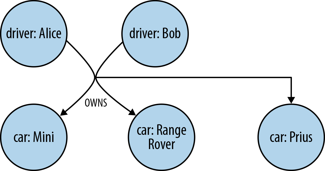
Figure A-7. A simple (directed) hypergraph

As we discussed in Chapter 3, graphs enable us to model our problem domain in a way that is easy to visualize and understand, and which captures with high fidelity the many nuances of the data we encounter in the real world. Although in theory hypergraphs produce accurate, information-rich models, in practice it’s very easy for us to miss some detail while modeling. To illustrate this point, let’s consider the graph shown in Figure A-8, which is the property graph equivalent of the hypergraph shown in Figure A-7.

The property graph shown here requires several OWNS relationships to express what the hypergraph captured with just one. But in using several relationships, not only are we able to use a familiar and very explicit modeling technique, but we’re also able to fine-tune the model. For example, we’ve identified the “primary driver” for each vehicle (for insurance purposes) by adding a property to the relevant relationships—something that can’t be done with a single hyper-edge.

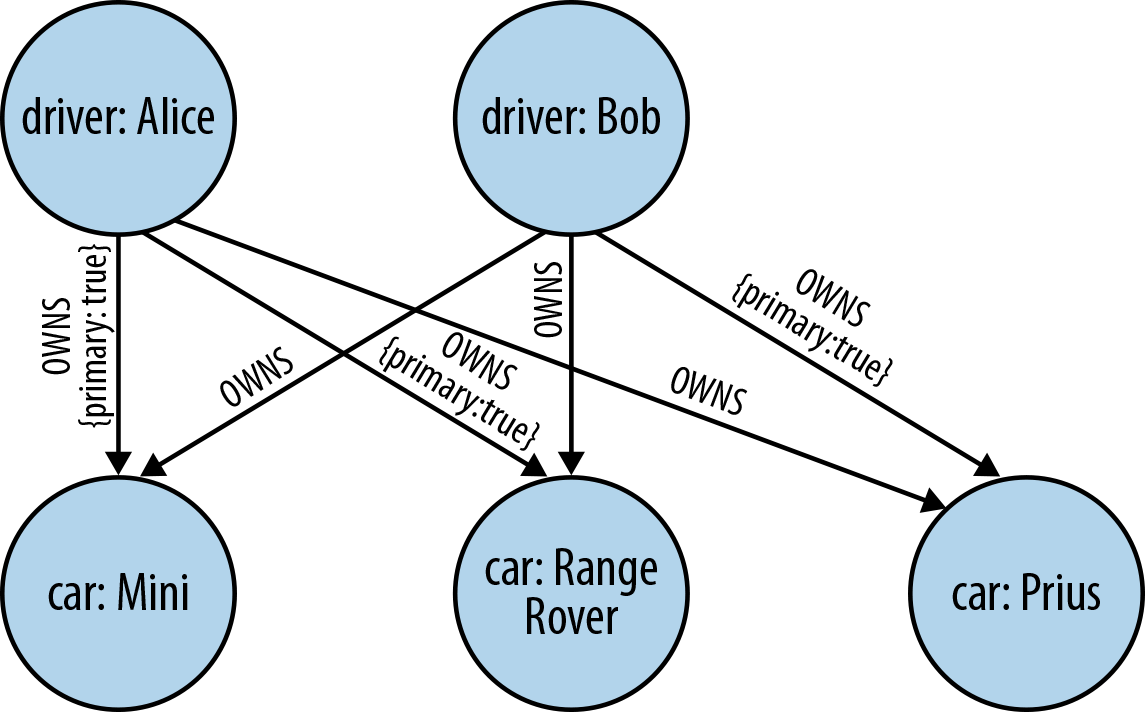
Figure A-8. A property graph is semantically fine-tuned

Note

Because hyper-edges are multidimensional, hypergraphs comprise a more general model than property graphs. That said, the two models are isomorphic. It is always possible to represent the information in a hypergraph as a property graph (albeit using more relationships and intermediary nodes). Whether a hypergraph or a property graph is best for you is going to depend on your modeling mindset and the kinds of applications you’re building. Anecdotally, for most purposes property graphs are widely considered to have the best balance of pragmatism and modeling efficiency—hence their overwhelming popularity in the graph database space. However, in situations where you need to capture meta-intent, effectively qualifying one relationship with another (e.g., I like the fact that you liked that car), hypergraphs typically require fewer primitives than property graphs.

<rdf:RDF xmlns:rdf="http://www.w3.org/1999/02/22-rdf-syntax-ns#"
         xmlns="http://www.example.org/terms/">
	<rdf:Description rdf:about="http://www.example.org/ginger">
		<name>Ginger Rogers</name>
		<occupation>dancer</occupation>
		<partner rdf:resource="http://www.example.org/fred"/>
	</rdf:Description>
	<rdf:Description rdf:about="http://www.example.org/fred">
		<name>Fred Astaire</name>
		<occupation>dancer</occupation>
		<likes rdf:resource="http://www.example.org/ice-cream"/>
	</rdf:Description>
</rdf:RDF>