
Chapter 3. Data Modeling with Graphs
In previous chapters we’ve described the substantial benefits of the graph database when compared both with other NOSQL stores and with traditional relational databases. But having chosen to adopt a graph database, the question arises: how do we model in graphs?
This chapter focuses on graph modeling. Starting with a recap of the labeled property graph model—the most widely adopted graph data model—we then provide an overview of the graph query language used for most of the code examples in this book: Cypher. Though there are several graph query languages in existence, Cypher is the most widely deployed, making it the de facto standard. It is also easy to learn and understand, especially for those of us coming from a SQL background. With these fundamentals in place, we dive straight into some examples of graph modeling. With our first example, based on a systems management domain, we compare relational and graph modeling techniques. In the second example, the production and consumption of Shakespearean literature, we use a graph to connect and query several disparate domains. We end the chapter by looking at some common pitfalls when modeling with graphs, and highlight some good practices.
Models and Goals
Before we dig deeper into modeling with graphs, a word on models in general. Modeling is an abstracting activity motivated by a particular need or goal. We model in order to bring specific facets of an unruly domain into a space where they can be structured and manipulated. There are no natural representations of the world the way it “really is,” just many purposeful selections, abstractions, and simplifications, some of which are more useful than others for satisfying a particular goal.
Graph representations are no different in this respect. What perhaps differentiates them from many other data modeling techniques, however, is the close affinity between the logical and physical models. Relational data management techniques require us to deviate from our natural language representation of the domain: first by cajoling our representation into a logical model, and then by forcing it into a physical model. These transformations introduce semantic dissonance between our conceptualization of the world and the database’s instantiation of that model. With graph databases, this gap shrinks considerably.
The Labeled Property Graph Model
We introduced the labeled property graph model in Chapter 1. To recap, these are its salient features:
-
A labeled property graph is made up of nodes, relationships, properties, and labels.
-
Nodes contain properties. Think of nodes as documents that store properties in the form of arbitrary key-value pairs. In Neo4j, the keys are strings and the values are the Java string and primitive data types, plus arrays of these types.
-
Nodes can be tagged with one or more labels. Labels group nodes together, and indicate the roles they play within the dataset.
-
Relationships connect nodes and structure the graph. A relationship always has a direction, a single name, and a start node and an end node—there are no dangling relationships. Together, a relationship’s direction and name add semantic clarity to the structuring of nodes.
-
Like nodes, relationships can also have properties. The ability to add properties to relationships is particularly useful for providing additional metadata for graph algorithms, adding additional semantics to relationships (including quality and weight), and for constraining queries at runtime.
These simple primitives are all we need to create sophisticated and semantically rich models. So far, all our models have been in the form of diagrams. Diagrams are great for describing graphs outside of any technology context, but when it comes to using a database, we need some other mechanism for creating, manipulating, and querying data. We need a query language.
Querying Graphs: An Introduction to Cypher
Cypher is an expressive (yet compact) graph database query language. Although currently specific to Neo4j, its close affinity with our habit of representing graphs as diagrams makes it ideal for programmatically describing graphs. For this reason, we use Cypher throughout the rest of this book to illustrate graph queries and graph constructions. Cypher is arguably the easiest graph query language to learn, and is a great basis for learning about graphs. Once you understand Cypher, it becomes very easy to branch out and learn other graph query languages.
In the following sections we’ll take a brief tour through Cypher. This isn’t a reference document for Cypher, however—merely a friendly introduction so that we can explore more interesting graph query scenarios later on.1
Cypher Philosophy
Cypher is designed to be easily read and understood by developers, database professionals, and business stakeholders. Its ease of use derives from the fact that it is in accord with the way we intuitively describe graphs using diagrams.
Cypher enables a user (or an application acting on behalf of a user) to ask the database to find data that matches a specific pattern. Colloquially, we ask the database to “find things like this.” And the way we describe what “things like this” look like is to draw them, using ASCII art. Figure 3-1 shows an example of a simple pattern.

Figure 3-1. A simple graph pattern, expressed using a diagram
This pattern describes three mutual friends. Here’s the equivalent ASCII art representation in Cypher:
(emil)<-[:KNOWS]-(jim)-[:KNOWS]->(ian)-[:KNOWS]->(emil)This pattern describes a path that connects a node we’ll call jim to two nodes we’ll call ian and emil, and which also connects the ian node to the emil node. ian, jim, and emil are identifers. Identifiers allow us to refer to the same node more than once when describing a pattern—a trick that helps us get round the fact that a query language has only one dimension (text proceeding from left to right), whereas a graph diagram can be laid out in two dimensions. Despite having occasionally to repeat identifiers in this way, the intent remains clear. Cypher patterns follow very naturally from the way we draw graphs on the whiteboard.
Note
The previous Cypher pattern describes a simple graph structure, but it doesn’t yet refer to any particular data in the database. To bind the pattern to specific nodes and relationships in an existing dataset we must specify some property values and node labels that help locate the relevant elements in the dataset. For example:
(emil:Person {name:'Emil'})<-[:KNOWS]-(jim:Person {name:'Jim'})-[:KNOWS]->(ian:Person {name:'Ian'})-[:KNOWS]->(emil)
Here we’ve bound each node to its identifier using its name property and Person label. The emil identifer, for example, is bound to a node in the dataset with a label Person and a name property whose value is Emil. Anchoring parts of the pattern to real data in this way is normal Cypher practice, as we shall see in the following sections.
ASCII art graph patterns are fundamental to Cypher. A Cypher query anchors one or more parts of a pattern to specific locations in a graph using predicates, and then flexes the unanchored parts around to find local matches.
Note
The anchor points in the real graph, to which some parts of the pattern are bound, are determined by Cypher based on the labels and property predicates in the query. In most cases, Cypher uses metainformation about existing indexes, constraints, and predicates to figure things out automatically. Occasionally, however, it helps to specify some additional hints.
Like most query languages, Cypher is composed of clauses. The simplest queries consist of a MATCH clause followed by a RETURN clause (we’ll describe the other clauses you can use in a Cypher query later in this chapter). Here’s an example of a Cypher query that uses these three clauses to find the mutual friends of a user named Jim:
MATCH(a:Person {name:'Jim'})-[:KNOWS]->(b)-[:KNOWS]->(c),(a)-[:KNOWS]->(c)RETURNb, c
Let’s look at each clause in more detail.
MATCH
The MATCH clause is at the heart of most Cypher queries. This is the specification by example part. Using ASCII characters to represent nodes and relationships, we draw the data we’re interested in. We draw nodes with parentheses, and relationships using pairs of dashes with greater-than or less-than signs (--> and <--). The < and > signs indicate relationship direction. Between the dashes, set off by square brackets and prefixed by a colon, we put the relationship name. Node labels are similarly prefixed by a colon. Node (and relationship) property key-value pairs are then specified within curly braces (much like a Javascript object).
In our example query, we’re looking for a node labeled Person with a name property whose value is Jim. The return value from this lookup is bound to the identifier a. This identifier allows us to refer to the node that represents Jim throughout the rest of the query.
This start node is part of a simple pattern (a)-[:KNOWS]->(b)-[:KNOWS]->(c), (a)-[:KNOWS]->(c) that describes a path comprising three nodes, one of which we’ve bound to the identifier a, the others to b and c. These nodes are connected by way of several KNOWS relationships, as per Figure 3-1.
This pattern could, in theory, occur many times throughout our graph data; with a large user set, there may be many mutual relationships corresponding to this pattern. To localize the query, we need to anchor some part of it to one or more places in the graph. In specifying that we’re looking for a node labeled Person whose name property value is Jim, we’ve bound the pattern to a specific node in the graph—the node representing Jim. Cypher then matches the remainder of the pattern to the graph immediately surrounding this anchor point. As it does so, it discovers nodes to bind to the other identifiers. While a will always be anchored to Jim, b and c will be bound to a sequence of nodes as the query executes.
Alternatively, we can express the anchoring as a predicate in the WHERE clause.
MATCH(a:Person)-[:KNOWS]->(b)-[:KNOWS]->(c), (a)-[:KNOWS]->(c)WHEREa.name ='Jim'RETURNb, c
Here we’ve moved the property lookup from the MATCH clause to the WHERE clause. The outcome is the same as our earlier query.
RETURN
This clause specifies which nodes, relationships, and properties in the matched data should be returned to the client. In our example query, we’re interested in returning the nodes bound to the b and c identifiers. Each matching node is lazily bound to its identifier as the client iterates the results.
Other Cypher Clauses
The other clauses we can use in a Cypher query include:
WHERECREATEandCREATE UNIQUEMERGE-
Ensures that the supplied pattern exists in the graph, either by reusing existing nodes and relationships that match the supplied predicates, or by creating new nodes and relationships.
DELETESETFOREACHUNIONWITH-
Chains subsequent query parts and forwards results from one to the next. Similar to piping commands in Unix.
START-
Specifies one or more explicit starting points—nodes or relationships—in the graph. (
STARTis deprecated in favor of specifying anchor points in aMATCHclause.)
If these clauses look familiar—especially if you’re a SQL developer—that’s great! Cypher is intended to be familiar enough to help you move rapidly along the learning curve. At the same time, it’s different enough to emphasize that we’re dealing with graphs, not relational sets.
We’ll see some examples of these clauses later in the chapter. Where they occur, we’ll describe in more detail how they work.
Now that we’ve seen how we can describe and query a graph using Cypher, we can look at some examples of graph modeling.
A Comparison of Relational and Graph Modeling
To introduce graph modeling, we’re going to look at how we model a domain using both relational- and graph-based techniques. Most developers and data professionals are familiar with RDBMS (relational database management systems) and the associated data modeling techniques; as a result, the comparison will highlight a few similarities, and many differences. In particular, we’ll see how easy it is to move from a conceptual graph model to a physical graph model, and how little the graph model distorts what we’re trying to represent versus the relational model.
To facilitate this comparison, we’ll examine a simple data center management domain. In this domain, several data centers support many applications on behalf of many customers using different pieces of infrastructure, from virtual machines to physical load balancers. An example of this domain is shown in Figure 3-2.
In Figure 3-2 we see a somewhat simplified view of several applications and the data center infrastructure necessary to support them. The applications, represented by nodes App 1, App 2, and App 3, depend on a cluster of databases labeled Database Server 1, 2, 3. While users logically depend on the availability of an application and its data, there is additional physical infrastructure between the users and the application; this infrastructure includes virtual machines (Virtual Machine 10, 11, 20, 30, 31), real servers (Server 1, 2, 3), racks for the servers (Rack 1, 2 ), and load balancers (Load Balancer 1, 2), which front the apps. In between each of the components there are, of course, many networking elements: cables, switches, patch panels, NICs (network interface controllers), power supplies, air conditioning, and so on—all of which can fail at inconvenient times. To complete the picture we have a straw-man single user of application 3, represented by User 3.
As the operators of such a system, we have two primary concerns:
-
Ongoing provision of functionality to meet (or exceed) a service-level agreement, including the ability to perform forward-looking analyses to determine single points of failure, and retrospective analyses to rapidly determine the cause of any customer complaints regarding the availability of service.
-
Billing for resources consumed, including the cost of hardware, virtualization, network provisioning, and even the costs of software development and operations (since these are simply logical extensions of the system we see here).
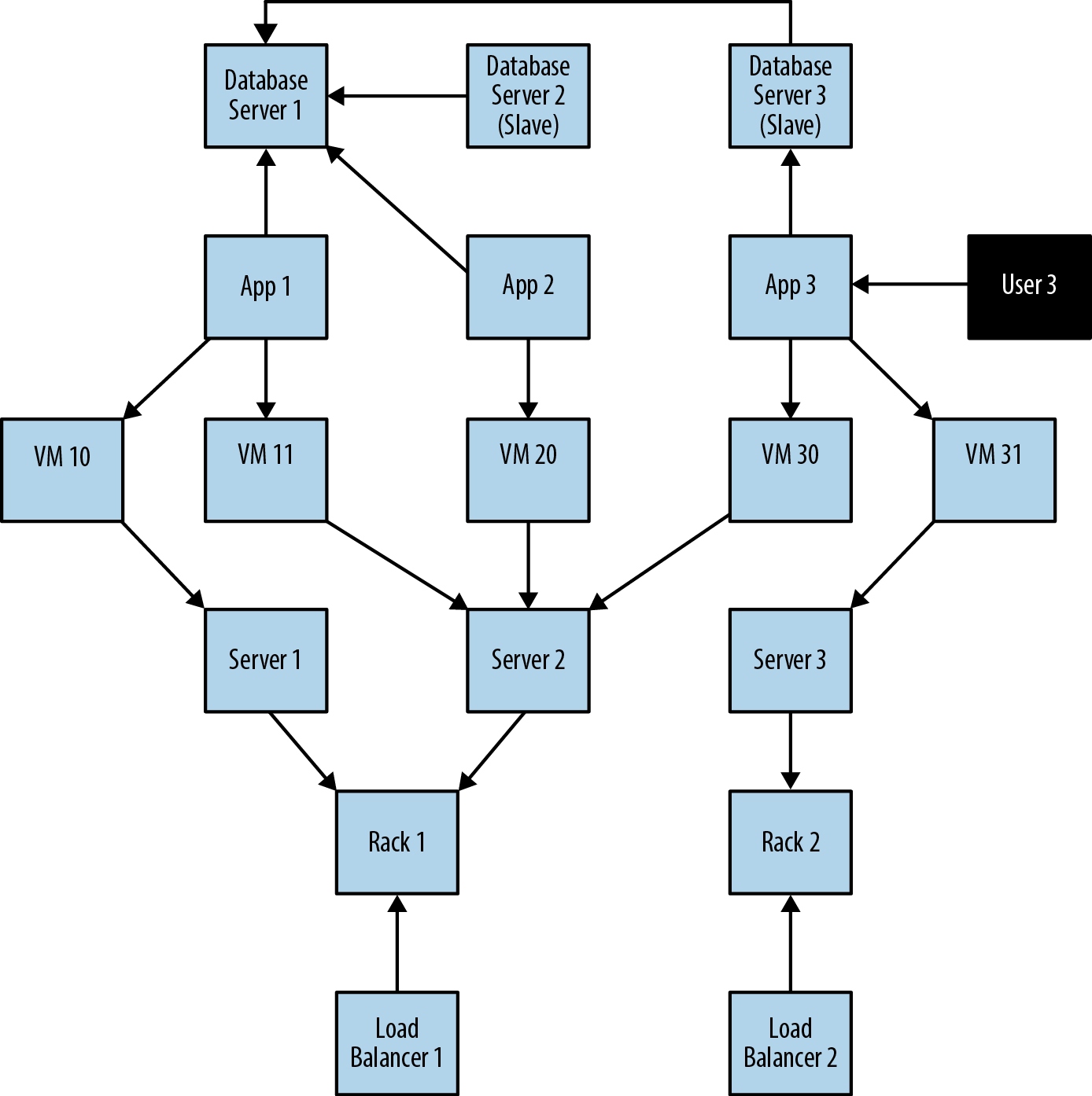
Figure 3-2. Simplified snapshot of application deployment within a data center
If we are building a data center management solution, we’ll want to ensure that the underlying data model allows us to store and query data in a way that efficiently addresses these primary concerns. We’ll also want to be able to update the underlying model as the application portfolio changes, the physical layout of the data center evolves, and virtual machine instances migrate. Given these needs and constraints, let’s see how the relational and graph models compare.
Relational Modeling in a Systems Management Domain
The initial stage of modeling in the relational world is similar to the first stage of many other data modeling techniques: that is, we seek to understand and agree on the entities in the domain, how they interrelate, and the rules that govern their state transitions. Most of this tends to be done informally, often through whiteboard sketches and discussions between subject matter experts and systems and data architects. To express our common understanding and agreement, we typically create a diagram such as the one in Figure 3-2, which is a graph.
The next stage captures this agreement in a more rigorous form such as an entity-relationship (E-R) diagram—another graph. This transformation of the conceptual model into a logical model using a stricter notation provides us with a second chance to refine our domain vocabulary so that it can be shared with relational database specialists. (Such approaches aren’t always necessary: adept relational users often move directly to table design and normalization without first describing an intermediate E-R diagram.) In our example, we’ve captured the domain in the E-R diagram shown in Figure 3-3.
Note
Despite being graphs, E-R diagrams immediately demonstrate the shortcomings of the relational model for capturing a rich domain. Although they allow relationships to be named (something that graph databases fully embrace, but which relational stores do not), E-R diagrams allow only single, undirected, named relationships between entities. In this respect, the relational model is a poor fit for real-world domains where relationships between entities are both numerous and semantically rich and diverse.
Having arrived at a suitable logical model, we map it into tables and relations, which are normalized to eliminate data redundancy. In many cases this step can be as simple as transcribing the E-R diagram into a tabular form and then loading those tables via SQL commands into the database. But even the simplest case serves to highlight the idiosyncrasies of the relational model. For example, in Figure 3-4 we see that a great deal of accidental complexity has crept into the model in the form of foreign key constraints (everything annotated [FK]), which support one-to-many relationships, and join tables (e.g., AppDatabase), which support many-to-many relationships—and all this before we’ve added a single row of real user data. These constraints are model-level metadata that exist simply so that we can make concrete the relations between tables at query time. Yet the presence of this structural data is keenly felt, because it clutters and obscures the domain data with data that serves the database, not the user.

Figure 3-3. An entity-relationship diagram for the data center domain
We now have a normalized model that is relatively faithful to the domain. This model, though imbued with substantial accidental complexity in the form of foreign keys and join tables, contains no duplicate data. But our design work is not yet complete. One of the challenges of the relational paradigm is that normalized models generally aren’t fast enough for real-world needs. For many production systems, a normalized schema, which in theory is fit for answering any kind of ad hoc question we may wish to pose to the domain, must in practice be further adapted and specialized for specific access patterns. In other words, to make relational stores perform well enough for regular application needs, we have to abandon any vestiges of true domain affinity and accept that we have to change the user’s data model to suit the database engine, not the user. This technique is called denormalization.
Denormalization involves duplicating data (substantially in some cases) in order to gain query performance. Take as an example users and their contact details. A typical user often has several email addresses, which, in a fully normalized model, we would store in a separate EMAIL table. To reduce joins and the performance penalty imposed by joining between two tables, however, it is quite common to inline this data in the USER table, adding one or more columns to store a user’s most important email addresses.

Figure 3-4. Tables and relationships for the data center domain
Although denormalization may be a safe thing to do (assuming developers understand the denormalized model and how it maps to their domain-centric code, and have robust transactional support from the database), it is usually not a trivial task. For the best results, we usually turn to a true RDBMS expert to munge our normalized model into a denormalized one aligned with the characteristics of the underlying RDBMS and physical storage tier. In doing this, we accept that there may be substantial data redundancy.
We might be tempted to think that all this design-normalize-denormalize effort is acceptable because it is a one-off task. This school of thought suggests that the cost of the work is amortized across the entire lifetime of the system (which includes both development and production) such that the effort of producing a performant relational model is comparatively small compared to the overall cost of the project. This is an appealing notion, but in many cases it doesn’t match reality, because systems change not only during development, but also during their production lifetimes.
The amortized view of data model change, in which costly changes during development are eclipsed by the long-term benefits of a stable model in production, assumes that systems spend the majority of their time in production environments, and that these production environments are stable. Though it may be the case that most systems spend most of their time in production environments, these environments are rarely stable. As business requirements change or regulatory requirements evolve, so must our systems and the data structures on which they are built.
Data models invariably undergo substantial revision during the design and development phases of a project, and in almost every case, these revisions are intended to accommodate the model to the needs of the applications that will consume it once it is in production. These initial design influences are so powerful that it becomes nearly impossible to modify the application and the model once they’re in production to accommodate things they were not originally designed to do.
The technical mechanism by which we introduce structural change into a database is called migration, as popularized by application development frameworks such as Rails. Migrations provide a structured, step-wise approach to applying a set of database refactorings to a database so that it can be responsibly evolved to meet the changing needs of the applications that use it. Unlike code refactorings, however, which we typically accomplish in a matter of seconds or minutes, database refactorings can take weeks or months to complete, with downtime for schema changes. Database refactoring is slow, risky, and expensive.
The problem, then, with the denormalized model is its resistance to the kind of rapid evolution the business demands of its systems. As we’ve seen with the data center example, the changes imposed on the whiteboard model over the course of implementing a relational solution create a gulf between the conceptual world and the way the data is physically laid out; this conceptual-relational dissonance all but prevents business stakeholders from actively collaborating in the further evolution of a system. Stakeholder participation stops at the threshold of the relational edifice. On the development side, the difficulties in translating changed business requirements into the underlying and entrenched relational structure cause the evolution of the system to lag behind the evolution of the business. Without expert assistance and rigorous planning, migrating a denormalized database poses several risks. If the migrations fail to maintain storage-affinity, performance can suffer. Just as serious, if deliberately duplicated data is left orphaned after a migration, we risk compromising the integrity of the data as a whole.
Graph Modeling in a Systems Management Domain
We’ve seen how relational modeling and its attendant implementation activities take us down a path that divorces an application’s underlying storage model from the conceptual worldview of its stakeholders. Relational databases—with their rigid schemas and complex modeling characteristics—are not an especially good tool for supporting rapid change. What we need is a model that is closely aligned with the domain, but that doesn’t sacrifice performance, and that supports evolution while maintaining the integrity of the data as it undergoes rapid change and growth. That model is the graph model. How, then, does this process differ when realized with a graph data model?
In the early stages of analysis, the work required of us is similar to the relational approach: using lo-fi methods, such as whiteboard sketches, we describe and agree upon the domain. After that, however, the methodologies diverge. Instead of transforming a domain model’s graph-like representation into tables, we enrich it, with the aim of producing an accurate representation of the parts of the domain relevant to our application goals. That is, for each entity in our domain, we ensure that we’ve captured its relevant roles as labels, its attributes as properties, and its connections to neighboring entities as relationships.
Note
Remember, the domain model is not a transparent, context-free window onto reality: rather, it is a purposeful abstraction of those aspects of our domain relevant to our application goals. There’s always some motivation for creating a model. By enriching our first-cut domain graph with additional properties and relationships, we effectively produce a graph model attuned to our application’s data needs; that is, we provide for answering the kinds of questions our application will ask of its data.
Helpfully, domain modeling is completely isomorphic to graph modeling. By ensuring the correctness of the domain model, we’re implicitly improving the graph model, because in a graph database what you sketch on the whiteboard is typically what you store in the database.
In graph terms, what we’re doing is ensuring that each node has the appropriate role-specific labels and properties so that it can fulfill its dedicated data-centric domain responsibilities. But we’re also ensuring that every node is placed in the correct semantic context; we do this by creating named and directed (and often attributed) relationships between nodes to capture the structural aspects of the domain. For our data center scenario, the resulting graph model looks like Figure 3-5.

Figure 3-5. Example graph for the data center deployment scenario
And logically, that’s all we need to do. No tables, no normalization, no denormalization. Once we have an accurate representation of our domain model, moving it into the database is trivial, as we shall see shortly.
Note
Note that most of the nodes here have two labels: both a specific type label (such as Database, App, or Server), and a more general-purpose Asset label. This allows us to target particular types of asset with some of our queries, and all assets, irrespective of type, with other queries.
Testing the Model
Once we’ve refined our domain model, the next step is to test how suitable it is for answering realistic queries. Although graphs are great for supporting a continuously evolving structure (and therefore for correcting any erroneous earlier design decisions), there are a number of design decisions that, once they are baked into our application, can hamper us further down the line. By reviewing the domain model and the resulting graph model at this early stage, we can avoid these pitfalls. Subsequent changes to the graph structure will then be driven solely by changes in the business, rather than by the need to mitigate poor design decisions.
In practice there are two techniques we can apply here. The first, and simplest, is just to check that the graph reads well. We pick a start node, and then follow relationships to other nodes, reading each node’s labels and each relationship’s name as we go. Doing so should create sensible sentences. For our data center example, we can read off sentences like “The App, which consists of App Instances 1, 2, and 3, uses the Database, which resides on Database Servers 1, 2 and 3,” and “Server 3 runs VM 31, which hosts App Instance 3.” If reading the graph in this way makes sense, we can be reasonably confident it is faithful to the domain.
To further increase our confidence, we also need to consider the queries we’ll run on the graph. Here we adopt a design for queryability mindset. To validate that the graph supports the kinds of queries we expect to run on it, we must describe those queries. This requires us to understand our end users’ goals; that is, the use cases to which the graph is to be applied. In our data center scenario, for example, one of our use cases involves end users reporting that an application or service is unresponsive. To help these users, we must identify the cause of the unresponsiveness and then resolve it. To determine what might have gone wrong we need to identify what’s on the path between the user and the application, and also what the application depends on to deliver functionality to the user. Given a particular graph representation of the data center domain, if we can craft a Cypher query that addresses this use case, we can be even more certain that the graph meets the needs of our domain.
Continuing with our example use case, let’s assume we can update the graph from our regular network monitoring tools, thereby providing us with a near real-time view of the state of the network. With a large physical network, we might use Complex Event Processing (CEP) to process streams of low-level network events, updating the graph only when the CEP solution raises a significant domain event. When a user reports a problem, we can limit the physical fault-finding to problematic network elements between the user and the application and the application and its dependencies. In our graph we can find the faulty equipment with the following query:
MATCH(user:User)-[*1..5]-(asset:Asset)WHEREuser.name ='User 3'ANDasset.status ='down'RETURN DISTINCTasset
The MATCH clause here describes a variable length path between one and five relationships long. The relationships are unnamed and undirected (there’s no colon or relationship name between the square brackets, and no arrow-tip to indicate direction). This allows us to match paths such as:
(user)-[:USER_OF]->(app)(user)-[:USER_OF]->(app)-[:USES]->(database)(user)-[:USER_OF]->(app)-[:USES]->(database)-[:SLAVE_OF]->(another-database)(user)-[:USER_OF]->(app)-[:RUNS_ON]->(vm)(user)-[:USER_OF]->(app)-[:RUNS_ON]->(vm)-[:HOSTED_BY]->(server)(user)-[:USER_OF]->(app)-[:RUNS_ON]->(vm)-[:HOSTED_BY]->(server)-[:IN]->(rack)(user)-[:USER_OF]->(app)-[:RUNS_ON]->(vm)-[:HOSTED_BY]->(server)-[:IN]->(rack)<-[:IN]-(load-balancer)
That is, starting from the user who reported the problem, we MATCH against all assets in the graph along an undirected path of length 1 to 5. We add asset nodes that have a status property with a value of down to our results. If a node doesn’t have a status property, it won’t be included in the results. RETURN DISTINCT asset ensures that unique assets are returned in the results, no matter how many times they are matched.
Given that such a query is readily supported by our graph, we gain confidence that the design is fit for purpose.
Cross-Domain Models
Business insight often depends on us understanding the hidden network effects at play in a complex value chain. To generate this understanding, we need to join domains together without distorting or sacrificing the details particular to each domain. Property graphs provide a solution here. Using a property graph, we can model a value chain as a graph of graphs in which specific relationships connect and distinguish constituent subdomains.
In Figure 3-6, we see a graph representation of the value chain surrounding the production and consumption of Shakespearean literature. Here we have high-quality information about Shakespeare and some of his plays, together with details of one of the companies that has recently performed the plays, plus a theatrical venue, and some geospatial data. We’ve even added a review. In all, the graph describes and connects three different domains. In the diagram we’ve distinguished these three domains with differently formatted relationships: dotted for the literary domain, solid for the theatrical domain, and dashed for the geospatial domain.
Looking first at the literary domain, we have a node that represents Shakespeare himself, with a label Author and properties firstname:'William' and lastname:'Shakespeare'. This node is connected to a pair of nodes, each of which is labeled Play, representing the plays Julius Caesar (title:'Julius Caesar') and The Tempest (title:'The Tempest'), via relationships named WROTE_PLAY.

Figure 3-6. Three domains in one graph
Reading this subgraph left-to-right, following the direction of the relationship arrows, tells us that the author William Shakespeare wrote the plays Julius Caesar and The Tempest. If we’re interested in provenance, each WROTE_PLAY relationship has a date property, which tells us that Julius Caesar was written in 1599 and The Tempest in 1610. It’s a trivial matter to see how we could add the rest of Shakespeare’s works—the plays and the poems—into the graph simply by adding more nodes to represent each work, and joining them to the Shakespeare node via WROTE_PLAY and WROTE_POEM relationships.
Note
By tracing the WROTE_PLAY relationship arrows with our finger, we’re effectively doing the kind of work that a graph database performs, albeit at human speed rather than computer speed. As we’ll see later, this simple traversal operation is the building block for arbitrarily sophisticated graph queries.
Turning next to the theatrical domain, we’ve added some information about the Royal Shakespeare Company (often known simply as the RSC) in the form of a node with the label Company and a property key name whose value is RSC. The theatrical domain is, unsurprisingly, connected to the literary domain. In our graph, this is reflected by the fact that the RSC has PRODUCED versions of Julius Caesar and The Tempest. In turn, these theatrical productions are connected to the plays in the literary domain, using PRODUCTION_OF relationships.
The graph also captures details of specific performances. For example, the RSC’s production of Julius Caesar was performed on July 29, 2012 as part of the RSC’s summer touring season. If we’re interested in the performance venue, we simply follow the outgoing VENUE relationship from the performance node to find that the play was performed at the Theatre Royal, represented by a node labeled Venue.
The graph also allows us to capture reviews of specific performances. In our sample graph we’ve included just one review, for the July 29 performance, written by the user Billy. We can see this in the interplay of the performance, rating, and user nodes. In this case we have a node labeled User representing Billy (with property name:'Billy') whose outgoing WROTE_REVIEW relationship connects to a node representing his review. The Review node contains a numeric rating property and a free-text review property. The review is linked to a specific Performance through an outgoing REVIEW_OF relationship. To scale this up to many users, many reviews, and many performances, we simply add more nodes with the appropriate labels and more identically named relationships to the graph.
The third domain, that of geospatial data, comprises a simple hierarchical tree of places. This geospatial domain is connected to the other two domains at several points in the graph. The City of Stratford upon Avon (with property name:'Stratford upon Avon') is connected to the literary domain as a result of its being Shakespeare’s birthplace (Shakespeare was BORN_IN Stratford). It is connected to the theatrical domain insofar as it is home to the RSC (the RSC is BASED_IN Stratford). To learn more about Stratford upon Avon’s geography, we can follow its outgoing COUNTRY relationship to discover it is in the Country named England.
Note
Note how the graph reduces instances of duplicated data across domains. Stratford upon Avon, for example, participates in all three domains.
The graph makes it possible to capture more complex geospatial data. Looking at the labels on the nodes to which the Theatre Royal is connected, for example, we see that it is located on Grey Street, which is in the City of Newcastle, which is in the County of Tyne and Wear, which ultimately is in the Country of England—just like Stratford upon Avon.
Creating the Shakespeare Graph
To create the Shakespeare graph shown in Figure 3-6, we use CREATE to build the overall structure. This statement is executed by the Cypher runtime within a single transaction such that once the statement has executed, we can be confident the graph is present in its entirety in the database. If the transaction fails, no part of the graph will be present in the database. As we might expect, Cypher has a humane and visual way of building graphs:
CREATE(shakespeare:Author {firstname:'William', lastname:'Shakespeare'}),(juliusCaesar:Play {title:'Julius Caesar'}),(shakespeare)-[:WROTE_PLAY {year:1599}]->(juliusCaesar),(theTempest:Play {title:'The Tempest'}),(shakespeare)-[:WROTE_PLAY {year:1610}]->(theTempest),(rsc:Company {name:'RSC'}),(production1:Production {name:'Julius Caesar'}),(rsc)-[:PRODUCED]->(production1),(production1)-[:PRODUCTION_OF]->(juliusCaesar),(performance1:Performance {date:20120729}),(performance1)-[:PERFORMANCE_OF]->(production1),(production2:Production {name:'The Tempest'}),(rsc)-[:PRODUCED]->(production2),(production2)-[:PRODUCTION_OF]->(theTempest),(performance2:Performance {date:20061121}),(performance2)-[:PERFORMANCE_OF]->(production2),(performance3:Performance {date:20120730}),(performance3)-[:PERFORMANCE_OF]->(production1),(billy:User {name:'Billy'}),(review:Review {rating:5, review:'This was awesome!'}),(billy)-[:WROTE_REVIEW]->(review),(review)-[:RATED]->(performance1),(theatreRoyal:Venue {name:'Theatre Royal'}),(performance1)-[:VENUE]->(theatreRoyal),(performance2)-[:VENUE]->(theatreRoyal),(performance3)-[:VENUE]->(theatreRoyal),(greyStreet:Street {name:'Grey Street'}),(theatreRoyal)-[:STREET]->(greyStreet),(newcastle:City {name:'Newcastle'}),(greyStreet)-[:CITY]->(newcastle),(tyneAndWear:County {name:'Tyne and Wear'}),(newcastle)-[:COUNTY]->(tyneAndWear),(england:Country {name:'England'}),(tyneAndWear)-[:COUNTRY]->(england),(stratford:City {name:'Stratford upon Avon'}),(stratford)-[:COUNTRY]->(england),(rsc)-[:BASED_IN]->(stratford),(shakespeare)-[:BORN_IN]->stratford
The preceding Cypher code does two different things. It creates labeled nodes (and their properties), and then connects them with relationships (and their relationship properties where necessary). For example, CREATE (shakespeare:Author {firstname:'William', lastname:'Shakespeare'}) creates an Author node representing William Shakespeare. The newly created node is assigned to the identifier shakespeare. This shakespeare identifier is used later in the code to attach relationships to the underlying node. For example, (shakespeare)-[:WROTE_PLAY {year:1599}]->(juliusCaesar) creates a WROTE relationship from Shakespeare to the play Julius Caesar. This relationship has a year property with value 1599.
Identifiers remain available for the duration of the current query scope, but no longer. Should we wish to give long-lived names to nodes, we simply create an index for a particular label and key property combination. We discuss indexes in see “Indexes and Constraints”.
Note
Unlike the relational model, these commands don’t introduce any accidental complexity into the graph. The information meta-model—that is, the structuring of nodes through labels and relationships—is kept separate from the business data, which lives exclusively as properties. We no longer have to worry about foreign key and cardinality constraints polluting our real data, because both are explicit in the graph model in the form of nodes and the semantically rich relationships that interconnect them.
We can modify the graph at a later point in time in two different ways. We can, of course, continue using CREATE statements to simply add to the graph. But we can also use MERGE, which has the semantics of ensuring that a particular subgraph structure of nodes and relationships—some of which may already exist, some of which may be missing—is in place once the command has executed. In practice, we tend to use CREATE when we’re adding to the graph and don’t mind duplication, and MERGE when duplication is not permitted by the domain.
Beginning a Query
Now that we have a graph, we can start to query it. In Cypher we always begin our queries from one or more well-known starting points in the graph—what are called bound nodes. Cypher uses any labels and property predicates supplied in the MATCH and WHERE clauses, together with metadata supplied by indexes and constraints, to find the starting points that anchor our graph patterns.
For instance, if we wanted to discover more about performances at the Theatre Royal, we’d start our query from the Theatre Royal node, which we find by specifying its Venue label and name property. If, however, we were more interested in a person’s reviews, we’d use that person’s node as a starting point for our query, matching on the User label and name property combination.
Let’s assume we want to find out about all the Shakespeare events that have taken place in the Theatre Royal in Newcastle. These three things—an Author named Shakespeare, a Venue called Theatre Royal, and a City with the name Newcastle—provide the starting points for our new query:
MATCH(theater:Venue {name:'Theatre Royal'}),(newcastle:City {name:'Newcastle'}),(bard:Author {lastname:'Shakespeare'})
This MATCH clause identifies all Venue nodes with a property key name and property value Theatre Royal and binds them to the identifier theater. (What if there are many Theatre Royal nodes in this graph? We’ll deal with that shortly.) As the next step, we find the node representing the City of Newcastle; we bind this node to the identifier newcastle. Finally, as with our earlier Shakespeare query, to find the Shakespeare node itself, we look for a node with the label Author and a lastname property whose value is Shakespeare. We bind the result of this lookup to bard.
From now on in our query, wherever we use the identifiers theater, newcastle, and bard in a pattern, that pattern will be anchored to the real nodes associated with these three identifiers. In effect, this information binds the query to a specific part of the graph, giving us starting points from which to match patterns in the immediately surrounding nodes and relationships.
Declaring Information Patterns to Find
The MATCH clause in Cypher is where the magic happens. As much as the CREATE clause tries to convey intent using ASCII art to describe the desired state of the graph, so the MATCH clause uses the same syntax to describe patterns to discover in the database. We’ve already looked at a very simple MATCH clause; now we’ll look at a more complex pattern that finds all the Shakespeare performances at Newcastle’s Theatre Royal:
MATCH(theater:Venue {name:'Theatre Royal'}),(newcastle:City {name:'Newcastle'}),(bard:Author {lastname:'Shakespeare'}),(newcastle)<-[:STREET|CITY*1..2]-(theater)<-[:VENUE]-()-[:PERFORMANCE_OF]->()-[:PRODUCTION_OF]->(play)<-[:WROTE_PLAY]-(bard)RETURN DISTINCTplay.titleASplay
This MATCH pattern uses several syntactic elements we’ve not yet come across. As well as anchored nodes that we discussed earlier, it uses pattern nodes, arbitrary depth paths, and anonymous nodes. Let’s take a look at each of these in turn:
-
The identifiers
newcastle,theater, andbardare anchored to real nodes in the graph based on the specified label and property values. -
If there are several Theatre Royals in our database (the British cities of Plymouth, Bath, Winchester, and Norwich all have a Theatre Royal, for example), then
theaterwill be bound to all these nodes. To restrict our pattern to the Theatre Royal in Newcastle, we use the syntax<-[:STREET|CITY*1..2]-, which means thetheaternode can be no more than two outgoingSTREETand/orCITYrelationships away from the node representing the city of Newcastle-upon-Tyne. By providing a variable depth path, we allow for relatively fine-grained address hierarchies (comprising, for example, street, district or borough, and city). -
The syntax
(theater)<-[:VENUE]-()uses the anonymous node, hence the empty parentheses. Knowing the data as we do, we expect the anonymous node to match performances, but because we’re not interested in using the details of individual performances elsewhere in the query or in the results, we don’t name the node or bind it to an identifier. -
We use the anonymous node again to link the performance to the production (
()-[:PERFORMANCE_OF]->()). If we were interested in returning details of performances and productions, we would replace these occurrences of the anonymous node with identifiers:(performance)-[:PERFORMANCE_OF]->(production). -
The remainder of the
MATCHis a straightforward(play)<-[:WROTE_PLAY]-(bard)node-to-relationship-to-node pattern match. This pattern ensures that we only return plays written by Shakespeare. Because(play)is joined to the anonymous production node, and by way of that to the performance node, we can safely infer that it has been performed in Newcastle’s Theatre Royal. In naming the play node we bring it into scope so that we can use it later in the query.
Running this query returns all the Shakespeare plays that have been performed at the Theatre Royal in Newcastle:
+-----------------+
| play            |
+-----------------+
| "Julius Caesar" |
| "The Tempest"   |
+-----------------+
2 rows
This is great if we’re interested in the entire history of Shakespeare at the Theatre Royal, but if we’re interested only in specific plays, productions, or performances, we need somehow to constrain the set of results.
Constraining Matches
We constrain graph matches using the WHERE clause. WHERE allows us to eliminate matched subgraphs from the results by stipulating one or more of the following:
-
That certain paths must be present (or absent) in the matched subgraphs.
-
That nodes must have certain labels or relationships with certain names.
-
That specific properties on matched nodes and relationships must be present (or absent), irrespective of their values.
-
That certain properties on matched nodes and relationships must have specific values.
-
That other predicates must be satisfied (e.g., that performances must have occurred on or before a certain date).
Compared to the MATCH clause, which describes structural relationships and assigns identifiers to parts of the pattern, WHERE constrains the current pattern match. Let’s imagine, for example, that we want to restrict the range of plays in our results to those from Shakespeare’s final period, which is generally accepted to have begun around 1608. We do this by filtering on the year property of matched WROTE_PLAY relationships. To enable this filtering, we adjust the MATCH clause, binding the WROTE_PLAY relationship to an identifier, which we’ll call w (relationship identifiers come before the colon that prefixes a relationship’s name). We then add a WHERE clause that filters on this relationship’s year property:
MATCH(theater:Venue {name:'Theatre Royal'}),(newcastle:City {name:'Newcastle'}),(bard:Author {lastname:'Shakespeare'}),(newcastle)<-[:STREET|CITY*1..2]-(theater)<-[:VENUE]-()-[:PERFORMANCE_OF]->()-[:PRODUCTION_OF]->(play)<-[w:WROTE_PLAY]-(bard)WHEREw.year > 1608RETURN DISTINCTplay.titleASplay
Adding this WHERE clause means that for each successful match, the database checks that the WROTE_PLAY relationship between the Shakespeare node and the matched play has a year property with a value greater than 1608. Matches with a WROTE_PLAY relationship whose year value is greater than 1608 will pass the test; these plays will then be included in the results. Matches that fail the test will not be included in the results. By adding this clause, we ensure that only plays from Shakespeare’s late period are returned:
+---------------+
| play          |
+---------------+
| "The Tempest" |
+---------------+
1 row
Processing Results
Cypher’s RETURN clause allows us to perform some processing on the matched graph data before returning it to the user (or the application) that executed the query.
As we’ve seen in the previous queries, the simplest thing we can do is return the plays we’ve found:
RETURN DISTINCTplay.titleASplay
DISTINCT ensures that we return unique results. Because each play can be performed multiple times in the same theater, sometimes in different productions, we can end up with duplicate play titles. DISTINCT filters these out.
We can enrich this result in several ways, including aggregating, ordering, filtering, and limiting the returned data. For example, if we’re only interested in the number of plays that match our criteria, we apply the count function:
RETURNcount(play)
If we want to rank the plays by the number of performances, we’ll need first to bind the PERFORMANCE_OF relationship in the MATCH clause to an identifier, called p, which we can then count and order:
MATCH(theater:Venue {name:'Theatre Royal'}),(newcastle:City {name:'Newcastle'}),(bard:Author {lastname:'Shakespeare'}),(newcastle)<-[:STREET|CITY*1..2]-(theater)<-[:VENUE]-()-[p:PERFORMANCE_OF]->()-[:PRODUCTION_OF]->(play)<-[:WROTE_PLAY]-(bard)RETURNplay.titleASplay,count(p)ASperformance_countORDER BYperformance_countDESC
The RETURN clause here counts the number of PERFORMANCE_OF relationships using the identifier p (which is bound to the PERFORMANCE_OF relationships in the MATCH clause) and aliases the result as performance_count. It then orders the results based on performance_count, with the most frequently performed play listed first:
+-------------------------------------+
| play            | performance_count |
+-------------------------------------+
| "Julius Caesar" | 2                 |
| "The Tempest"   | 1                 |
+-------------------------------------+
2 rows
Query Chaining
Before we leave our brief tour of Cypher, there is one more feature that is useful to know about—the WITH clause. Sometimes it’s just not practical (or possible) to do everything you want in a single MATCH. The WITH clause allows us to chain together several matches, with the results of the previous query part being piped into the next. In the following example we find the plays written by Shakespeare, and order them based on the year in which they were written, latest first. Using WITH, we then pipe the results to the RETURN clause, which uses the collect function to produce a comma-delimited list of play titles:
MATCH(bard:Author {lastname:'Shakespeare'})-[w:WROTE_PLAY]->(play)WITHplayORDER BYw.yearDESCRETURNcollect(play.title)ASplays
Executing this query against our sample graph produces the following result:
+---------------------------------+
| plays                           |
+---------------------------------+
| ["The Tempest","Julius Caesar"] |
+---------------------------------+
1 row
WITH can be used to separate read-only clauses from write-centric SET operations. More generally, WITH helps divide and conquer complex queries by allowing us to break a single complex query into several simpler patterns.
Common Modeling Pitfalls
Although graph modeling is a very expressive way of mastering the complexity in a problem domain, expressivity alone is no guarantee that a particular graph is fit for purpose. In fact, there have been occasions where even those of us who work with graphs every day make mistakes. In this section we’ll take a look at a model that went wrong. In so doing, we’ll learn how to identify problems early in the modeling effort, and how to fix them.
Email Provenance Problem Domain
This example involves the analysis of email communications. Communication pattern analysis is a classic graph problem that involves interrogating the graph to discover subject matter experts, key influencers, and the communication channels through which information is propagated. On this occasion, however, instead of looking for positive role models (in the form of experts), we were searching for rogues: that is, suspicious patterns of email communication that fall foul of corporate governance—or even break the law.
A Sensible First Iteration?
In analyzing the domain we learned about all the clever patterns that potential wrong-doers adopt to cover their tracks: using blind-copying (BCC), using aliases—even conducting conversations with those aliases to mimic legitimate interactions between real business stakeholders. Based on this analysis we produced a representative graph model that seemed to capture all the relevant entities and their activities.
To illustrate this early model, we’ll use Cypher’s CREATE clause to generate some nodes representing users and aliases. We’ll also generate a relationship that shows that Alice is one of Bob’s known aliases. (We’ll assume that the underlying graph database is indexing these nodes so that we can later look them up and use them as starting points in our queries.) Here’s the Cypher query to create our first graph:
CREATE(alice:User {username:'Alice'}),(bob:User {username:'Bob'}),(charlie:User {username:'Charlie'}),(davina:User {username:'Davina'}),(edward:User {username:'Edward'}),(alice)-[:ALIAS_OF]->(bob)
The resulting graph model makes it easy to observe that Alice is an alias of Bob, as we see in Figure 3-7.

Figure 3-7. Users and aliases
Now we join the users together through the emails they’ve exchanged:
MATCH(bob:User {username:'Bob'}),(charlie:User {username:'Charlie'}),(davina:User {username:'Davina'}),(edward:User {username:'Edward'})CREATE(bob)-[:EMAILED]->(charlie),(bob)-[:CC]->(davina),(bob)-[:BCC]->(edward)
At first sight this looks like a reasonably faithful representation of the domain. Each clause lends itself to being read comfortably left to right, thereby passing one of our informal tests for correctness. For example, we can see from the graph that “Bob emailed Charlie.” The limitations of this model only emerge when it becomes necessary to determine exactly what was exchanged by the potential miscreant Bob (and his alter ego Alice). We can see that Bob CC’d or BCC’d some people, but we can’t see the most important thing of all: the email itself.
This first modeling attempt results in a star-shaped graph with Bob at the center. His actions of emailing, copying, and blind-copying are represented by relationships that extend from Bob to the nodes representing the recipients of his mail. As we see in Figure 3-8, however, the most critical element of the data, the actual email, is missing.

Figure 3-8. Missing email node leads to lost information
This graph structure is lossy, a fact that becomes evident when we pose the following query:
MATCH(bob:User {username:'Bob'})-[e:EMAILED]->(charlie:User {username:'Charlie'})RETURNe
This query returns the EMAILED relationships between Bob and Charlie (there will likely be one for each email that Bob has sent to Charlie). This tells us that emails have been exchanged, but it tells us nothing about the emails themselves:
+----------------+
| e              |
+----------------+
| :EMAILED[1] {} |
+----------------+
1 row
We might think we can remedy the situation by adding properties to the EMAILED relationship to represent an email’s attributes, but that’s just playing for time. Even with properties attached to each EMAILED relationship, we would still be unable to correlate between the EMAILED, CC, and BCC relationships; that is, we would be unable to say which emails were copied versus which were blind-copied, and to whom.
The fact is we’ve unwittingly made a simple modeling mistake, caused mostly by a lax use of English rather than any shortcomings of graph theory. Our everyday use of language has led us to focus on the verb “emailed” rather than the email itself, and as a result we’ve produced a model lacking true domain insight.
In English, it’s easy and convenient to shorten the phrase “Bob sent an email to Charlie” to “Bob emailed Charlie.” In most cases, that loss of a noun (the actual email) doesn’t matter because the intent is still clear. But when it comes to our forensics scenario, these elided statements are problematic. The intent remains the same, but the details of the number, contents, and recipients of the emails that Bob sent have been lost through having been folded into a relationship EMAILED, rather than being modeled explicitly as nodes in their own right.
Second Time’s the Charm
To fix our lossy model, we need to insert email nodes to represent the real emails exchanged within the business, and expand our set of relationship names to encompass the full set of addressing fields that email supports. Now instead of creating lossy structures like this:
CREATE(bob)-[:EMAILED]->(charlie)
we’ll instead create more detailed structures, like this:
CREATE(email_1:Email {id:'1', content:'Hi Charlie, ... Kind regards, Bob'}),(bob)-[:SENT]->(email_1),(email_1)-[:TO]->(charlie),(email_1)-[:CC]->(davina),(email_1)-[:CC]->(alice),(email_1)-[:BCC]->(edward)
This results in another star-shaped graph structure, but this time the email is at the center, as we see in Figure 3-9.

Figure 3-9. Star graph based on an email
Of course, in a real system there will be many more of these emails, each with its own intricate web of interactions for us to explore. It’s quite easy to imagine that over time many more CREATE statements are executed as the email server logs the interactions, like so (we’ve omitted anchor nodes for brevity):
CREATE(email_1:Email {id:'1', content:'email contents'}),(bob)-[:SENT]->(email_1),(email_1)-[:TO]->(charlie),(email_1)-[:CC]->(davina),(email_1)-[:CC]->(alice),(email_1)-[:BCC]->(edward);CREATE(email_2:Email {id:'2', content:'email contents'}),(bob)-[:SENT]->(email_2),(email_2)-[:TO]->(davina),(email_2)-[:BCC]->(edward);CREATE(email_3:Email {id:'3', content:'email contents'}),(davina)-[:SENT]->(email_3),(email_3)-[:TO]->(bob),(email_3)-[:CC]->(edward);CREATE(email_4:Email {id:'4', content:'email contents'}),(charlie)-[:SENT]->(email_4),(email_4)-[:TO]->(bob),(email_4)-[:TO]->(davina),(email_4)-[:TO]->(edward);CREATE(email_5:Email {id:'5', content:'email contents'}),(davina)-[:SENT]->(email_5),(email_5)-[:TO]->(alice),(email_5)-[:BCC]->(bob),(email_5)-[:BCC]->(edward);
This leads to the more complex, and interesting, graph we see in Figure 3-10.
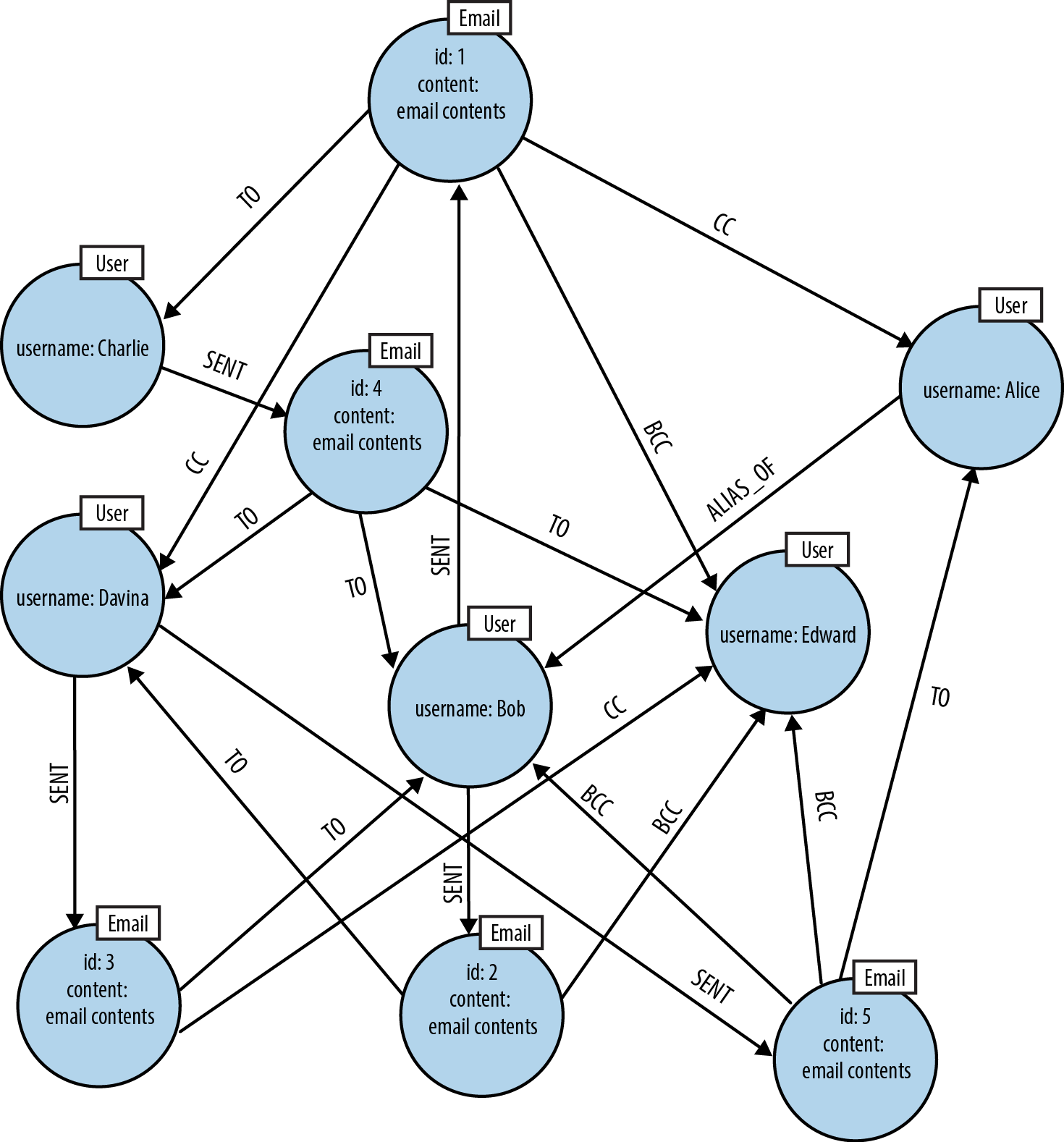
Figure 3-10. A graph of email interactions
We can now query this graph to identify potentially suspect behavior:
MATCH(bob:User {username:'Bob'})-[:SENT]->(email)-[:CC]->(alias),(alias)-[:ALIAS_OF]->(bob)RETURNemail.id
Here we retrieve all the emails that Bob has sent where he’s CC’d one of his own aliases. Any emails that match this pattern are indicative of rogue behavior. And because both Cypher and the underlying graph database have graph affinity, these queries—even over large datasets—run very quickly. This query returns the following results:
+------------------------------------------+
| email                                    |
+------------------------------------------+
| Node[6]{id:"1",content:"email contents"} |
+------------------------------------------+
1 row
Evolving the Domain
As with any database, our graph serves a system that is likely to evolve over time. So what should we do when the graph evolves? How do we know what breaks, or indeed, how do we even tell that something has broken? The fact is, we can’t completely avoid migrations in a graph database: they’re a fact of life, just as with any data store. But in a graph database they’re usually a lot simpler.
In a graph, to add new facts or compositions, we tend to add new nodes and relationships rather than change the model in place. Adding to the graph using new kinds of relationships will not affect any existing queries, and is completely safe. Changing the graph using existing relationship types, and changing the properties (not just the property values) of existing nodes might be safe, but we need to run a representative set of queries to maintain confidence that the graph is still fit for purpose after the structural changes. However, these activities are precisely the same kinds of actions we perform during normal database operation, so in a graph world a migration really is just business as usual.
At this point we have a graph that describes who sent and received emails, as well as the content of the emails themselves. But of course, one of the joys of email is that recipients can forward on or reply to an email they’ve received. This increases interaction and knowledge sharing, but in some cases leaks critical business information. Since we’re looking for suspicious communication patterns, it makes sense for us to also take into account forwarding and replies.
At first glance, there would appear to be no need to use database migrations to update our graph to support our new use case. The simplest additions we can make involve adding FORWARDED and REPLIED_TO relationships to the graph, as shown in Figure 3-11. Doing so won’t affect any preexisting queries because they aren’t coded to recognize the new relationships.
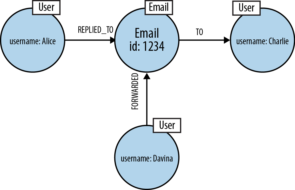
Figure 3-11. A naive, lossy approach fails to appreciate that forwarded and replied-to emails are first-class entities
However, this approach quickly proves inadequate. Adding FORWARDED or REPLIED relationships is naive and lossy in much the same way as our original use of an EMAILED relationship. To illustrate this, consider the following CREATE statements:
...MATCH(email:Email {id:'1234'})CREATE(alice)-[:REPLIED_TO]->(email)CREATE(davina)-[:FORWARDED]->(email)-[:TO]->(charlie)
In the first CREATE statement we’re trying to record the fact that Alice replied to a particular email. The statement makes logical sense when read from left to right, but the sentiment is lossy—we can’t tell whether Alice replied to all the recipients of email or directly to the author. All we know is that some reply was sent. The second statement also reads well from left to right: Davina forwarded email to Charlie. But we already use the TO relationship to indicate that a given email has a TO header identifying the primary recipients. Reusing TO here makes it impossible to tell who was a recipient and who received a forwarded version of an email.
To resolve this problem, we have to consider the fundamentals of the domain. A reply to an email is itself a new Email, but it is also a Reply. In other words, the reply has two roles, which in the graph can be represented by attaching two labels, Email and Reply, to the reply node. Whether the reply is to the original sender, all recipients, or a subset can be easily modeled using the same familiar TO, CC, and BCC relationships, while the original email itself can be referenced via a REPLY_TO relationship. Here’s a revised series of writes resulting from several email actions (again, we’ve omitted the necessary anchoring of nodes):
CREATE(email_6:Email {id:'6', content:'email'}),(bob)-[:SENT]->(email_6),(email_6)-[:TO]->(charlie),(email_6)-[:TO]->(davina);CREATE(reply_1:Email:Reply {id:'7', content:'response'}),(reply_1)-[:REPLY_TO]->(email_6),(davina)-[:SENT]->(reply_1),(reply_1)-[:TO]->(bob),(reply_1)-[:TO]->(charlie);CREATE(reply_2:Email:Reply {id:'8', content:'response'}),(reply_2)-[:REPLY_TO]->(email_6),(bob)-[:SENT]->(reply_2),(reply_2)-[:TO]->(davina),(reply_2)-[:TO]->(charlie),(reply_2)-[:CC]->(alice);CREATE(reply_3:Email:Reply {id:'9', content:'response'}),(reply_3)-[:REPLY_TO]->(reply_1),(charlie)-[:SENT]->(reply_3),(reply_3)-[:TO]->(bob),(reply_3)-[:TO]->(davina);CREATE(reply_4:Email:Reply {id:'10', content:'response'}),(reply_4)-[:REPLY_TO]->(reply_3),(bob)-[:SENT]->(reply_4),(reply_4)-[:TO]->(charlie),(reply_4)-[:TO]->(davina);
This creates the graph in Figure 3-12, which shows numerous replies and replies-to-replies.
Now it is easy to see who replied to Bob’s original email. First, locate the email of interest, then match against all incoming REPLY_TO relationships (there may be multiple replies), and from there match against incoming SENT relationships: this reveals the sender(s). In Cypher this is simple to express. In fact, Cypher makes it easy to look for replies-to-replies-to-replies, and so on to an arbitrary depth (though we limit it to depth four here):
MATCHp=(email:Email {id:'6'})<-[:REPLY_TO*1..4]-(:Reply)<-[:SENT]-(replier)RETURNreplier.usernameASreplier,length(p) - 1ASdepthORDER BYdepth

Figure 3-12. Explicitly modeling replies in high fidelity
Here we capture each matched path, binding it to the identifier p. In the RETURN clause we then calculate the length of the reply-to chain (subtracting 1 for the SENT relationship), and return the replier’s name and the depth at which he or she replied. This query returns the following results:
+-------------------+
| replier   | depth |
+-------------------+
| "Davina"  | 1     |
| "Bob"     | 1     |
| "Charlie" | 2     |
| "Bob"     | 3     |
+-------------------+
4 rows
We see that both Davina and Bob replied directly to Bob’s original email; that Charlie replied to one of the replies; and that Bob then replied to one of the replies to a reply.
It’s a similar pattern for a forwarded email, which can be regarded as a new email that simply happens to contain some of the text of the original email. As with the reply case, we model the new email explicitly. We also reference the original email from the forwarded mail so that we always have detailed and accurate provenance data. The same applies if the forwarded mail is itself forwarded, and so on. For example, if Alice (Bob’s alter ego) emails Bob to try to establish separate concrete identities, and then Bob (wishing to perform some subterfuge) forwards that email on to Charlie, who then forwards it onto Davina, we actually have three emails to consider. Assuming the users (and their aliases) are already in the database, in Cypher we’d write that audit information into the database as follows:
CREATE(email_11:Email {id:'11', content:'email'}),(alice)-[:SENT]->(email_11)-[:TO]->(bob);CREATE(email_12:Email:Forward {id:'12', content:'email'}),(email_12)-[:FORWARD_OF]->(email_11),(bob)-[:SENT]->(email_12)-[:TO]->(charlie);CREATE(email_13:Email:Forward {id:'13', content:'email'}),(email_13)-[:FORWARD_OF]->(email_12),(charlie)-[:SENT]->(email_13)-[:TO]->(davina);
On completion of these writes, our database will contain the subgraph shown in Figure 3-13.
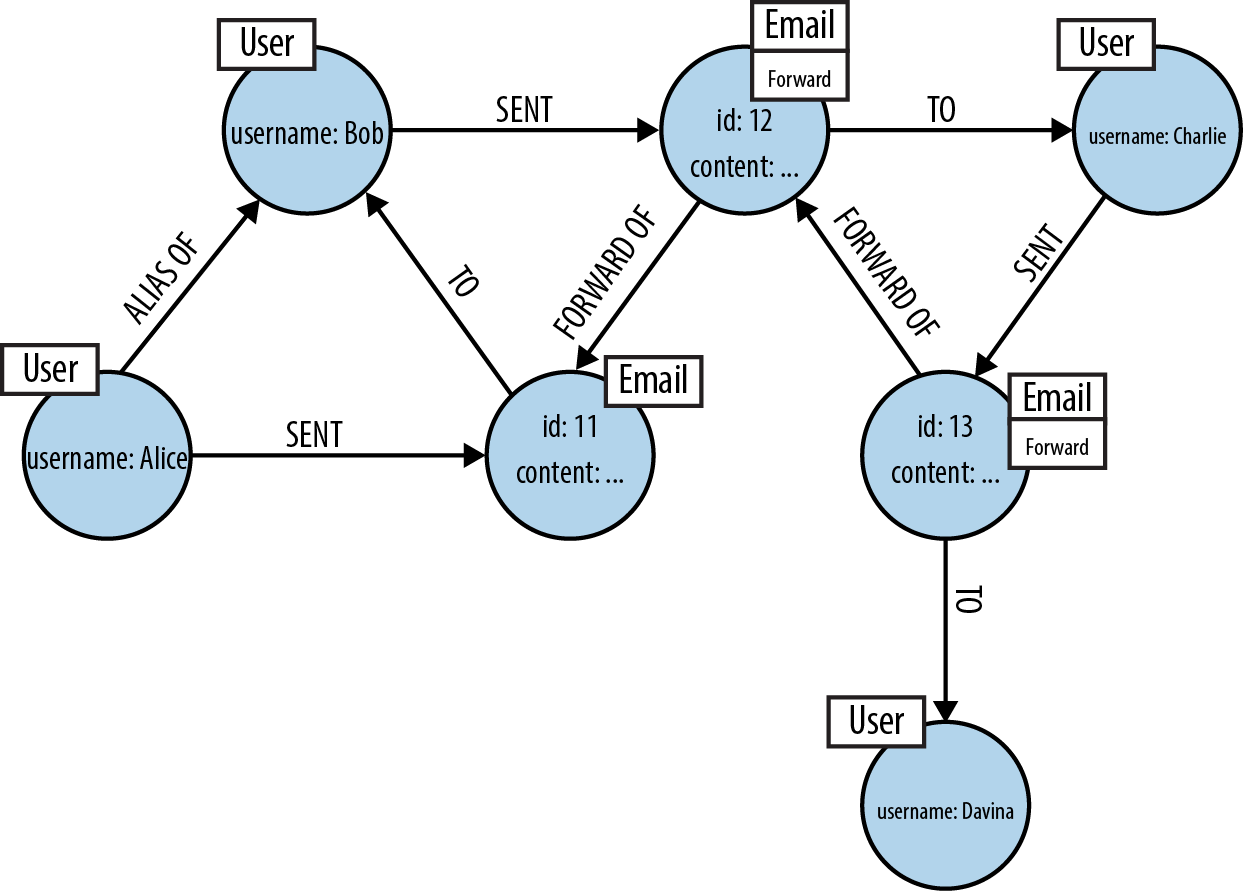
Figure 3-13. Explicitly modeling email forwarding
Using this graph, we can determine the various paths of a forwarded email chain.
MATCH(email:Email {id:'11'})<-[f:FORWARD_OF*]-(:Forward)RETURNcount(f)
This query starts at the given email and then matches against all incoming FORWARD_OF relationships in the tree of forwarded emails to any depth. These relationships are bound to an identifier f. To calculate the number of times the email has been forwarded, we count the number of FORWARD_OF relationships bound to f using Cypher’s count function. In this example, we see the original email has been forwarded twice:
+----------+
| count(f) |
+----------+
| 2        |
+----------+
1 row
Identifying Nodes and Relationships
The modeling process can best be summed up as an attempt to create a graph structure that expresses the questions we want to ask of our domain. That is, design for queryability:
-
Describe the client or end-user goals that motivate our model.
-
Rewrite these goals as questions to ask of our domain.
-
Identify the entities and the relationship that appear in these questions.
-
Translate these entities and relationships into Cypher path expressions.
-
Express the questions we want to ask of our domain as graph patterns using path expressions similar to the ones we used to model the domain.
By examining the language we use to describe our domain, we can very quickly identify the core elements in our graph:
-
Common nouns become labels: “user” and “email,” for example, become the labels
UserandEmail. -
Verbs that take an object become relationship names: “sent” and “wrote,” for example, become
SENTandWROTE. -
A proper noun—a person or company’s name, for example—refers to an instance of a thing, which we model as a node, using one or more properties to capture that thing’s attributes.
Avoiding Anti-Patterns
In the general case, don’t encode entities into relationships. Use relationships to convey semantics about how entities are related, and the quality of those relationships. Domain entities aren’t always immediately visible in speech, so we must think carefully about the nouns we’re actually dealing with. Verbing, the language habit whereby a noun is transformed into a verb, can often hide the presence of a noun and a corresponding domain entity. Technical and business jargon is particularly rife with such neologisms: as we’ve seen, we “email” one another, rather than send an email, “google” for results, rather than search Google.
It’s also important to realize that graphs are a naturally additive structure. It’s quite natural to add facts in terms of domain entities and how they interrelate using new nodes and new relationships, even if it feels like we’re flooding the database with a great deal of data. In general, it’s bad practice to try to conflate data elements at write time to preserve query-time efficiency. If we model in accordance with the questions we want to ask of our data, an accurate representation of the domain will emerge. With this data model in place, we can trust the graph database to perform well at read time.
Note
Graph databases maintain fast query times even when storing vast amounts of data. Learning to trust our graph database is important when learning to structure our graphs without denormalizing them.
Summary
Graph databases give software professionals the power to represent a problem domain using a graph, and then persist and query that graph at runtime. We can use graphs to clearly describe a problem domain; graph databases then allow us to store this representation in a way that maintains high affinity between the domain and the data. Further, graph modeling removes the need to normalize and denormalize data using complex data management code.
Many of us, however, will be new to modeling with graphs. The graphs we create should read well for queries, while avoiding conflating entities and actions—bad practices that can lose useful domain knowledge. Although there are no absolute rights or wrongs to graph modeling, the guidance in this chapter will help you create graph data that can serve your systems’ needs over many iterations, all the while keeping pace with code evolution.
Armed with an understanding of graph data modeling, you may now be considering undertaking a graph database project. In the next chapter we’ll look at what’s involved in planning and delivering a graph database solution.
1 For reference documentation, see http://goo.gl/W7Jh6x and http://goo.gl/ftv8Gx.