
The Flaw of Averages in Cyber Security
Sam Savage, PhD, founder of ProbabilityManagement.org, author of The Flaw of Averages: Why We Underestimate Risk in the Face of Uncertainty, and consulting professor at Stanford. © Copyright 2015, Sam L. Savage.
The “flaw of averages” is a set of systematic errors that occur when uncertain assumptions are replaced with single “average” numbers. The most serious of these, known as Jensen's inequality by mathematicians, states roughly that “plans based on average assumptions are wrong on average.” The essence of cybersecurity is the effective mitigation of uncertain adverse outcomes. I will describe two variants of the flaw of averages in dealing with the uncertainties of a hypothetical botnet threat. I will also show how the emerging discipline of probability management can unambiguously communicate and calculate these uncertainties.
Botnets
A “botnet” is a cyberattack created by malware that penetrates numerous computers, which may then be directed by a command‐and‐control server to form a network that carries out illegal activities. Eventually this server will be identified as a threat, whereupon future communication with it is blocked. Once the dangerous site is discovered, the communications history of the infected computers can pinpoint the first contact with the offending server and yield valuable statistics.
Suppose you have invested in two layers of network security. There is a 60% chance that a botnet virus will be discovered by the first layer, in which case the time to detection averages 20 days, with a distribution as displayed in the left side of Figure B.9. Note that the average may be thought of as the balance point of the graph, marked by ∆. In the remaining 40% of cases the virus is not discovered until the second layer of your security system, in which case the average detection time is 60 days, with distribution shown on the right of Figure B.9.

FIGURE B.9 The distribution of detection times for layers 1 and 2 of a security system
Window of Vulnerability for a Single Botnet
The average overall detection time of this botnet virus may be computed as the weighted average 60% × 20 days + 40% × 60 days = 36 days. So on average we are vulnerable to a single botnet for 36 days. The discipline of probability management1 provides additional insights by explicitly representing the entire distribution as a set of historical or simulated realizations called SIPs.2 Figure B.10 displays the SIPs (in this example, 10,000 simulated outcomes) of both distributions in Figure B.9. Performing calculations with SIPs (SIPmath) can be done in numerous software environments, including the native spreadsheet.

FIGURE B.10 SIPs of 10,000 trials of layer 1 and layer 2 detection times
Recently Microsoft Excel has become powerful enough to process SIPs of thousands of trials using its Data Table function.3 Figure B.11 displays such a SIPmath model that combines the two distributions of Figure B.9 to create a distribution of overall time to detection across both security layers.
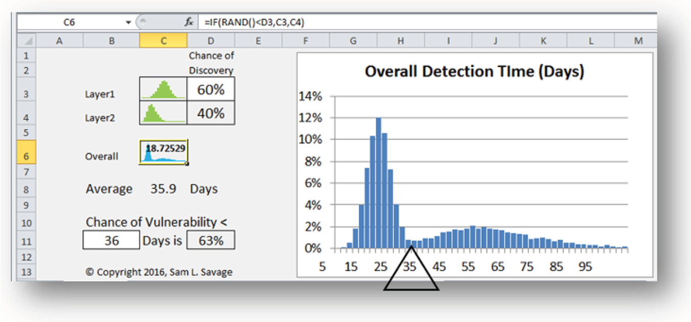
FIGURE B.11 A SIPmath Excel model to calculate the overall detection distribution
This workbook takes the two SIPs of Figure B.10 as input and then performs 10,000 calculations of cell C6 that randomly chooses the layer 1 distribution 60% of the time and the layer 2 SIP 40% of the time. The resulting distribution clearly displays the two modes of detection. Press the calculate key (F9 in Windows, ⌘ = on Mac) to perform a new simulation of 10,000 trials. Note that the simulated average is very close to the theoretical value of 36 days, yet 36 is a very unlikely outcome of the distribution. Also note that because the distribution is asymmetric, the chance of vulnerability of less than the average of 36 days is not 50% but 63%. Experiment with the chance of discovery at layer 1 in cell D3 and the number of days in B11 to see how the distribution, average, and chance change.
The formula used for calculating the average detection time over both layers was technically correct in that it yielded 36 days, but it provides no clue about the distribution. This is what I call the weak form of the flaw of averages. The strong form is considerably worse, in that you don't even get the right average. The model of Figure B.7 created a SIP of its own, which we can now use to explore the impact of multiple simultaneous botnet attacks.
Window of Vulnerability for Multiple Botnets
Suppose we put a new system online, which is immediately attacked by multiple viruses that all have the same distribution of detection times. Since each virus is detected in an average of 36 days, you might think that the average vulnerability is again 36 days, as it was for the single virus. But it is not, because your system remains vulnerable until the last of the botnets is detected.
Figure B.12 displays the SIPs of 10 botnet detection times generated by the simulation of Figure B.11. They all have the same numbers, but the order has been scrambled in each to make them statistically independent.

FIGURE B.12 The detection time SIPs of 10 independent botnets
These SIPs are used in the model in Figure B.13, which calculates the distribution of the maximum of the detection times of all botnets in cell C14. Note that you can adjust the number of botnets from between 1 and 10 with the spinner control in column E. Before experimenting with this model, close the model of Figure B.11, as it contains a Rand() formula, which can slow down the calculation.

FIGURE B.13 Simulation of multiple botnets
Note that the average days of vulnerability increase as the number of simultaneous attacks goes up, and that the chance of coming in at less than 36 days diminishes. This is an example of the strong form of the flaw of averages, and for 10 botnets, the average is 78 days, with a 1% chance of being less than 36.
Such modeling could easily be generalized to reflect different variants of viruses attacking at random times instead of all at once. Such insights into the proportion of time when you would expect your system to be vulnerable are vital to making investment decisions involving mitigation strategies.
Notes
- 1 See Melissa Kirmse and Sam Savage, “Probability Management 2.0,” ORMS Today, October 2014, http://viewer.zmags.com/publication/ad9e976e#/ad9e976e/32.
- 2 SIP stands for stochastic information packet. These arrays of potential outcomes may be generated with a wide variety of readily available simulation software, as well as a native electronic spreadsheet. The cross‐platform SIPmath standard from nonprofit ProbabilityManagement.org allows SIPs to be shared between applications.
- 3 Sam L. Savage, “Distribution Processing and the Arithmetic of Uncertainty,” Savage Analytics Magazine, November/December 2012, http://viewer.zmags.com/publication/90ffcc6b#/90ffcc6b/29.