16
Hysteresis in J–V Characteristics
Wolfgang Tress
Zurich University of Applied Sciences, Institute of Computational Physics, School of Engineering, Wildbachstr. 21, 8401 Winterthur, Switzerland
16.1 Introduction and Definitions: What Do We Mean by Hysteresis?
Several review papers on hysteresis exist already mainly following the same scheme of extensively listing reported results on origins and suggested elimination strategies of hysteresis [1–4]. I myself contributed to a book chapter on this topic recently as well [5]. To create something new, I tried to write this chapter in hand from a different perspective. Instead of reviewing what has been reported, I invite the reader to undertake the journey of exploring and understanding the hysteresis phenomenon in perovskite solar cells (PSCs) by themselves guided by this book chapter.
Prior to jumping into PSCs, which are topic of this book, we want to start with some general points regarding the phenomenon hysteresis. One of the most prominent examples in physics, where we observe hysteresis, is found in the field of magnetism. In a ferromagnetic material, the magnetic flux density B lags behind the magnetization force H, giving rise to a hysteresis loop when B is plotted vs. H. A ferroelectric material behaves analogously, when plotting the displacement field D = ε0E + P(E, …) vs. the electric field E ( ε0 is the vacuum permittivity), where remnant polarization P can be observed (Figure 16.1a). The general scheme behind these effects is a delayed response of the material upon an external force. This leads to remnant effects and therefore a dependence of the measured state on the history of the sample.
Generally speaking we can distinguish two major reasons behind hysteresis:
- A certain threshold force is required to change/switch one quantity such as the magnetic flux density.
- The response time of the material/device is continuously lagging behind while measuring the desired quantity and simultaneously sweeping the relevant force, e.g. the electric field acting on charge carriers by applying a voltage.
The first leads to a rather rate‐independent hysteresis (here labeled as type I) meaning that the hysteresis does not depend on how fast the force is swept but mainly on the history in the sense of previous (extreme) forces, the sample has seen (Figure 16.1a). The second leads to a rate‐dependent hysteresis (type II), meaning that the material or system is not characterized by a single hysteresis. Instead, despite the same scan range of the force, different hysteresis curves exist dependent on the sweep rate. In this case it is essential to state the conditions not only before the measurement, but also during the measurement, i.e. the sweep rate. Ideally, in such a system the hysteresis vanishes when the sweep rate of the force becomes infinitely low.

Figure 16.1 Examples of hysteresis. (a) Hysteresis loop of a ferroelectric material, where displacement field D is plotted vs. electric field E and a remnant polarization Pr is observed, when E = 0. The inset shows a dielectric material, where D = εrε0E. (b) Example of a hysteresis in the current–voltage (JV) curve of a perovskite solar cell measured at a voltage sweep rate of 100 mV/s.
Now we want to move to hysteresis in the current–voltage (JV) curve of electronic devices such as solar cells. In contrast to the aforementioned examples, we would not expect hysteresis in a JV curve because we would implicitly assume that the measured current density J is a unique function of the applied voltage V with the resistance as quotient of both: R = V/(JA) (A is area). Therefore, we would not expect a hysteresis of type I. On the other hand, the JV curve is obtained by sweeping the voltage, which is a dynamic measurement, whose result could depend on the voltage sweep rate, if the response time of the system is low. Usually, we would assume that the voltage sweep is much slower than any electronic process in our system, and we would measure a steady‐state situation, i.e. a unique JV curve. Such a JV curve for a solar cell under standardized illumination and ambient conditions allows us to directly determine the maximum output power of the solar cell by finding the maximum power point (MPP), where the electrical power (density) P = VJ is maximum. Knowing P and the light intensity, we can determine the power‐conversion efficiency (PCE), the main figure of merit of a solar cell. However, if the JV curve unprecedentedly shows hysteresis (Figure 16.1b), we measure two curves, one for scanning the voltage from short circuit to open circuit (called forward scan) and one vice versa (labeled backward or reverse scan). When determining the PCE as just described, this implies two values for the PCE, which is obviously one value too much for a solar cell. After the report of a severe JV hysteresis under common measurement conditions in 2014 [6], a big debate arose on whether reported PCE values for PSCs can be trusted.
To pragmatically resolve this ambiguity in PCE, researchers started to report the hysteresis, i.e. both JV curves, and to calculate an average of the two PCE values. Furthermore, one attempted to quantify the hysteresis with various indices [5, 7], which should provide means of judging the uncertainty of the reported PCE values. However, these attempts neglect the fact that the hysteresis is of type II, i.e. rate‐dependent (will be discussed in detail in Section 16.3), meaning that we do not have only two JV curves (forward and reverse) but a whole set of curves, when we vary the voltage sweep rate. Consequently, the hysteresis index becomes a function of this rate.
As the rate‐dependent hysteresis is indicative of a non‐steady‐state situation at each voltage during the JV measurement, a simple solution to reach more reliable PCE values would be to determine the PCE not from JV sweeps but from a transient measurement of the PCE, where the applied voltage is roughly kept constant. This approach became standard for PSCs [8] and is usually implemented either by:
- – Applying a constant voltage at the MPP determined from a preceding JV sweep and monitoring the transient current, coined “stabilized power output” [6].
- – Dynamically tracking the MPP and monitoring the output power.
In both cases, a convergence of the power is required, whose value is then reported. Usually the measurement is performed for a couple of minutes. This approach re‐established trust in reported PCE values. Furthermore, optimization of the device architecture and, in particular, the contact layers has lead to a reduction of the hysteresis, often making this issue less relevant for determining the PCE of state‐of‐the‐art solar cells.
However, the hysteresis is not completely tamed, and investigations on its origin are still ongoing. Furthermore, it is still unclear to which extent hysteresis and its origins are related to long‐term instabilities of PSCs. Therefore, a profound understanding of the hysteresis is desirable.
The goal of this chapter is to address the hysteresis in a systematic way combining theoretical aspects with experimental evidence on the macro‐ and nanoscale. We will proceed step by step:
- – To understand hysteresis, we need to understand the JV curve of PSCs in general (Section 16.2).
- – To understand the phenomenon hysteresis, we need to characterize the device properly and unravel parameters that govern it (Section 16.3).
- – To propose microscopic origins, we need to develop a consistent picture between theory and experiment (Section 16.4).
In the final section (Section 16.5), we will summarize the current knowledge and address open questions.
16.2 The JV Curve of a Solar Cell: What Does It Tell?
This chapter provides a general brief review on the JV curve of a solar cell, independent of whether there is hysteresis or not. Understanding the factors dominating the JV curve will allow us to better grasp the effects that underlie hysteresis. We want to address
- – The fundamental solar cell structure
- – The photocurrent/short‐circuit current
- – The photovoltage/open‐circuit voltage
- – The ideal JV curve under illumination
- – The ideal JV curve in the dark
- – The voltage dependence of the photocurrent
- – The series and parallel resistance
- – The meaning of the fill factor
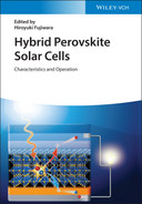
A solar cell is an active device. Under illumination it provides electrical power without any externally applied voltage. This is very different to e.g. a photoresistor as visualized in Figure 16.2. In the convention we are using, power can be generated in the fourth quadrant, where a positive voltage comes along with a negative current. To make such a situation feasible, the photo‐generated electron–hole pairs in our semiconductor absorber have to be spatially separated and collected at two different electrodes. This is only possible if the device exhibits an asymmetric structure. For example, just having one homogeneous photoactive absorber material would not be sufficient to exploit the photoelectric effect in a solar cell, but could work as a photoresistor, a device whose resistance can be modified by light, which changes the charge carrier density (Figure 16.2a). In a solar cell, however, the photo‐generated charges have to flow to their respective electrode without any additional external driving force. This can happen, e.g. in a structure, where an electric field is built into the absorber, such as is the case in a p‐i‐n solar cell. Such a built‐in field can also be caused by a built‐in potential that originates from the work function difference of e.g. the metal contacts. However, such a field is not necessarily required. If electron and hole are able to diffuse efficiently and independently in the absorber, so‐called selective contacts are sufficient to construct a solar cell using a single and homogeneous absorber material (Figure 16.2b). Such selective contacts can be realized by using wide‐gap semiconductors with suitable energy levels to generate a band diagram as depicted in Figure 16.2c.
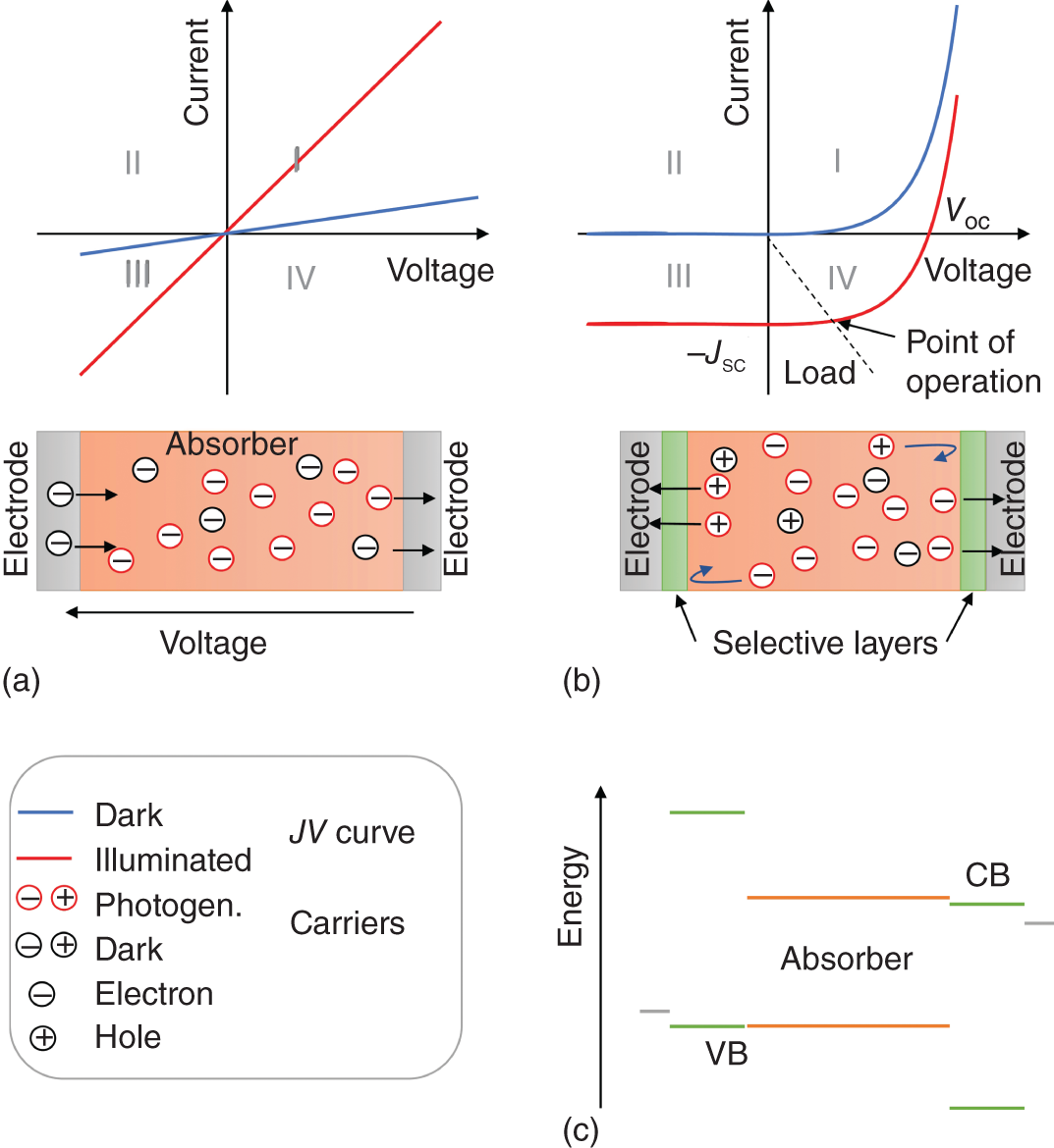
Figure 16.2 Solar cell and photoresistor. (a) Photoresistor as a passive device, where absorption enhances the conductivity by increasing the density of charge carriers (for simplicity, only electrons shown). (b) Solar cell as an active device, being able to provide electrical power in the fourth quadrant, due to a selective collection of electrons and holes at the respective contact. The dashed line shows the negative JV curve of a resistive load. (c) Possible energy diagram of a solar cell with wide‐gap charge‐selective layers. Energy levels (VB, valance band; CB, conduction band, gray work functions of electrodes) are shown vs. a common vacuum level for the individual layers.
Any efficient perovskite solar cell exhibits such selective layers, which are often called electron or hole transporting layer. Despite this name, their major function is actually to block the “other” charge carrier type.
Having realized such a structure, we can examine the photocurrent density under short circuit (Jsc). The short‐circuit current flows when both contacts are connected with a piece of wire, yielding V = 0 V (Figure 16.2b). Jsc is a function of the absorption efficiency and the charge carrier collection efficiency (under short circuit). The former depends on how many photons are absorbed in the absorber material and the latter on how many of these photons are converted into electron–hole pairs that are collected at the electrodes. For optimized PSCs, both quantum efficiencies are rather high. If the collection efficiency is not 100%, photo‐generated charges are lost. The only possible loss process in steady state is recombination of electrons with holes, which brings us to the next point:
The open‐circuit voltage Voc. If we do not connect any load to the solar cell, but just keep the contacts open, we do not extract any electron or hole. Therefore, all photo‐generated charges have to recombine. However, we measure a voltage between the two contacts. Where does this voltage originate from? Coming back to the idea of the previously discussed driving force (drift due to electric field, diffusion due to selectivity), we might imagine that electrons and holes are driven to different electrodes and accumulate there. This accumulated charge might repel further charges and can be measured as an external voltage. This intuitive picture is correct, though a bit simplified and contains the risk of wrong conclusions, such as that the open‐circuit voltage equals the built‐in potential or is limited by it. To be precise, though a bit less intuitive at first glance, we should talk about electrochemical potentials (quasi‐Fermi levels), which we address only very roughly here: Under light we increase both electron (n) and hole (p) densities, as we generate electron–hole pairs (cartoon in Figure 16.2b). Therefore, their chemical potentials rise until a point is reached, where the concentrations are sufficiently high to lead to a recombination rate (R) that is equal to the photo‐generation rate (G) of charge carriers. If we express the recombination rate by R = βnp, which should equal G, we directly see that a higher light intensity (higher G) leads to higher np (β independent of np). Therefore, we can very generally conclude that lower recombination rate constants (here β) lead to higher np for a given G. As the chemical potentials of electrons and holes scale with (the logarithm of) n and p, respectively, the open‐circuit voltage becomes higher for reduced recombination, reaching in the ideal case the thermodynamic limit (around 0.25…0.35 V below the band gap divided by elementary charge, see e.g. in Ref. [9]). Figure 16.3a visualizes how the externally measured voltage relates to the difference of the electrochemical potential of the charge carriers at their respective electrode. Beyond the mentioned radiative recombination R = βnp, recombination at defects and at surfaces/interfaces prevails, which commonly dominates the overall recombination and can lead to gradients in the electrochemical potentials, also under open circuit (Figure 16.3b, details in Refs. [10, 11]). After having understood the concept of recombination and electrochemical potentials, we can now explain the Ideal JV curve under illumination. Short (0 load) and open circuit (infinite load) are extreme cases the solar cell can operate in. Connecting a load with a finite resistance, the solar cell will operate at a current that is between 0 and −Jsc and a voltage that is between 0 and Voc, dependent on the resistance and the J–V relation (JV curve) of the solar cell (dashed line in Figure 16.2b). This JV curve could have various shapes, most intuitively monotonically increasing with voltage, as we were discussing that buildup of the voltage is related to enhanced charge carrier densities, which increase the overall recombination rate and thus decrease the photocurrent. Looking into the (Boltzmann approximated Fermi–Dirac) statistics for charges in their bands, it turns out that there is an exponential relationship between charge carrier densities (and therefore recombination) and the chemical potential (and therefore voltage). This means that when increasing the voltage from 0 to Voc, we enhance the recombination exponentially with voltage, leading to a reduction of the absolute current under illumination and an exponential JV curve (red curve in Figure 16.2b). Having understood this relation between current and voltage, we can also address the question of the JV curve in the dark.

Figure 16.3 Open‐circuit voltage and recombination. (a) Slower recombination leads to higher charge carrier densities and therefore higher voltage V. (b) Visualization of different recombination mechanisms and the fact that optical generation G equals the overall recombination Rrad + RSRH + Rsurf. SRH stands for Shockley–Read–Hall recombination at defects and the arrow bundle indicates generation of heat.
In the dark, there are no photo‐generated carriers, hence no short‐circuit current density or open‐circuit voltage unequal to 0 can be measured. However, if voltage is applied actively by connecting the solar cell to a voltage source, electrochemical potentials move and charge carrier concentrations increase exponentially with voltage, leading to a current that increases exponentially with voltage (blue line in Figure 16.2b), resembling a classical Shockley diode equation:
with ![]() being the thermal voltage and n the ideality factor. The blocking behavior under negative voltage is a direct consequence of the selectivity of the contacts. As this exponential increase in recombination current depends only on the voltage and not on the illumination, we can directly relate the ideal JV curve under illumination with the dark JV curve by just subtracting the Jsc from the dark JV curve, referred to as superposition principle (Figure 16.4a):
being the thermal voltage and n the ideality factor. The blocking behavior under negative voltage is a direct consequence of the selectivity of the contacts. As this exponential increase in recombination current depends only on the voltage and not on the illumination, we can directly relate the ideal JV curve under illumination with the dark JV curve by just subtracting the Jsc from the dark JV curve, referred to as superposition principle (Figure 16.4a):
So far we just discussed that the JV curve is completely defined by recombination current. In a real device, however, the current can be subjected to ohmic losses. In other words, the charge carrier collection efficiency might depend on the voltage, meaning that Jsc in Eq. 16.2 has to be replaced by a photocurrent Jphotothat depends on the voltage:
This can happen if charge carrier diffusivities and mobilities are low. In that case, an electric field originating from the built‐in potential can support charge carrier extraction. As this field is more and more compensated with enhanced voltage, the photocurrent decreases toward open circuit and the curve leaves the ideal diode curve (Figure 16.4b). In extreme cases the curve can show features as depicted in Figure 16.4c and called s‐shape/s‐kink. Such s‐shaped JV curves can also result from non‐optimum properties of the selective contacts. If these contacts are not ideal for the charge carrier to collect, meaning that their conductivity is low or energy levels are misaligned causing charge extraction barriers, photocurrent extraction is strongly hampered in a highly nonlinear way [12, 13]. Piled‐up charges become prone to recombination and only voltages much smaller than Voc can support sufficient extraction of charges.
Apart from these processes related to the absorber and its interfaces, there are further parasitic effects that influence the JV curve, both in the dark and under illumination. Lateral transport through the electrode, wiring, etc. introduce a resistance that is in series to the solar cell (RS). This series resistance does not influence the discussed physics of the solar cell, but modifies the appearance of the externally measured JV curve. For a given current, a certain fraction of the voltage drops over this resistance and the “intrinsic” JV curve could be revealed by correcting the voltage:
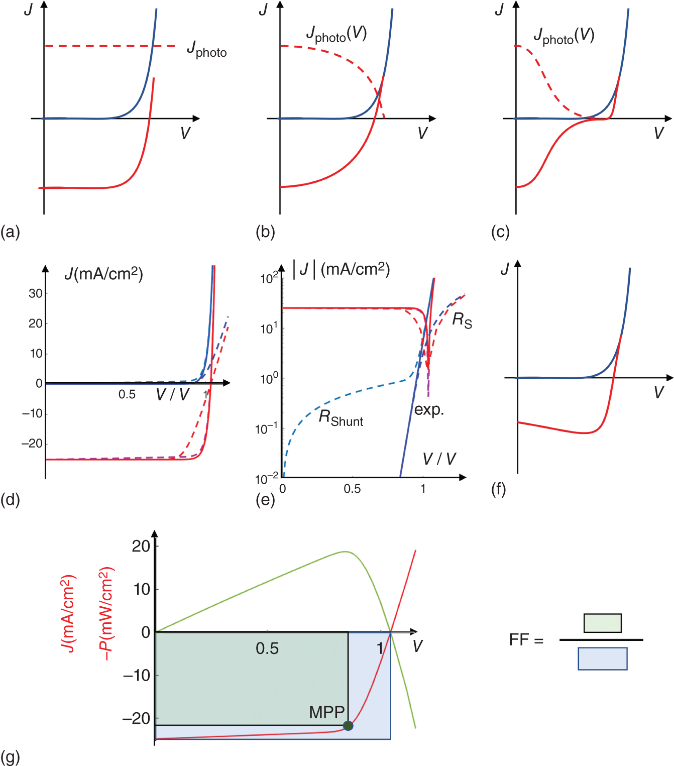
Figure 16.4 The JV curve. (a) Ideal situation with a constant photocurrent Jphoto. (b) Photocurrent that decreases with voltage due to charge collection issues. (c) More extreme case of (b), which causes s‐shape, often due to hindered charge extraction at the contacts. (d) Effect of series resistance (RS = 5 Ω cm2, blue, red dashed) and parallel (shunt) resistance (RShunt = 1 kΩ cm2, cyan, magenta dashed). (e) Data of (d) in logarithmic current scale. (f) “Bump” (g) output power (green) and definition of the FF.
The influence of a series resistance is shown with the dashed red/blue lines in Figure 16.4d,e. Note that it does not modify Voc because current does not flow under open circuit. Leakage currents give rise to a parallel or shunt resistance, often visible close to Jsc and mainly in the dark curve (magenta/cyan dashed lines in Figure 16.4d,e).
All these resistive effects influence the JV curve, including the voltage range between 0 V and Voc. To maximize the PCE, the device should be operated at a current/voltage pair, where the output power P = JV becomes maximum, as stated in Section 16.1. P can be visualized by a rectangular area as shown in Figure 16.4g. The closer this area is to the product of Voc and Jsc, i.e. the more “rectangular” the JV curve, the higher is P. The fill factor (FF) quantifies the ratio of this rectangle to Voc × Jsc. Based on the discussions earlier, we can conclude that a rectangular shape of the JV curve cannot be approached infinitely closely. The closest match is the exponential behavior in the recombination‐limited case with n = 1, which dependent on the Voc can exceed 90% in MAPbI3 solar cells. In experiment FFs lower than the recombination limit are very common due to the discussed charge‐transport limitations and parasitic resistances. In PSCs, it looks like the contact layers with a high selectivity also introduce an obstacle for collecting the desired charge carrier. This limits the fill factor commonly to around 80% for the highly efficient devices.
It is hard to imagine a situation as in Figure 16.4f, where the FF would be even >100%. Such “bump” curves, which are observed for dye sensitized solar cells (DSSC) [14, 15] and PSCs [16], are a clear indication that these curves do not represent a steady‐state situation but must be part of a hysteresis curve.
For more details regarding different recombination mechanisms and correct measurements of PCE and JV curves, the reader is referred to my previous book chapters and reviews [9–11].
16.3 Characteristics of Hysteresis: What Does It Depend on?
Having understood what determines the JV curve in general, we can attempt to investigate the hysteresis. We will approach the phenomenon experimentally step by step without having any predefined hypothesis on its microscopic origin in mind. This is a wise approach for such a complex problem and does not make us mix up cause and effect. It ensures that we will not neglect indirect interactions between charges and electric field in the solar cell stack.
We start with a measured hysteresis curve, shown in Figure 16.1b. Obviously, Voc, Jsc, FF, and hence PCE are lower for the curve obtained from the forward scan. The first question we want to ask is whether the hysteresis depends on the scan rate. We have already anticipated the answer when introducing the two types of hysteresis in Section 16.1. And, indeed, Figure 16.5a confirms a strong rate dependence. For a certain intermediate rate (here around 1000 mV/s), the hysteresis is largest and reduces for lower and higher scan rates. This trend is strong evidence for a process that reacts slowly on the applied bias voltage. If the scan rate is sufficiently low, this process reaches a steady state at each voltage during the scan, and the hysteresis should vanish. If the scan rate is sufficiently high, the slow process cannot react and a quasi‐steady‐state JV curve is measured, which is not unique but depends on the state directly before the measurement (“poling,” preconditioning). This behavior has severe practical consequences:

Figure 16.5 Factors influencing hysteresis. (a) Scan rate for device with more selective contact, where mainly the FF is affected. (b) Scan rate for device with less selective contact (no compact TiO2 layer), where also Voc is affected. (c) Transient response in the dark and (partially) under light. (d) Light‐intensity‐dependent normalized JV curves.
Source: Tress et al. [16].
- – It is not straightforward to make claims on a hysteresis‐free JV curve/device.
- – Even if the hysteresis is negligible at a certain scan rate, it is not guaranteed that the JV curve is a unique steady‐state curve.
- – When comparing two devices at one selected scan rate, a reduced hysteresis does not imply that the origin of the hysteresis got really reduced. It might just be that the rate for the strongest response shifted.
The transient response can nicely be visualized by performing a step‐wise voltage sweep and recording the transients for every voltage step as shown in Figure 16.6a [17, 19, 20].
Although we can already conclude that there is a slow transient process, we leave discussions on its origin for Section 16.4 and proceed with systematically characterizing further parameters.
We continue with the influence of illumination, as the JV curves in Figure 16.5a are measured under illumination. We make use of transient currents again, but this time applying a big voltage step and monitoring the current response. Figure 16.5c shows that it takes a couple of seconds until the current is stabilized. If we repeat the experiment with the device being for part of the time in the dark, it turns out that the response (detectable under light) remains unmodified. Therefore, we can conclude that this slow transient process happens the same way in the dark. To go one step further, we can have a look at the dependence on the light intensity, which can be nicely visualized by plotting normalized JV curves (Figure 16.5d). Also in this case, the hysteresis remains completely independent of light intensity, indicating that the slow process is not directly influenced by absorption of light and/or photo‐generated charge carriers. This observation is consistent with the fact that hysteresis is also observed in dark JV curves. Applying voltages to symmetric devices allows them to develop an asymmetry in their JV curve giving rise to diode characteristics dependent on the sign of the poling voltage [21], which confirms the importance of the applied voltage independent of illumination.
A further important parameter is the temperature [22]. It has been found that it influences the hysteresis in a similar way as the scan rate, meaning that the hysteresis is the highest for a certain temperature and decreases for higher and lower temperatures [23, 24]. Therefore, identical hysteresis curves can be obtained when simultaneously decreasing the temperature and voltage sweep rate, as shown in Figure 16.7b for a photodetector [26]. This is indicative of a temperature‐activated process. At low temperatures, it cannot follow and the hysteresis vanishes, whereas at high temperature it can follow the voltage change completely and the hysteresis vanishes again. For intermediate temperatures, the hysteresis is most pronounced. This temperature dependence of the hysteresis [29] or the transient response [30] has been used to determine an activation energy of the slow process. For devices, which seem to be rather hysteresis‐free for common voltage sweep rates at room temperature, hysteresis can occur at lower temperatures [24, 31].
There is a plethora of metal‐halide perovskite compositions and device architectures. Almost all of these devices show hysteresis to some extent under certain conditions. For example, decreasing the temperature or increasing the scan rate makes a hysteresis appear in devices labeled hysteresis‐free (example of a p‐i‐n device in Figure 16.7c). Therefore, hysteresis is something very prominent in PSCs. However, e.g. in p‐i‐n small‐molecule organic solar cells based on zinc phthalocyanine:C60, hysteresis could not be detected for common scan rates (<100 V/s) (Figure 16.7d).

Figure 16.6 Non‐capacitive and capacitive effects. (a) Transient current response (blue) during a staircase voltage sweep (green), revealing an initially higher charge collection efficiency after increasing the voltage, which looks similar to a classical capacitive response, where the displaced charge would be gigantic (mC/cm2).
Source: (a) Christoforo et al. [17]. Licensed under CC BY 4.0. (b, c) Capacitive dark currents in the order of 10…100 nA/cm2. Jcap in (c) is obtained from J in (b) by subtracting the approximate steady‐state current.
Source: (b) Almora et al. [18].
Nevertheless, already in the early days it has been observed that hysteresis can be tuned by the solar cell architecture, the adjacent charge transport layers, and also the perovskite itself. A common trend seems to be that hysteresis decreases when changing the electron transport layer from planar TiO2 to planar SnO2 or mesoporous TiO2 [20, 32]. Modifications of the oxide contacts using e.g. phenyl‐C61‐butyric acid methyl ester (PCBM) reduce hysteresis as well [33, 34]. Modifications or elimination of the p‐side contact seems to influence the hysteresis less according to my experience but exchanging spiro‐MeOTAD by CuI leads to reduced hysteresis [35]. When flipping the layer sequence (from n‐i‐p to p‐i‐n) and using organic contact layers, the hysteresis vanishes at common scan rates [36–38]. However, also in this architecture hysteresis can be prominent, e.g. when a NiOx hole transport layer is used or at higher scan rates (Figure 16.7c). Also in the inverted structure, PCBM in between perovskite and C60 has turned out to be beneficial in reducing hysteresis [39].
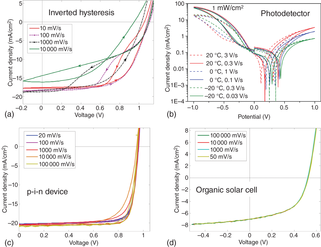
Figure 16.7 Hysteresis in different solar cells. (a) Inverted hysteresis, as e.g. observed at instable mixed perovskites.
Source: Adapted from Tress et al. [25]. Copyright 2016 WILEY‐VCH Verlag GmbH & Co. KGaA, Weinheim. (b) Temperature and rate dependence of hysteresis of a photodetector.
Source: Adapted from Domanski et al. [26]. Copyright 2015 WILEY‐VCH Verlag GmbH & Co. KGaA, Weinheim. (c) Planar p‐i‐n device with architecture presented in Ref. [27].
Source: Based on Chiang et al. [27]. (d) Organic solar cell ZnPc:C60 with structure shown in Ref. [28].
Source: Based on Tress et al. [28].
Having a look at the perovskite layer itself, also some trends have been observed: For n‐i‐p devices with a mesoporous TiO2 electrode, the hysteresis becomes more prominent with reduced grain size [20, 40]. In this case, the increased hysteresis is accompanied by a reduced FF. On the other hand, PSCs that are vacuum‐deposited are almost hysteresis‐free independent of architecture despite small grains in the film [41]. The composition of the perovskite itself independent of the morphology might be relevant and materials present at grain boundaries such as PbI2 seem to influence hysteresis as well [42, 43]. In addition, additives can modify the hysteresis, where e.g. PCBM [44], carbon nanoparticles [45], or potassium iodide [46] have been found to reduce hysteresis.
The JV hystereses in the figures presented so far have one feature in common despite the different shape and differently affecting Jsc, FF, and Voc: The reverse scan yields higher PCE values than the forward scan. However, this feature is not to be generalized and there are devices that show the opposite behavior, also called inverted hysteresis (Figure 16.7a) [25]. It is even possible that the same device can change from normal to inverted hysteresis upon light soaking or dependent on the scan rate. Furthermore, the JV curves from forward and reverse scan can cross (several times) between 0 V and Voc.
From the phenomenological characterization of hysteresis and experimental variation of the contact and absorber layers in PSCs, we can conclude:
- – Hysteresis in PSCs is universal but not unique: It depends on measurement conditions (scan rate, temperature, preconditioning). Therefore, it is ambiguous to talk about “hysteresis‐less” devices, when comparing only two JV curves.
- – Hysteresis is triggered by changes in voltage due to a slow transient process in the PSC. It is most pronounced when scan rate and the dynamics of this slow process are on the same timescale.
- – Factors in the device design influencing the appearance of hysteresis are various: A single culprit or a magic modification that universally removes hysteresis cannot be identified.
- – Properties of the contact layers have the strongest influence on hysteresis.
- – Hysteresis occurring on slow timescales of minutes can lead to a smooth transition to reversible [47] and irreversible degradation phenomena.
In Section 16.4 we want to finally address possible reasons for such a slow response and identify the most likely one that consistently describes the experimental data.
16.4 Mechanistic and Microscopic Origin of Hysteresis: What Changes Slowly?
In this section, we want to go the reverse way compared with Section 16.3. We start with hypotheses based on microscopic theories and scrutinize whether they can describe the “slow process” and its consequences.
We start with capacitive effects. As we are performing a voltage sweep, we are applying a continuously changing voltage, characterized by the sweep rate dV/dt. The changing electric field results in a displacement current ![]() , which can be expressed as a capacitive current:
, which can be expressed as a capacitive current:
Such a capacitive current occurs in the dark and under illumination. To judge whether it plays a role in the hysteresis, we calculate this current assuming a realistic “geometric” capacitance of 50 nF/cm2 (plate capacitor model: ![]() with thickness d = 500 nm and εr ≈ 30). We make the case more realistic by considering a finite resistance that the current faces when charging the capacitor (R = 100 Ω cm2, unrealistically high for a series Rs/A in Eq. 16.4).
with thickness d = 500 nm and εr ≈ 30). We make the case more realistic by considering a finite resistance that the current faces when charging the capacitor (R = 100 Ω cm2, unrealistically high for a series Rs/A in Eq. 16.4).
Figure 16.8a shows the results with the following characteristic features: As obvious from Eq. 16.5, the capacitive current is independent of voltage for a constant scan rate ![]() and proportional to the scan rate, changing sign with the sign of the sweep rate. The current‐limiting effect of R is visible when modifying the sweep rate. Comparing these data with the hysteresis in Figure 16.5, we observe that the features look different and that the values of C required for the current to show up in the hysteresis plot (e.g. several mA/cm2 at 100 mV/s) would be gigantic (Figure 16.8b shows a case for 1 V/s and 1000 × larger capacitance). Therefore, we can already conclude that the type of hysteresis seen in Figure 16.5 is not caused by capacitive effects. Nevertheless, also capacitive effects can be observed in PSCs, e.g. in μs transients [48], when using high scan rates, or when investigating dark currents, where the steady‐state currents around 0 V are much lower than under solar illumination. This is e.g. shown in Figure 16.6b,c from Ref. [18]. Note that the currents have similar positive and negative values in the order of 10–100 nA/cm2, compatible with a capacitance value of 3 μF/cm2. This value is realistic for an accumulation capacitance of e.g. ionic charges at the interface between charge transport layers and perovskite. Figure 16.8c shows that such capacitive effects are expected to become visible in the JV curve under solar illumination for scan rates in the kV/s range. Capacitive effects have been observed in other solar cell technologies as well, e.g. in Si [49] or CdTe [50].
and proportional to the scan rate, changing sign with the sign of the sweep rate. The current‐limiting effect of R is visible when modifying the sweep rate. Comparing these data with the hysteresis in Figure 16.5, we observe that the features look different and that the values of C required for the current to show up in the hysteresis plot (e.g. several mA/cm2 at 100 mV/s) would be gigantic (Figure 16.8b shows a case for 1 V/s and 1000 × larger capacitance). Therefore, we can already conclude that the type of hysteresis seen in Figure 16.5 is not caused by capacitive effects. Nevertheless, also capacitive effects can be observed in PSCs, e.g. in μs transients [48], when using high scan rates, or when investigating dark currents, where the steady‐state currents around 0 V are much lower than under solar illumination. This is e.g. shown in Figure 16.6b,c from Ref. [18]. Note that the currents have similar positive and negative values in the order of 10–100 nA/cm2, compatible with a capacitance value of 3 μF/cm2. This value is realistic for an accumulation capacitance of e.g. ionic charges at the interface between charge transport layers and perovskite. Figure 16.8c shows that such capacitive effects are expected to become visible in the JV curve under solar illumination for scan rates in the kV/s range. Capacitive effects have been observed in other solar cell technologies as well, e.g. in Si [49] or CdTe [50].
In addition to this textbook‐like displacement current, further capacitive/charge accumulation effects might be considered to explain the hysteresis. Those are related to storage of electrons or holes as a function of prebias and their collection as a function of sweep rate. Such an effect was proposed to explain the already mentioned “bump” in the JV curve [51]. However, absence of the bump in the dark and the peak current under light always being smaller than the maximum obtainable photocurrent in the PSCs do not advocate for such an effect.
Naturally, the hysteresis comes along with “capacitive” effects seen in impedance spectroscopy, yielding results of gigantic and photoinduced capacitances [52, 53]. However, these results are unphysical when interpreted literally. They cannot be taken as a support of capacitive currents because they are just a manifestation of the same slow process in another measurement. Therefore, these capacitances have to be seen as apparent capacitances, not directly originating from charge stored somewhere in the device [54–57].
This brings us to non‐capacitive origins of hysteresis, which are the dominating ones for the common hysteresis observed at low scan rates (V/s to mV/s) and under light [16, 19, 58, 59]. (Most of the effects assigned to capacitive contributions in Ref. [60] are assigned to the non‐capacitive category in this book chapter.)
The already mentioned poling effects on symmetrical devices, which become p–n or n–p diodes dependent on prebias [21], are strong evidence that electrical properties can be modified by applying a voltage and remain for a certain time. A direct proof of slowly changing electric fields upon a voltage step was obtained by Kelvin probe force microscopy (KPFM) measurements on cross sections of solar cells (Figure 16.9) [61].
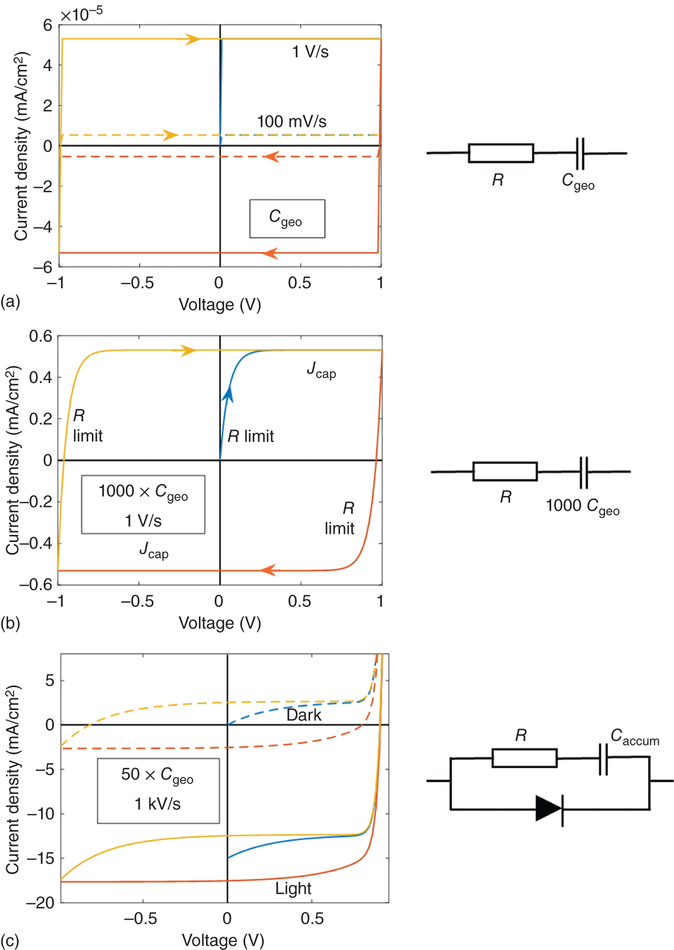
Figure 16.8 Demonstration of capacitive effects. (a) Calculated current vs. voltage for forward and backward scan with typical scan rates considering the geometric capacitance. (b) 1000 × higher capacitance and 1 V/s scan rate to reach about Jcap ≈ 1 mA/cm2. (c) Capacitive effects superimposed on diode JV curves. The photocurrent is 15 mA/cm2. R is 100 Ω cm2 and the scan rate 1 kV/s.
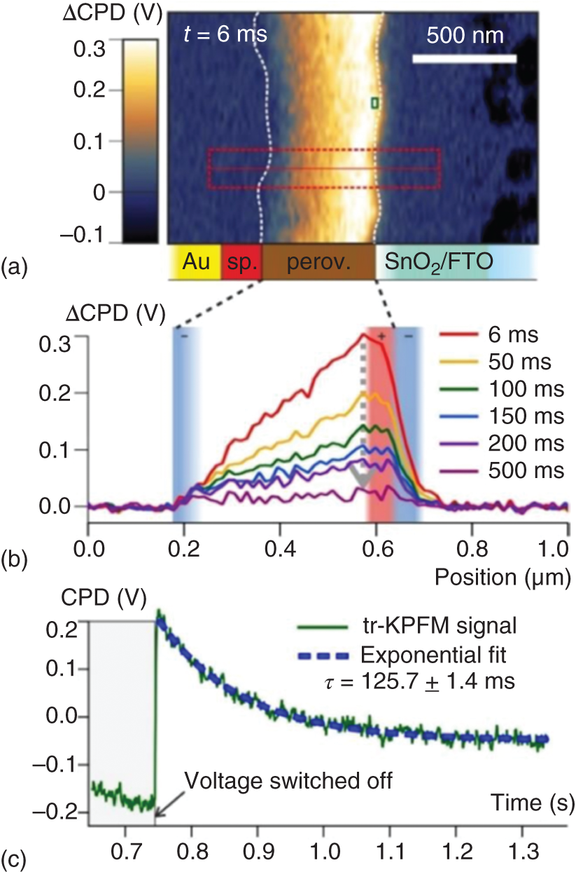
Figure 16.9 Transient KPFM measurements of perovskite solar cells upon switching the applied voltage from 0.5 to 0 V. (a) Contact potential map 6 ms after switching the voltage. (b) Evolution of the potential with time. (c) Contact potential transient at the SnO2 interface.
Source: From Weber et al. [61]. Published by The Royal Society of Chemistry.
Recalling the theory on the JV curve in Section 16.2, we understand that the hysteresis has to be a result of modified charge carrier collection and recombination dependent on the history (prebias and scan rate) of the device (Jphoto(V) in Eq. 16.3 becomes Jphoto[V, scan rate, prebias]). In other words, the hysteresis (and the associated giant capacitance) appears when probed by electron–hole currents, in particular under illumination, whereas the underlying microscopic mechanism governs the timescale and less the magnitude of the effect.
Already in the first paper [6] dedicated to the JV hysteresis, three origins for the remnant electric field in the perovskite have been proposed:
- Purely electronic origin due to
- Deep electronic traps: Charges trapped predominantly at interfaces would cause remnant space charge and affect the JV curve. So far, no clear evidence has been collected for this hypothesis.
- Electron/hole transport: Sometimes insufficient charge collection due to imbalanced electron/hole transport is discussed as reason for the hysteresis [37, 62, 63]. As electron/hole dynamics happen on much faster timescales, we exclude this effect as the underlying mechanism.
- Ferroelectrics, meaning that an electric polarization remains after switching off the electric field (cf. Figure 16.1a); or in other words, the existence of a spontaneous polarization that can be switched by an external electric field: Perovskites can be ferroelectric, either by displacement of lattice sites leading to a polar distortion [64] or by oriented dipolar cations such as MA [65]. For MAPbI3, the latter is unlikely due to a ps scale randomization of the MA orientation [29, 66]. Regarding the former, the absence of a (detectable) second harmonic signal was taken as an indication for a centrosymmetric, nonpolar structure of all phases in a recent study [67]. Later, second harmonic generation has been reported for tetragonal MAPbI3 [68].
The fact that hysteresis can be as prominent in Cs or FA‐based perovskites shows that the orientation of MA can be excluded as a major reason. Here, we leave the discussions on the existence of ferroelectric domains at room temperature to the experts. Some identified them [69] related to tetragonal‐to‐cubic phase transitions [70, 71], others exclude their existence, despite theoretical predictions [72] or mainly by alternative interpretations of the microscopic measurements [73–75]. Some studies clearly rule out a ferroelectric origin of the hysteresis [76]. Here, we just conclude that we cannot see clear indications that ferroelectric domains influence the JV curve or are even required to explain efficient charge separation and transport in metal‐halide perovskites as hypothesized in Refs. [77–80]. Only for completely unrealistically high recombination rate constants, ferroelectric polarization was shown to influence the FF in a simulation study [81].
- Mobile ions: Metal halide perovskites are ionic conductors [82–84], meaning that defect ions such as halide vacancies are mobile and tend to accumulate at the surface of the perovskite to screen the electric field [85], which confirms the intuitive pictures brought up for hysteresis [16]. The double layer formed can be seen in the capacitance under low voltage and in the dark. Ion diffusion has been identified in a Warburg feature [86] or by transient capacitance measurements [87] yielding diffusion coefficients in a range of 10−12–10−8 cm2/s. Theoretical work in combination with temperature‐dependent experiments revealing activation energies for mobile ions provides strong evidence for halide vacancy migration being the response‐time‐determining process [29, 30, 88], although the error bars and parasitic influences on experimentally determined activations energies hardly allow for a meaningful comparison [89]. The picture of mobile ions being the source of changed charge‐carrier collection and recombination probabilities is well supported and developed by numerical device simulation [90–94] that is capable of reproducing the major features of hysteresis.
There are several studies explicitly comparing ferroelectric and ionic origins of hysteresis, concluding that the ionic origin is the more likely one [76, 95].
Now we examine whether and how mobile ions allow for a consistent explanation of aforementioned experimental observations. The basic concept is sketched in Figure 16.10, indicating that for each applied voltage, mobile ions equilibrate in a way to reduce/minimize the electric field in the perovskite (situation at short circuit shown assuming an electric built‐in potential). Consequently, when sweeping or switching to a lower voltage (“backward”), the generated electric field is beneficial for drift‐assisted charge collection. When switching or sweeping to a higher voltage (“forward”), as shown in the right panels of Figure 16.10, the electric field opposes charge collection at the designated electrodes. Once the ions have equilibrated, this effect diminishes and the current stabilizes, as seen in the transients in Figure 16.6. We discuss along the following list whether this explanation is fully consistent with experimental observations:
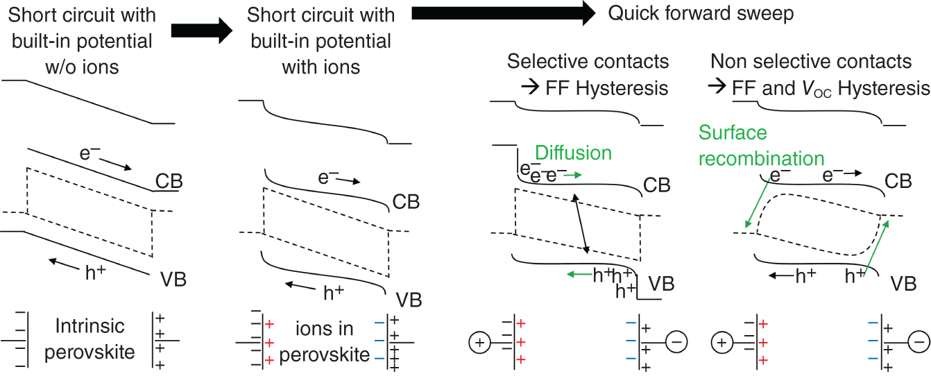
Figure 16.10 Band diagrams showing the flow of photo‐generated electrons and holes in their respective bands. Mobile ions partially screen the electric field in the perovskite by accumulating at interfaces. A forward sweep in voltage faster than the response time of the ions leads to an unfavorable electric field for charge extraction. Dependent on the selectivity of the contacts, not only FF but Voc is affected as well (compare with Figure 16.5a,b).
Source: Tress [89].
- – Rate dependence of hysteresis (Figure 16.5a): Yes, hysteresis when measured in a JV loop becomes largest, when the response time (i.e. transit time according to the sketches in Figure 16.10) is in the time range the JV scan takes. For slower scans, ions can follow and hysteresis reduces; for much faster scans, ions cannot follow and hysteresis reduces as well. If forward and backward curves are not measured in a loop but after equilibration at the starting voltage, hysteresis would not vanish at higher scan rates.
- – Temperature dependence (Figure 16.7b): Yes, it is analogous to the scan rate. Lower temperatures decrease ion mobility and hysteresis might become more or less apparent dependent on the scan rate. A simultaneous reduction of temperature and scan rate can lead to the same hysteresis (Figure 16.7b). In other words, when decreasing the temperature, the scan rate, where hysteresis is maximum, becomes lower [26].
- – Light‐intensity independence (Figure 16.5c,d): Yes, because the ion distributions are mainly influenced by the voltage and the effect on the relative charge collection efficiency is independent of illumination intensity. If the ionic conductivity depends on illumination as discussed in Ref. [85] and found in Ref. [96], the hysteresis might change. How pronounced this change is expected to be should be clarified by device simulation.
- – Lower FF in forward scan (Figure 16.5a): Yes, it fits the idea that the ions screen the electric field and a forward scan, where voltage is applied that opposes charge collection, leads to a lower FF (Figure 16.10).
- – Lower Voc in forward scan (Figure 16.5b): Yes. In this case, it is not sufficient to only discuss modified charge collection, but also changed recombination probabilities. The most straightforward example is surface recombination, where charges are lost at the wrong electrode (cf. Figure 16.3b). Ion distributions caused by a positive prebias induce an electric field that increases the selectivity of the device, whereas ions equilibrated at low or negative voltage decrease the selectivity (Figure 16.10 right panel).
- – Modified forward (dark) currents: Yes, ions accumulated at interfaces to charge transport layers together with electronic counter charge on the electrodes, create interface dipoles, which modify charge injection properties. The lower or even negative the prebias, the more positive (negative) is the ion concentration at the hole (electron)‐injecting contact, hindering forward current.
- – Grain size and composition dependence: This is a complex problem and trends are not unique (cf. Section 16.3). Theoretical descriptions of ion motion are commonly limited to single crystals. Whether grain boundaries impede ion migration or whether ion migration is facilitated by grain boundaries remains an open question. Furthermore, grain boundaries affect electron/hole transport as well [40]. Thus, it is not surprising that the hysteresis is influenced by the morphology albeit predictions are not possible.
- – Inverted hysteresis (Figure 16.7a): Yes, more complex shapes of hysteresis can be explained. It was proposed that in case of inverted hysteresis, charge extraction at the contacts is the bottleneck due to extraction barriers [25] or reversed band bending [97]. In such a case, lower prebias is beneficial as accumulated ions improve charge extraction by the enhanced electric field close to the contact(s).
- – Timescale and quantities: So far we have been talking about a “slow” process without clearly specifying the timescale. And we have been discussing migrating ions without talking about their concentrations. We analyze these parameters with Table 16.1, which shows that a broad range of diffusion coefficients and ion concentrations are reported. We can conclude that from various transient measurements, also on non‐solar‐cell architectures, a mobile ionic species with a diffusion coefficient in the range of 10−9–10−8 cm2/s has been identified and attributed to iodine vacancies [84]. Such a diffusion coefficient would result in hysteresis at scan rates in the order of 100 V/s, where capacitive and non‐capacitive contributions are relevant as shown by Neukom et al. [101], who simulated not only the JV hysteresis but also a set of complementary experiments. This hysteresis, which also becomes apparent for nominally “hysteresis‐free” devices, is consistent with the idea that the underlying mechanism is ion migration in the perovskite. However, to reproduce the common hysteresis at scan rates in the mV/s regime using device simulations, the ion mobility has to be decreased by 3–4 orders of magnitude. Furthermore, the ion densities are set in the order of 1018–1019 cm−3 to provide sufficient space charge to screen the electric field and show influence on the charge collection efficiency. Measured values, however, are more in the 1016–1017 cm−3 regime. One explanation would be that ions in “hysteresis‐devices” are much slower as proposed by Bertoluzzi et al. [99]. However, this is unlikely as also in these devices the “fast” contribution can be seen, e.g. in impedance spectroscopy. Another explanation would be that there is an additional slower mobile ionic species, as e.g. observed in Futscher et al. [87], where, however, the charge of the fast species is negative, which is in contradiction to the consensus that it should be a halide vacancy (positive). Furthermore, the explanation of a slower species is problematic as the slower species should be present also in hysteresis‐less devices. Nevertheless, the simulations are capable of reproducing the hysteresis in the mV/s range very well, as long as slow mobile ions are assumed. As these simulations describe the effect of this slow process, not the dynamics itself, we would conclude that compared with hysteresis‐less devices, either the electric field in the perovskite is much lower than predicted from these simulations, as it e.g. drops on a low‐mobility transport layer, or the mobility of the ionic charge is strongly reduced, e.g. because these ions get stuck at interfaces.
- – Interface dependence: An obvious question is why do we extensively discuss mobile ions in the perovskite as underlying reason for the hysteresis, knowing that p‐i‐n devices with organic charge transport layers hardly show hysteresis? One can counter this question by saying that hysteresis in oxide‐based n‐i‐p devices can be widely tuned by the perovskite composition itself without modifying the contacts. The proper answer to this apparent paradox is that hysteresis is a product of an interplay between ion motion, setting the timescale, and the “reaction” of electronic charges, expressing the result in the JV curve. That is why it is not astonishing that certain electronic and ionic properties need to be fulfilled when simulating the hysteresis with numerical device simulators, such as existence of mobile ions and surface traps [90]/surface recombination [93] or mobile ions paired with extraction barriers [104] if recombination is not sufficiently strong. This interplay is summarized in Figure 16.11 from Ref. [89]. The consequence is that there are many handles to tune hysteresis, both on the ionic and electronic material and device properties. Nevertheless, this interplay cannot explain the different timescales, where halide vacancy migration is expected to happen compared with the ion mobilities required to reproduce hysteresis (cf. Table 16.1). This discrepancy could indeed be due to the influence of the charge transport layers. Recent device simulations have examined the role of charge transport layers and found that their properties indeed affect hysteresis. It was reported that the timescale decreases slightly with the product of doping concentration and dielectric constant [103], however, not to an extent to describe the difference between TiO2 and p‐i‐n devices. Another simulation study showed that energetic barriers at the interface to the electron transport layer tune the appearance of hysteresis without modifying ionic parameters [104]. This is another example, demonstrating the importance of the electronic–ionic interplay sketched in Figure 16.11 and its subtle nuances that are yet to be discovered.
Table 16.1 Parameters for mobile ions in MAPbI3, deduced by various experimental and simulation approaches.
| Method | Scan ratea) | Diffusion coefficient (cm2/s) | Mobility at 300 K (cm2/(V s)) | Concentration (cm−3) | Mobile speciesb) | References | |
|---|---|---|---|---|---|---|---|
| Transient current, dark | 2.4 × 10⁻⁸ | 9.3 × 10⁻⁷ | 5 × 10¹⁶c) | I− (measured) | Yang et al. [84] | Measurement | |
| Electrochemical impedance spectroscopy (EIS), Warburg fit light only | 1.4 × 10⁻¹² | 5.4 × 10⁻¹¹ | MA+ | Bag et al. [86] | |||
| Transient capacitance | 3 × 10⁻⁹ | 1 × 10¹⁵ | I− | Futscher et al. [87] | |||
| 3 × 10⁻¹² | 1.3 × 10¹⁶ | MA+ tetragonal grain boundary (GB) | |||||
| 7 × 10⁻¹² | 1.3 × 10¹⁶ | MA+ cubic GB | |||||
| 2 × 10⁻¹² | 5 × 10¹⁵ | MA+ cubic | |||||
| Photoluminescence (PL) migration | 1 × 10⁻⁹ | 5 × 10⁻⁸ | I− | Li et al. [98] | |||
| Transientsd) | 8 × 10⁻⁹ | 3 × 10⁻⁷ | 1 × 10¹⁸ | Bertoluzzi et al. [99] | |||
| Charge upon voltage step | 4 × 10¹⁷ | Bertoluzzi et al. [100] | |||||
| DD simulated transients + hysteresis | 100 V/s | 1 × 10⁻⁹/3 × 10−16 | 5 × 10⁻⁸/1 × 10−14 | 5 × 10¹⁷/5 × 1017 | Cation/anion | Neukom et al. [101] | Fitting simulated |
| DD simulated | 100 kV/s | 2 × 10⁻⁶ | 1 × 10⁻⁴ | 1 × 10¹⁸ | van Reenen et al. [90] | ||
| Estimated | 1 V/s | 2 × 10⁻¹¹ | 1 × 10⁻⁹ | ||||
| DD hysteresis fit | 1 V/s 250 mV/s | 1 × 10⁻¹¹ 3.7 × 10⁻¹² | 5 × 10⁻¹⁰ 1.4 × 10⁻¹⁰ | 1.6 × 10¹⁹ | Cation | Richardson et al. [91] | hysteresis to experiment |
| DD fit to transients dark current | 7.5 × 10⁻¹³ | 3 × 10⁻¹¹ | 1.6 × 10¹⁹ | Cation | O'Kane et al. [102] | ||
| DD hysteresis fit | 40 mV/s | 1 × 10⁻¹² | 5 × 10⁻¹¹ | 1 × 10¹⁹ | Cation | Calado et al. [93] | |
| Only DD simulated, parameters from prev. publ. | 75 mV/s | 1 × 10⁻¹³ | 5 × 10⁻¹² | 1.6 × 10¹⁹ | Cation | Courtier et al. [103] | |
| Only DD simulated, parameters from prev. publ. | 20 mV/s | 1 × 10⁻¹³/1 × 10−13 | 5 × 10⁻¹²/5 × 10−12 | 1 × 10¹⁸/1 × 1018 | Anion/cation | Sun et al. [104] | |
| Only DD simulated, parameters from prev. publ. | 240 mV/s | 2 × 10⁻¹² | 1 × 10⁻¹⁰ | 5 × 10¹⁷ | Yang et al. [105] |
DD stands for drift‐diffusion device simulation.
a) Order of magnitude, where hysteresis is pronounced.
b) Commonly assigned with reference to preceding literature such as density functional theory (DFT) calculations.
c) Deduced from the published conductivity value.
d) Mixed perovskite composition.
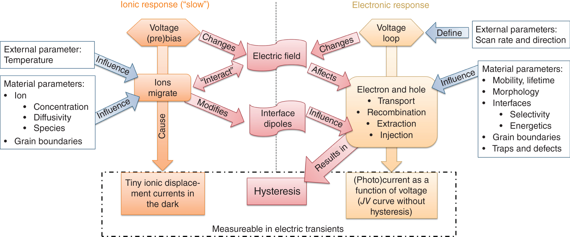
Figure 16.11 Interplay of ionic and electronic response focusing on the electrostatic effect of the mobile ions. The JV hysteresis seen in Figures 16.1b and 16.5 is a result of slowly modified electron/hole currents.
Source: Tress [89].
16.5 Issues with Hysteresis: How to Tune/Avoid/Suppress?
The brief literature overview in Section 16.3 showed that many factors influence hysteresis. In Section 16.5, we saw that this is not surprising as many properties of the material and the device stack influence the “outcome” of the mixed ionic electronic conductivity. Therefore, it is not astonishing that the literature does not offer a conclusive strategy to suppress hysteresis. Based on earlier explanations, we can conclude the following: Measures that are beneficial for the PCE are the best candidates for decreasing hysteresis as well [92], because
- – “Passivation” measures reduce recombination losses at interfaces to the contact layers and hence increase contact selective. This makes the device less prone to surface recombination and thus less sensitive to changes in the electrostatics by mobile ions.
- – “Good” morphology, i.e. films with low defect densities and high overall charge carrier mobilities, allows for a solar cell, working efficiently in a diffusion‐driven regime. Thus, charge collection does not rely on the electric field and its modification by moving ions.
- – Conductive charge transport layers minimize voltage losses during current flow and avoid accumulation of electronic charge. Therefore, efficient charge extraction does not rely on an electric field, which could be compromised by mobile ions.
Measures targeting directly the mobile ions by decreasing their mobility or density are less straightforward, as it is expected that they would mainly shift the timescale where hysteresis is observable. Furthermore, as the ions are intrinsic defects, their equilibrium concentration is given by thermodynamics, and a certain concentration is therefore unavoidable. Due to their low formation energies and a potential dependence on illumination, they are dynamically generated and eliminated [106]. Extrinsic ions such as Li (dopant of the hole‐transport material spiro‐MeOTAD) have been reported to contribute to hysteresis as well [107]. Therefore, their trajectories should be controlled, also with respect to the long‐term device stability.
16.6 Conclusion and Open Questions
Hysteresis in the JV curve of PSCs is a rather universal feature that is mostly of non‐capacitive origin. Instead, collection and extraction efficiencies of photo‐generated charge carriers and thus the fraction of recombining charges become a function of the history, i.e. prebias and voltage sweep rate. Hysteresis is more pronounced the more important an electric field is for charge extraction, such as for low‐conductivity active and charge transport layers. The microscopic process causing this delayed response of the electric field are mobile ions that contribute to the electrostatic picture of the device. Ferroelectric effects are less likely to play a role for hysteresis, independent of the fact that discussions on ferroelectric domains in metal‐halide perovskites are still ongoing.
Mobile ions result mainly from intrinsic crystal defects that are thermodynamically unavoidable and proven to be migrating, both experimentally and theoretically. Their effect on the electric field and thus the JV hysteresis has been confirmed by transient measurements of the electric field, which is consistent to device simulations that reproduce hysteresis assuming mobile ions and competing charge extraction and recombination rates.
Beyond these mainly qualitative coincidences, questions remain open, e.g. when comparing measured ion diffusion coefficients with those required to reproduce hysteresis curves in device simulation. The same holds for ion concentrations and a clear assignment of a chemical species to an effect observed in the JV curve. Therefore, further work has to be carried out to disentangle the exact interplay of ionic and electronic charge carriers in PSCs. This will lead to a deeper understanding of which parameter changed when observing different hysteresis curves. The obtained insights will allow for a better control, targeted tuning, and even exploitation of the hysteresis phenomenon in future device generations.
References
- 1 Kang, D.‐H. and Park, N.‐G. (2019). On the current–voltage hysteresis in perovskite solar cells: dependence on perovskite composition and methods to remove hysteresis. Adv. Mater. 31 (34): 1805214.
- 2 Elumalai, N.K. and Uddin, A. (2016). Hysteresis in organic‐inorganic hybrid perovskite solar cells. Sol. Energy Mater. Sol. Cells 157: 476–509.
- 3 Chen, B., Yang, M., Priya, S., and Zhu, K. (2016). Origin of J–V hysteresis in perovskite solar cells. J. Phys. Chem. Lett. 7 (5): 905–917.
- 4 Li, C., Guerrero, A., Zhong, Y., and Huettner, S. (2017). Origins and mechanisms of hysteresis in organometal halide perovskites. J. Phys. Condens. Matter 29 (19): 193001.
- 5 Unger, E.L., Czudek, A., Kim, H.‐S., and Tress, W. (2020). Current‐voltage analysis: lessons learned from hysteresis. In: Characterization Techniques for Perovskite Solar Cell Materials, Chapter 4 (eds. M. Pazoki, A. Hagfeldt and T. Edvinsson), 81–108. Elsevier.
- 6 Snaith, H.J., Abate, A., Ball, J.M. et al. (2014). Anomalous hysteresis in perovskite solar cells. J. Phys. Chem. Lett. 5 (9): 1511–1515.
- 7 Habisreutinger, S.N., Noel, N.K., and Snaith, H.J. (2018). Hysteresis index: a figure without merit for quantifying hysteresis in perovskite solar cells. ACS Energy Lett. 3: 2472–2476.
- 8 Christians, J.A., Manser, J.S., and Kamat, P.V. (2015). Best practices in perovskite solar cell efficiency measurements. Avoiding the error of making bad cells look good. J. Phys. Chem. Lett. 6 (5): 852–857.
- 9 Tress, W. (2016). Maximum efficiency and open‐circuit voltage of perovskite solar cells. In: Organic‐Inorganic Halide Perovskite Photovoltaics (eds. N.‐G. Park, M. Grätzel and T. Miyasaka), 53–77. Springer International Publishing.
- 10 Tress, W. (2017). Perovskite solar cells on the way to their radiative efficiency limit – insights into a success story of high open‐circuit voltage and low recombination. Adv. Energy Mater. 7 (14): 1602358.
- 11 Tress, W. (2014). Organic Solar Cells. Cham: Springer International Publishing.
- 12 Tress, W., Leo, K., and Riede, M. (2011). Influence of hole‐transport layers and donor materials on open‐circuit voltage and shape of I–V curves of organic solar cells. Adv. Funct. Mater. 21 (11): 2140–2149.
- 13 Tress, W. and Inganäs, O. (2013). Simple experimental test to distinguish extraction and injection barriers at the electrodes of (organic) solar cells with S‐shaped current–voltage characteristics. Sol. Energy Mater. Sol. Cells 117: 599–603.
- 14 Contreras, L., Idígoras, J., Todinova, A. et al. (2016). Specific cation interactions as the cause of slow dynamics and hysteresis in dye and perovskite solar cells: a small‐perturbation study. Phys. Chem. Chem. Phys. 18 (45): 31033–31042.
- 15 Sarker, S., Seo, H.W., Jin, Y.‐K. et al. (2015). On the hysteresis of current density‐voltage curves of dye‐sensitized solar cells. Electrochim. Acta 182: 493–499.
- 16 Tress, W., Marinova, N., Moehl, T. et al. (2015). Understanding the rate‐dependent J–V hysteresis, slow time component, and aging in CH3NH3PbI3 perovskite solar cells: the role of a compensated electric field. Energy Environ. Sci. 8 (3): 995–1004.
- 17 Christoforo, M.G., Hoke, E.T., McGehee, M.D., and Unger, E.L. (2015). Transient response of organo‐metal‐halide solar cells analyzed by time‐resolved current‐voltage measurements. Photonics 2 (4): 1101–1115.
- 18 Almora, O., Zarazua, I., Mas‐Marza, E. et al. (2015). Capacitive dark currents, hysteresis, and electrode polarization in lead halide perovskite solar cells. J. Phys. Chem. Lett. 6 (9): 1645–1652.
- 19 Unger, E.L., Hoke, E.T., Bailie, C.D. et al. (2014). Hysteresis and transient behavior in current–voltage measurements of hybrid‐perovskite absorber solar cells. Energy Environ. Sci. 7 (11): 3690–3698.
- 20 Kim, H.‐S. and Park, N.‐G. (2014). Parameters affecting I–V hysteresis of CH3NH3PbI3 perovskite solar cells: effects of perovskite crystal size and mesoporous TiO2 layer. J. Phys. Chem. Lett. 5 (17): 2927–2934.
- 21 Xiao, Z., Yuan, Y., Shao, Y. et al. (2015). Giant switchable photovoltaic effect in organometal trihalide perovskite devices. Nat. Mater. 14 (2): 193–198.
- 22 Ono, L.K., Raga, S.R., Wang, S. et al. (2014). Temperature‐dependent hysteresis effects on perovskite‐based solar cells. J. Mater. Chem. A 3: 9074–9080.
- 23 Jacobsson, T.J., Tress, W., Correa‐Baena, J.‐P. et al. (2016). Room temperature as a goldilocks environment for CH3NH3PbI3 perovskite solar cells: the importance of temperature on device performance. J. Phys. Chem. C 120 (21): 11382–11393.
- 24 Levine, I., Nayak, P.K., Wang, J.T.‐W. et al. (2016). Interface‐dependent ion migration/accumulation controls hysteresis in MAPbI3 solar cells. J. Phys. Chem. C 120 (30): 16399–16411.
- 25 Tress, W., Correa Baena, J.P., Saliba, M. et al. (2016). Inverted current–voltage hysteresis in mixed perovskite solar cells: polarization, energy barriers, and defect recombination. Adv. Energy Mater. 6 (19): 1600396.
- 26 Domanski, K., Tress, W., Moehl, T. et al. (2015). Working principles of perovskite photodetectors: analyzing the interplay between photoconductivity and voltage‐driven energy‐level alignment. Adv. Funct. Mater. 25 (44): 6936–6947.
- 27 Chiang, C.‐H., Tseng, Z.‐L., and Wu, C.‐G. (2014). Planar heterojunction perovskite/PC71BM solar cells with enhanced open‐circuit voltage via a (2/1)‐step spin‐coating process. J. Mater. Chem. A 2 (38): 15897–15903.
- 28 Tress, W., Leo, K., and Riede, M. (2011). Effect of concentration gradients in ZnPc:C60 bulk heterojunction organic solar cells. Sol. Energy Mater. Sol. Cells 95 (11): 2981–2986.
- 29 Meloni, S., Moehl, T., Tress, W. et al. (2016). Ionic polarization‐induced current‐voltage hysteresis in CH3NH3PbX3 perovskite solar cells. Nat. Commun. 7: 10334.
- 30 Eames, C., Frost, J.M., Barnes, P.R.F. et al. (2015). Ionic transport in hybrid lead iodide perovskite solar cells. Nat. Commun. 6: 7497.
- 31 Bryant, D., Wheeler, S., O'Regan, B.C. et al. (2015). Observable hysteresis at low temperature in “hysteresis free” organic–inorganic lead halide perovskite solar cells. J. Phys. Chem. Lett. 6 (16): 3190–3194.
- 32 Baena, J.P.C., Steier, L., Tress, W. et al. (2015). Highly efficient planar perovskite solar cells through band alignment engineering. Energy Environ. Sci. 8 (10): 2928–2934.
- 33 Patel, J.B., Wong‐Leung, J., Reenen, S.V. et al. (2017). Influence of interface morphology on hysteresis in vapor‐deposited perovskite solar cells. Adv. Electron. Mater. 3 (2): 1600470.
- 34 Kegelmann, L., Wolff, C.M., Awino, C. et al. (2017). It takes two to tango – double‐layer selective contacts in perovskite solar cells for improved device performance and reduced hysteresis. ACS Appl. Mater. Interfaces 9 (20): 17245–17255.
- 35 Sepalage, G.A., Meyer, S., Pascoe, A. et al. (2015). Copper(I) iodide as hole‐conductor in planar perovskite solar cells: probing the origin of J–V hysteresis. Adv. Funct. Mater. 25 (35): 5650–5661.
- 36 Kim, H.‐S., Jang, I.‐H., Ahn, N. et al. (2015). Control of I–V hysteresis in CH3NH3PbI3 perovskite solar cell. J. Phys. Chem. Lett. 6 (22): 4633–4639.
- 37 Heo, J.H., Han, H.J., Kim, D. et al. (2015). Hysteresis‐less inverted CH3NH3PbI3 planar perovskite hybrid solar cells with 18.1% power conversion efficiency. Energy Environ. Sci. 8 (5): 1602–1608.
- 38 Wu, C.‐G., Chiang, C.‐H., Tseng, Z.‐L. et al. (2015). High efficiency stable inverted perovskite solar cells without current hysteresis. Energy Environ. Sci. 8 (9): 2725–2733.
- 39 Shao, Y., Xiao, Z., Bi, C. et al. (2014). Origin and elimination of photocurrent hysteresis by fullerene passivation in CH3NH3PbI3 planar heterojunction solar cells. Nat. Commun. 5: 5784.
- 40 Correa‐Baena, J.‐P., Anaya, M., Lozano, G. et al. (2016). Unbroken perovskite: interplay of morphology, electro‐optical properties, and ionic movement. Adv. Mater. 28 (25): 5031–5037.
- 41 Momblona, C., Gil‐Escrig, L., Bandiello, E. et al. (2016). Efficient vacuum deposited p‐i‐n and n‐i‐p perovskite solar cells employing doped charge transport layers. Energy Environ. Sci. 9 (11): 3456–3463.
- 42 Lee, J.‐W., Kim, S.‐G., Bae, S.‐H. et al. (2017). The interplay between trap density and hysteresis in planar heterojunction perovskite solar cells. Nano Lett. 17 (7): 4270–4276.
- 43 Yu, H., Lu, H., Xie, F. et al. (2016). Native defect‐induced hysteresis behavior in organolead iodide perovskite solar cells. Adv. Funct. Mater. 26 (9): 1411–1419.
- 44 Xu, J., Buin, A., Ip, A.H. et al. (2015). Perovskite–fullerene hybrid materials suppress hysteresis in planar diodes. Nat. Commun. 6 (1): 1–8.
- 45 Yavari, M., Mazloum‐Ardakani, M., Gholipour, S. et al. (2018). Carbon nanoparticles in high‐performance perovskite solar cells. Adv. Energy Mater. 8 (12): 1702719.
- 46 Son, D.‐Y., Kim, S.‐G., Seo, J.‐Y. et al. (2018). Universal approach toward hysteresis‐free perovskite solar cell via defect engineering. J. Am. Chem. Soc. 140 (4): 1358–1364.
- 47 Domanski, K., Roose, B., Matsui, T. et al. (2017). Migration of cations induces reversible performance losses over day/night cycling in perovskite solar cells. Energy Environ. Sci. 10 (2): 604–613.
- 48 Wang, Z.S., Ebadi, F., Carlsen, B. et al. Transient photovoltage measurements on perovskite solar cells with varied defect concentrations and inhomogeneous recombination rates. Small Methods 4: 2000290.
- 49 Herman, M., Jankovec, M., and Topič, M. (2013). Optimisation of the I–V measurement scan time through dynamic modelling of solar cells. IET Renew. Power Gener. 7 (1): 63–70.
- 50 Albin, D.S. and del Cueto, J.A. (2010). Effect of hysteresis on measurements of thin‐film cell performance. Reliability of Photovoltaic Cells, Modules, Components, and Systems III, 7773, 77730N.
- 51 Ravishankar, S., Almora, O., Echeverría‐Arrondo, C. et al. (2017). Surface polarization model for the dynamic hysteresis of perovskite solar cells. J. Phys. Chem. Lett. 8 (5): 915–921.
- 52 Cojocaru, L., Uchida, S., Jayaweera, P.V.V. et al. (2015). Origin of the hysteresis in I–V curves for planar structure perovskite solar cells rationalized with a surface boundary‐induced capacitance model. Chem. Lett. 44 (12): 1750–1752.
- 53 Juarez‐Perez, E.J., Sanchez, R.S., Badia, L. et al. (2014). Photoinduced giant dielectric constant in lead halide perovskite solar cells. J. Phys. Chem. Lett. 5 (13): 2390–2394.
- 54 Ebadi, F., Taghavinia, N., Mohammadpour, R. et al. (2019). Origin of apparent light‐enhanced and negative capacitance in perovskite solar cells. Nat. Commun. 10 (1): 1574.
- 55 Pockett, A., Eperon, G.E., Sakai, N. et al. (2017). Microseconds, milliseconds and seconds: deconvoluting the dynamic behaviour of planar perovskite solar cells. Phys. Chem. Chem. Phys. 19 (8): 5959–5970.
- 56 Moia, D., Gelmetti, I., Calado, P. et al. (2019). Ionic‐to‐electronic current amplification in hybrid perovskite solar cells: ionically gated transistor‐interface circuit model explains hysteresis and impedance of mixed conducting devices. Energy Environ. Sci. 12 (4): 1296–1308.
- 57 Jacobs, D.A., Shen, H., Pfeffer, F. et al. (2018). The two faces of capacitance: new interpretations for electrical impedance measurements of perovskite solar cells and their relation to hysteresis. J. Appl. Phys. 124 (22): 225702.
- 58 Almora, O., Aranda, C., Zarazua, I. et al. (2016). Noncapacitive hysteresis in perovskite solar cells at room temperature. ACS Energy Lett. 1: 209–215.
- 59 Chen, B., Yang, M., Zheng, X. et al. (2015). Impact of capacitive effect and ion migration on the hysteretic behavior of perovskite solar cells. J. Phys. Chem. Lett. 6 (23): 4693–4700.
- 60 Garcia‐Belmonte, G. and Bisquert, J. (2016). Distinction between capacitive and noncapacitive hysteretic currents in operation and degradation of perovskite solar cells. ACS Energy Lett. 1: 683–688.
- 61 Weber, S.A.L., Hermes, I.M., Turren‐Cruz, S.‐H. et al. (2018). How the formation of interfacial charge causes hysteresis in perovskite solar cell. Energy Environ. Sci. 11 (9): 2404–2413.
- 62 Jeon, N.J., Noh, J.H., Kim, Y.C. et al. (2014). Solvent engineering for high‐performance inorganic–organic hybrid perovskite solar cells. Nat. Mater. 13 (9): 897–903.
- 63 Heo, J.H., Song, D.H., Han, H.J. et al. (2015). Planar CH3NH3PbI3 perovskite solar cells with constant 17.2% average power conversion efficiency irrespective of the scan rate. Adv. Mater. 27 (22): 3424–3430.
- 64 Choi, T., Lee, S., Choi, Y.J. et al. (2009). Switchable ferroelectric diode and photovoltaic effect in BiFeO3. Science 324 (5923): 63–66.
- 65 Leguy, A.M.A., Frost, J.M., McMahon, A.P. et al. (2015). The dynamics of methylammonium ions in hybrid organic‐inorganic perovskite solar cells. Nat. Commun. 6: 7124.
- 66 Quarti, C., Mosconi, E., and De Angelis, F. (2014). Interplay of orientational order and electronic structure in methylammonium lead iodide: implications for solar cell operation. Chem. Mater. 26 (22): 6557–6569.
- 67 Sharada, G., Mahale, P., Kore, B.P. et al. (2016). Is CH3NH3PbI3 polar? J. Phys. Chem. Lett. 7 (13): 2412–2419.
- 68 Rakita, Y., Bar‐Elli, O., Meirzadeh, E. et al. (2017). Tetragonal CH3NH3PbI3 is ferroelectric. Proc. Natl. Acad. Sci. U.S.A. 114 (28): E5504–E5512.
- 69 Kutes, Y., Ye, L., Zhou, Y. et al. (2014). Direct observation of ferroelectric domains in solution‐processed CH3NH3PbI3 perovskite thin films. J. Phys. Chem. Lett. 5 (19): 3335–3339.
- 70 Röhm, H., Leonhard, T., Hoffmann, M.J., and Colsmann, A. (2017). Ferroelectric domains in methylammonium lead iodide perovskite thin‐films. Energy Environ. Sci. 10 (4): 950–955.
- 71 Vorpahl, S.M., Giridharagopal, R., Eperon, G.E. et al. (2018). Orientation of ferroelectric domains and disappearance upon heating methylammonium lead triiodide perovskite from tetragonal to cubic phase. ACS Appl. Energy Mater. 1 (4): 1534–1539.
- 72 Fan, Z., Xiao, J., Sun, K. et al. (2015). Ferroelectricity of CH3NH3PbI3 perovskite. J. Phys. Chem. Lett. 6 (7): 1155–1161.
- 73 Liu, Y., Collins, L., Proksch, R. et al. (2018). Chemical nature of ferroelastic twin domains in CH3NH3PbI3 perovskite. Nat. Mater. 17 (11): 1013–1019.
- 74 Sajedi Alvar, M., Kumar, M., Blom, P.W.M. et al. (2017). Absence of ferroelectricity in methylammonium lead iodide perovskite. AIP Adv. 7 (9): 095110.
- 75 Gómez, A., Wang, Q., Goñi, A.R. et al. (2019). Ferroelectricity‐free lead halide perovskites. Energy Environ. Sci. 12 (8): 2537–2547.
- 76 Beilsten‐Edmands, J., Eperon, G.E., Johnson, R.D. et al. (2015). Non‐ferroelectric nature of the conductance hysteresis in CH3NH3PbI3 perovskite‐based photovoltaic devices. Appl. Phys. Lett. 106 (17): 173502.
- 77 Frost, J.M., Butler, K.T., and Walsh, A. (2014). Molecular ferroelectric contributions to anomalous hysteresis in hybrid perovskite solar cells. APL Mater. 2 (8): 081506.
- 78 Pecchia, A., Gentilini, D., Rossi, D. et al. (2016). Role of ferroelectric nanodomains in the transport properties of perovskite solar cells. Nano Lett. 16 (2): 988–992.
- 79 Rossi, D., Pecchia, A., der Maur, M.A. et al. (2018). On the importance of ferroelectric domains for the performance of perovskite solar cells. Nano Energy 48: 20–26.
- 80 Wei, J., Zhao, Y., Li, H. et al. (2014). Hysteresis analysis based on the ferroelectric effect in hybrid perovskite solar cells. J. Phys. Chem. Lett. 5 (21): 3937–3945.
- 81 Sherkar, S. and T., and Koster, L.J.A. (2016). Can ferroelectric polarization explain the high performance of hybrid halide perovskite solar cells? Phys. Chem. Chem. Phys. 18 (1): 331–338.
- 82 Mizusaki, J., Arai, K., and Fueki, K. (1983). Ionic conduction of the perovskite‐type halides. Solid State Ionics 11 (3): 203–211.
- 83 Maeda, M., Hattori, M., Hotta, A., and Suzuki, I. (1997). Dielectric studies on CH3NH3PbX3 (X = Cl and Br) single cystals. J. Phys. Soc. Jpn. 66 (5): 1508–1511.
- 84 Yang, T.‐Y., Gregori, G., Pellet, N. et al. (2015). The significance of ion conduction in a hybrid organic–inorganic lead‐iodide‐based perovskite photosensitizer. Angew. Chem. Int. Ed. 127 (27): 8016–8021.
- 85 Belisle, R.A., Nguyen, W.H., Bowring, A.R. et al. (2017). Interpretation of inverted photocurrent transients in organic lead halide perovskite solar cells: proof of the field screening by mobile ions and determination of the space charge layer widths. Energy Environ. Sci. 10 (1): 192–204.
- 86 Bag, M., Renna, L.A., Adhikari, R.Y. et al. (2015). Kinetics of ion transport in perovskite active layers and its implications for active layer stability. J. Am. Chem. Soc. 137 (40): 13130–13137.
- 87 Futscher, M.H., Lee, J.M., McGovern, L. et al. (2019). Quantification of ion migration in CH3NH3PbI3 perovskite solar cells by transient capacitance measurements. Mater. Horiz. 6 (7): 1497–1503.
- 88 Azpiroz, J.M., Mosconi, E., Bisquert, J., and Angelis, F.D. (2015). Defect migration in methylammonium lead iodide and its role in perovskite solar cell operation. Energy Environ. Sci. 8 (7): 2118–2127.
- 89 Tress, W. (2017). Metal halide perovskites as mixed electronic–ionic conductors: challenges and opportunities – from hysteresis to memristivity. J. Phys. Chem. Lett. 8 (13): 3106–3114.
- 90 van Reenen, S., Kemerink, M., and Snaith, H.J. (2015). Modeling anomalous hysteresis in perovskite solar cells. J. Phys. Chem. Lett. 6 (19): 3808–3814.
- 91 Richardson, G., O'Kane, S.E.J., Niemann, R.G. et al. (2016). Can slow‐moving ions explain hysteresis in the current–voltage curves of perovskite solar cells? Energy Environ. Sci. 9 (4): 1476–1485.
- 92 Neukom, M.T., Züfle, S., Knapp, E. et al. (2017). Why perovskite solar cells with high efficiency show small IV‐curve hysteresis. Sol. Energy Mater. Sol. Cells 169: 159–166.
- 93 Calado, P., Telford, A.M., Bryant, D. et al. (2016). Evidence for ion migration in hybrid perovskite solar cells with minimal hysteresis. Nat. Commun. 7: 13831.
- 94 Jacobs, D.A., Wu, Y., Shen, H. et al. (2017). Hysteresis phenomena in perovskite solar cells: the many and varied effects of ionic accumulation. Phys. Chem. Chem. Phys. 19 (4): 3094–3103.
- 95 Seol, D., Jeong, A., Han, M.H. et al. (2017). Origin of hysteresis in CH3NH3PbI3 perovskite thin films. Adv. Funct. Mater. 27 (37): 1701924.
- 96 Kim, G.Y., Senocrate, A., Yang, T.‐Y. et al. (2018). Large tunable photoeffect on ion conduction in halide perovskites and implications for photodecomposition. Nat. Mater. 17 (5): 445–449.
- 97 Shen, H., Jacobs, D.A., Wu, Y. et al. (2017). Inverted hysteresis in CH3NH3PbI3 solar cells: role of stoichiometry and band alignment. J. Phys. Chem. Lett. 8 (12): 2672–2680.
- 98 Li, C., Guerrero, A., Zhong, Y. et al. (2017). Real‐time observation of iodide ion migration in methylammonium lead halide perovskites. Small 13 (42): 1701711.
- 99 Bertoluzzi, L., Belisle, R.A., Bush, K.A. et al. (2018). In situ measurement of electric‐field screening in hysteresis‐free PTAA/FA0.83Cs0.17Pb(I0.83Br0.17)3/C60 perovskite solar cells gives an ion mobility of ∼3 × 10⁻⁷ cm2/(V s), 2 orders of magnitude faster than reported for metal‐oxide‐contacted perovskite cells with hysteresis. J. Am. Chem. Soc. 140 (40): 12775–12784.
- 100 Bertoluzzi, L., Boyd, C.C., Rolston, N. et al. (2020). Mobile ion concentration measurement and open‐access band diagram simulation platform for halide perovskite solar cells. Joule 4 (1): 109–127.
- 101 Neukom, M.T., Schiller, A., Züfle, S. et al. (2019). Consistent device simulation model describing perovskite solar cells in steady‐state, transient, and frequency domain. ACS Appl. Mater. Interfaces 11 (26): 23320–23328.
- 102 O'Kane, S.E.J., Richardson, G., Pockett, A. et al. (2017). Measurement and modelling of dark current decay transients in perovskite solar cells. J. Mater. Chem. C 5 (2): 452–462.
- 103 Courtier, N.E., Cave, J.M., Foster, J.M. et al. (2019). How transport layer properties affect perovskite solar cell performance: insights from a coupled charge transport/ion migration model. Energy Environ. Sci. 12 (1): 396–409.
- 104 Sun, Z., Kang, Y., Wang, G. et al. (2020). Impact of interface energy alignment on the dynamic current–voltage response of perovskite solar cells. J. Phys. Chem. C 124 (24): 12912–12921.
- 105 Yang, C., Shan, X., and Xie, T. (2020). Insights of hysteresis behaviors in perovskite solar cells from a mixed drift‐diffusion model coupled with recombination. Photonics 7 (3): 47.
- 106 Ceratti, D.R., Rakita, Y., Cremonesi, L. et al. (2018). Self‐healing inside APbBr3 halide perovskite crystals. Adv. Mater. 30 (10): 1706273.
- 107 Li, Z., Xiao, C., Yang, Y. et al. (2017). Extrinsic ion migration in perovskite solar cells. Energy Environ. Sci. 10: 1234–1242.