21.1 The Addition Law
An elliptic curve is the graph of an equation
where are in whatever is the appropriate set (rational numbers, real numbers, integers mod etc.). In other words, let be the rational numbers, the real numbers, or the integers mod a prime (or, for those who know what this means, any field of characteristic not 2; but see Section 21.4). Then we assume and take to be
As will be discussed below, it is also convenient to include a point which often will be denoted simply by
Let’s consider the case of real numbers first, since this case allows us to work with pictures. The graph has two possible forms, depending on whether the cubic polynomial has one real root or three real roots. For example, the graphs of and are the following:
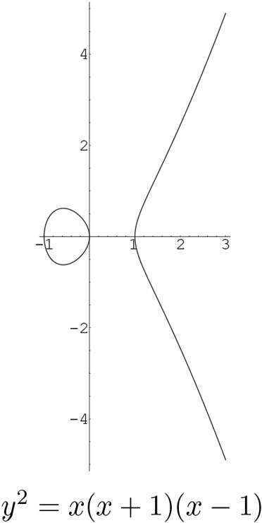

The case of two components (for example, ) occurs when the cubic polynomial has three real roots. The case of one component (for example, ) occurs when the cubic polynomial has only one real root.
For technical reasons that will become clear later, we also include a “point at infinity,” denoted which is most easily regarded as sitting at the top of the . It can be treated rigorously in the context of projective geometry (see [Washington]), but this intuitive notion suffices for what we need. The bottom of the is identified with the top, so also sits at the bottom of the .
Now let’s look at elliptic curves mod where is a prime. For example, let be given by
We can list the points on by letting run through the values and solving for
Note that we again include a point
Elliptic curves mod are finite sets of points. It is these elliptic curves that are useful in cryptography.
Technical point: We assume that the cubic polynomial has no multiple roots. This means we exclude, for example, the graph of Such curves will be discussed in Subsection 21.3.1.
Technical point: For most situations, equations of the form suffice for elliptic curves. In fact, in situations where we can divide by 3, a change of variables changes an equation into an equation of the form See Exercise 1. However, sometimes it is necessary to consider elliptic curves given by equations of the form
where are constants. If we are working mod where is prime, or if we are working with real, rational, or complex numbers, then simple changes of variables transform the present equation into the form However, if we are working mod 2 or mod 3, or with a finite field of characteristic 2 or 3 (that is, or ), then we need to use the more general form. Elliptic curves over fields of characteristic 2 will be mentioned briefly in Section 21.4.
Historical point: Elliptic curves are not ellipses. They received their name from their relation to elliptic integrals such as
that arise in the computation of the arc length of ellipses.
The main reason elliptic curves are important is that we can use any two points on the curve to produce a third point on the curve. Given points and on we obtain a third point on as follows (see Figure 21.1): Draw the line through and (if take the tangent line to at ). The line intersects in a third point Reflect through the (i.e., change to ) to get Define a law of addition on by
Figure 21.1 Adding Points on an Elliptic Curve
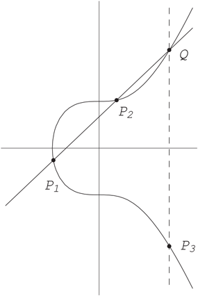
Note that this is not the same as adding points in the plane.
Example
Suppose is defined by Let and The line through and is
Substituting into the equation for yields
which yields Since intersects in and we already know two roots, namely and Moreover, the sum of the three roots is minus the coefficient of (Exercise 1) and therefore equals 1. If is the third root, then
so the third point of intersection has Since we have and Reflect across the to obtain
Now suppose we want to add to itself. The slope of the tangent line to at is obtained by implicitly differentiating the equation for
where we have substituted from In this case, the line is Substituting into the equation for yields
hence The sum of the three roots is 64 (= minus the coefficient of ). Because the line is tangent to it follows that is a double root. Therefore,
so the third root is The corresponding value of (use the equation of ) is Changing to yields
What happens if we try to compute ? We make the convention that the lines through are vertical. Therefore, the line through and intersects in and also in When we reflect across the , we get back Therefore,
We can also subtract points. First, observe that the line through and is vertical, so the third point of intersection with is The reflection across the is still (that’s what we meant when we said sits at the top and at the bottom of the ). Therefore,
Since plays the role of an additive identity (in the same way that 0 is the identity for addition with integers), we define
To subtract points simply add and
Another way to express the addition law is to say that
(See Exercise 17.)
For computations, we can ignore the geometrical interpretation and work only with formulas, which are as follows:
Addition Law
Let be given by and let
Then
where
and
If the slope is infinite, then There is one additional law: for all points
It can be shown that the addition law is associative:
It is also commutative:
When adding several points, it therefore doesn’t matter in what order the points are added nor how they are grouped together. In technical terms, we have found that the points of form an abelian group. The point is the identity element of this group.
If is a positive integer and is a point on an elliptic curve, we can define
We can extend this to negative For example, where is the reflection of across the . The associative law means that we can group the summands in any way we choose when computing a multiple of a point. For example, suppose we want to compute We do the additive version of successive squaring that was used in modular exponentiation:
The associative law means, for example, that can be computed as It also could have been computed in what might seem to be a more natural way as but this is slower because it requires three additions instead of two.
For more examples, see Examples 41–44 in the Computer Appendices.