8 Digital image management and manipulation

This chapter deals with the aspects of digital imaging concerning the images themselves: their representation, manipulation and storage, as they move through the imaging chain. Digital images are, at their most fundamental, sets of numbers rather than physical entities. A key difference between working with traditional silver halide photography and digital images is the vast range of options available, before, during and after image capture. It requires an understanding of all aspects of the imaging chain and the implications of the various processes to ensure optimum results.

Digital image manipulation involves the use of numerical operations to change the appearance or method of representation of an image. It is not, however, confined to the use of image-editing applications such as Photoshop. The image is manipulated at every stage as it progresses through the imaging chain, which can lead to unexpected results and unwanted artefacts. Furthermore, the use of different digital colour spaces throughout makes colour management a complex process. The path through the imaging chain requires choices to be made about image resolution, colour space and file format, as but a few examples. Each decision made about the image will have an impact on any subsequent stages in the workflow, options available and on the quality of the final product. To help to understand the implications of these decisions, this chapter covers six main areas: the nature of the digital image, the digital image file, image workflow, file formats and compression, colour management, and image processing.

The digital image

At its most fundamental, a digital image is simply a set of numerical data, which, when correctly transmitted, interpreted and reproduced by various devices in the digital imaging chain, produce a representation of an original scene or image. The digital images we encounter in photography are known as bitmaps or pixmaps. They are represented as a discrete array of equally spaced pixels, each of which has a set of numbers determining its colour and intensity (Figure 8.1).

Because the numerical data must be stored for every pixel position, image files tend to be quite large if compared to other types of data. The pixel values that we come across if we examine the image information in a typical image-editing application are integers (whole numbers), which will vary in terms of value and range depending upon the colour space employed and the bit depth of the image.

Any type of data within a computer, text or pixel values, is represented in binary digits of information. Binary is a numbering system, like the decimal system. Where decimal numbers can take 10 discrete values from 0 to 9 and all other numbers are combinations of these, binary can

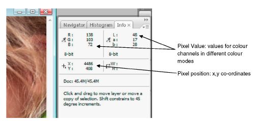
Figure 8.1 A digital image consists of pixels, each of which is represented by a set of numbers determining its colour and intensity.

only take two values, 0 or 1, and all other numbers are combinations of these. The raw image data, i.e. each pixel value, are converted to a string of binary digits when stored or transmitted.

An individual binary digit is known as a bit. The file size of a digital image is equal to the total number of bits required to store the image. The way in which image data are stored is defined by the file format. The process of turning the pixel values into binary code is known as encoding and is performed when an image file is saved.

This basic character of a digital image has a number of implications in terms of its nature and properties when compared with a traditional silver halide photographic image:

Sampling

Digital images are a discrete representation. A key difference between digital and analogue imaging is the fact that the digital image is captured across a regular grid of pixels, in a process known as sampling. In a digital camera, for example, each sensor (corresponding to a pixel) on the array produces a single response proportional to the average amount of light falling on its area, i.e. it takes a sample of the light intensity at that position. Where film ‘grains’ are distributed randomly through a film emulsion and overlap each other to create the impression of continuous tones, the pixels produced are non-overlapping and each is a solid block of colour. As long as the spatial resolution of the image is high enough, the human visual system cannot distinguish between individual pixels and ‘integrates’ them to produce an overall impression of continuous tone. But at lower pixel resolutions, the eye is very efficient at identifying the edges of pixels and images begin to appear pixelated or ‘blocky’. This is particularly noticeable on diagonals, where ‘staircasing’ aliasing artefacts appear. The resolution necessary to prevent these effects depends upon the way in which the image is being viewed – for example, printed images require much higher resolutions than those on screen (see Chapters 2, 6 and 7 for more information on resolution).

Quantization

In a black and white photographic image, a potentially infnite number of tones (or greys) may be produced. Because the silver image grains are very small and layered, they overlap to produce the impression of many different shades of grey.

However, in a digital image, the number of different tones or colours is limited, because each is represented by a fnite-length binary code. As well as being discrete units across the spatial dimensions of the image, pixels can only take certain discrete values. The process of allocating a continuous input range (of intensities) to a discrete output range (of pixel values), which changes in steps, is known as quantization.

The stepped changes in colour values and the non-overlapping nature of the pixels are limiting factors in the quality and resolution of a digital image. The spatial sampling rate is determined by the physical dimensions of the array and individual sensor. The quantization levels depend upon the analogue-to-digital conversion, image processing in the capture device, and ultimately on the bit depth and output file format. Figure 8.2 illustrates the processes of sampling and quantization.

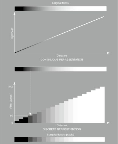
Figure 8.2 Sampling and quantization in a digital image. The image is spatially sampled into a grid of discrete pixels. The continuous greyscale range from the original scene is quantized into a limited set of discrete levels, based on the bit depth of the image.

Bit depth

The bit depth of a digital image refers to the number of binary digits used to represent each pixel, i.e. the length of binary code. The bit depth of an image has important consequences in terms of the number of individual values that may be represented, the colour space and the resulting quality of the image.

Consider a theoretical image represented by only two binary digits per pixel, i.e. a ‘2-bit’ image. Each binary digit may take only two possible values, either 1 or 0. As each pixel value in the image must be represented by a unique code (i.e. the code must relate to one pixel value; no two pixel values should produce the same code, to prevent incorrect decoding when the file is opened), the number of possible values that may be represented depends on the number of different possible two-binary-digit combinations. The possible unique combinations are:

Therefore, the image can only have four different pixel values or tones in it. The relationship between the number of bits allocated to each pixel and the number of unique codes that are produced by that number of bits is defined by:

where k = number of bits and L = number of levels. Therefore, 2 bits produce 2² = 4 and 7 bits produce 2⁷ = 128. Some examples of tonal ranges produced by different bit depths are illustrat in Figure 8.3.

Eight bits is usually regarded as the minimum number necessary to adequately reproduce a continuous tone image. Our ability to discriminate between individual tones and colours is complicated because it is affected by many factors, including the ambient lighting level; under normal daylight conditions the human visual system needs the tonal range from shadow to highlight to be divided into between 120 and 190 different levels to see continuous tone. Fewer than this and contouring artefacts (sometimes termed posterization) become apparent, appearing as visible jumps between tone or colour levels in smoothly graduated areas. These are particularly noticeable to the human visual system, which has in-built edge detection mechanisms to enhance the effect. Note that our discrimination of tone is much more sensitive than that of colour, hence it is sometimes possible to achieve some level of compression by separating out colour from tonal information and reducing the number of colours represented.

Figure 8.3 The bit depth of the image defines the number of unique binary codes and the number of discrete grey levels or pixel values that may be represented.

An example of a 2-bit image is illustrated in Figure 8.4(a). It is quite obvious that four different levels are not enough to produce the impression of continuous tone. Figure 8.4(b) and (c) show the same image with 4 and 8 bits per pixel. The 256 levels produced by 8 bits are adequate to produce the representation of continuous tone that we would expect from a photographic image.

File size

The file size of the raw image data in terms of bits can be worked out using the following formula:

File size = (No. of pixels) × (No. of colour channels) × (No. of bits / colour channel).

Eight bits make up 1 byte, 1024 bytes equal 1 KB, 1024 KB equal 1 MB and so on. Therefore, file size can then be converted into megabytes by dividing by (8 × 1024 × 1024).

Image data file size is therefore dependent on two factors: pixel resolution and bit depth of the image. It can be inspected by selecting image size in an application such as Photoshop. However, it should be noted that the size of the image data may be significantly different to the size of the image file (the size of the storage space on disk). Once saved to a particular format,

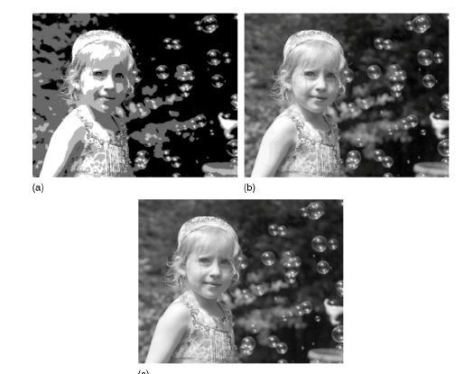
Figure 8.4 A greyscale image represented with only 2 bits per pixel (a), 4 bits per pixel (b) and 8 bits per pixel (c). ‘Anja’ © Elizabeth Allen.

it will contain other information, which may add to the file size, such as headers, tags, EXIF data, etc. Furthermore, very few file formats save the raw data without any processing at all. The data are usually compressed, by rearranging to store more efficiently, hence saving space and reducing file size. The file format will determine both the compression method and the additional data to be saved.

Eight-bit versus 16-bit workflow

For an RGB image, 8 bits per channel gives a total of 24 bits per pixel and produces over 16 million different colours. Where photographic quality is the intention, typical digital images are either 8 or 16 bits per channel.

Usually, image sensors will capture more than 8 bits. It is the process of quantization by the analogue-to-digital converter that allocates the tonal range to 8 or 16 bits. The move towards 16-bit imaging is possible as a result of better storage and processing in computers – working with 16 bits per channel doubles the file size. Eight bits is adequate to represent smoothly changing tone, but as the image is processed through the imaging chain, particularly tone and colour correction, pixel values are reallocated, which may result in some pixel values missing completely, causing posterization. Starting with 16 bits produces a more finely sampled tonal range, helping to avoid this problem. Figure 8.5 illustrates the difference between an 8-bit and a 16-bit image after some image processing. Their histograms show this particularly well: the 8-bit histogram clearly appears jagged, as if beginning to break down, while the 16-bit histogram remains smooth.

Using a 16-bit workflow can present an opportunity to improve and maintain image quality, but may not be available throughout the imaging chain. Certain operations, particularly filtering, are not available for anything but 8-bit images. Additionally, 16-bit images are not supported

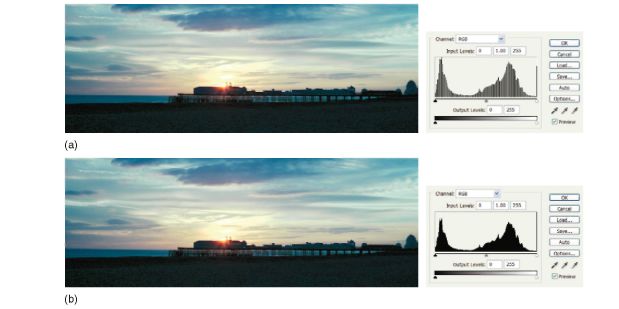
Figure 8.5 (a) Processing operations such as levels adjustments can result in the image histogram of an 8-bit image having a jagged appearance and missing tonal levels (posterization). (b) Sixteen-bit images have more tones available, therefore the resulting histogram is smoother and more complete, indicating fewer image artefacts. Image © Elizabeth Allen

by all file formats. At the time of writing, 16-bit output is only available with a limited range of printers, display devices and specific operating systems. However, this situation is likely to change. Archiving 16-bit images in a wide-gamut colour space can help to ensure that they may exploit the improved capabilities of operating systems and output devices in the future.

Image modes

Digital image data consist of sets of numbers representing pixel values. The image mode provides a global description of what the pixel values represent and the range of values that they can take. The mode is based on a colour model and defines colours numerically. The common image modes are as follows:

• RGB – three colour channels representing red, green and blue values. Each channel contains 8 or 16 bits per pixel.
• CMYK – four-channel mode. Values represent cyan, magenta, yellow and black, again 8 or 16 bits per pixel per channel.
• LAB – three channels, L representing tonal (luminance) information, and a and b colour (chrominance) information.
• HSL (andvariations) – these three-channel models produce colours by separating hue from saturation and lightness. These are the types of attributes we often use to describe colours verbally and so can be more intuitive to understand and visualize colours represented in red, green and blue. However, they are very non-standardized and do not relate to the way any digital devices produce colour, so tend not to be widely used in photography.
• Greyscale – this is a single-channel mode, where pixel values represent neutral tones, again with a bit depth of 8 or 16 bits per pixel.
• Indexed – these are also called paletted images, and contain a much reduced range of colours to save on storage space and are therefore only used for images on the web, or saturated graphics containing few colours. The palette is simply a look-up table (LUT) with a limited number of entries (usually 256); at each position in the table three values are saved, representing RGB values. At each pixel, rather than saving three values, a single value is stored, which provides an index into the table, and outputs the three RGB values at that index position to produce the particular colour. Converting from RGB to indexed mode can be performed in image-processing software, or by saving in the Graphics Interchange Format (GIF) file format.

Some of the colour modes correspond to particular colour spaces, for example LAB, which specifes colours in the CIELAB standard colour space based on the CIE (Commission International de L’Eclairage) system of colorimetry. Others, such as RGB and CMYK, are modes that encompass many device-dependent colour spaces, For example, all cameras, scanners and displays are RGB devices, but each individual device has its own RGB colour space. Colour spaces and colour management are discussed later in the chapter.

Layers and alpha channels

Layers are used in image-processing applications to make image adjustments easier to fine-tune, to selectively adjust particular regions of the image and to allow the compositing of elements from different images in digital montage. Layers can be thought of as ‘acetates’ overlying each other, on top of the image, each representing different operations or parts of the image. Layers can be an important part of the editing process, but vastly increase file size, and therefore are not usually saved after the image has been edited to its final state for output – the layers are merged down. If the image is in an unfinished state, then file format must be carefully selected to ensure that layers will be preserved.

Alpha channels are an extra greyscale channel within the image. They are designed for compositing and can perform a similar function to layers, but are stored separately and can be saved and even imported into other applications, so are much more permanent and versatile. They can be used in various different ways – for example, to store a selection which can then be edited later. They can also be used as masks when combining images, the value at each pixel position defning how much of the pixel in the masked image is blended or retained. They are sometimes viewed as transparencies, with the value representing how transparent or opaque a particular pixel is. Like layers, alpha channels increase file size. Again, support depends on the file format selected, although more formats support alpha channels than layers.

Image workflow

The term workflow refers to the progress of the image through the imaging chain, and the steps taken from capture to output. The complex process of digital image production encompasses many different stages, and within each there are a myriad of different options. A well-thought-out and carefully defined workflow provides a methodical approach to image management, and helps to ensure that image quality is maintained.

The capture settings are important as limiting factors in the overall quality of the final image. As described below, there is always a trade-off between maximum quality and speed of processing. It is therefore important to decide on which is a priority at the very beginning, as this will determine, for example, whether to capture RAW files or a compressed file format such as JPEG (Joint Photographic Experts Group).

There are a number of basic image adjustments which are necessary for the optimization of almost all digital images. Such processes correct for problems at capture, the noise and sharpness characteristics of the imaging optics, and in some cases for artefacts introduced by other devices or processes. In many cases, these operations can be performed at several points in the imaging chain. A good workflow will help to determine the optimal point for the operations to be carried out in the context of the particular image output and the devices being used, ensuring that they are not repeated unnecessarily. This can help to allow the automation of some processes. For example, if speed is a priority and many images are to be captured under the same conditions, then it may be feasible to apply image adjustments such as tone curves in the camera settings. Alternatively, in a studio setting, the same set of operations, from processing RAW files to archiving them, might be performed using batch processing in an image-editing application.

Another important aspect of workflow is colour management, which aims to ensure that image colours are correctly specified and communicated between different devices and imaging chains. Digital colour reproduction is a complicated problem, not least because of the huge variety of input and output devices available, each of which has its own device colour space. The colour management system is made up of software and hardware devices designed to measure and translate colour values between all the different devices. The International Colour Consortium (ICC) provides a standardized framework for colour management systems, which is discussed later in the chapter. A workflow which utilizes ICC colour management is nowadays essential for good colour reproduction in most digital imaging tasks (only in research and some scientific applications, where images are transmitted between a small loop of specified devices, is this less relevant).

Your workflow will be partially determined by the devices you use, but just as important is the use of software at each stage. The choices you make will also depend upon a number of other factors, such as the type of output, necessary image quality and image storage requirements.

Software

There is no standardization in terms of software, but the range of software used by most photographers has gradually become more streamlined as a result of industry working practices, and therefore a few well-known software products dominate at the professional level at least. For the amateur, the choice is much wider and often devices will be sold with lite’ versions of the professional applications. However, software is not just important at the image-editing stage, but at every stage in the imaging chain. Some of the software that you might encounter through the imaging chain includes:

• Digital camera software to allow the user to change settings.
• Scanner software, which may be proprietary or an independent software such as Vuescan or Silverfast.
• Organizational software, to import, view, name and file images in a coherent manner. In applications such as Adobe Bridge, images and documents can also be managed between different software applications, such as illustration or desktop publishing packages. Adobe Lightroom combines the management capabilities of other packages to organize workflow with a number of image adjustments.
• RAW processing software, both proprietary and as plug-ins for image-processing applications.
• Image-editing software. A huge variety of both professional and lite versions exist. Within the imaging industry, the software depends upon the type and purpose of the image being produced. Adobe Photoshop may dominate in the creative industries, but forensic, medical and scientific imaging have their own types of software, such as NIH image (Mac)/Scion Image (Windows) and Image J, which are public-domain applications optimized for their particular workflows.
• System software, which controls how both devices and other software applications are set up. Database software, to organize, name, archive and back up image files.
• Colour management software, for measuring and profling the devices used in the system.

It is clearly not possible to document the pros and cons, or detailed operation, of all software available to the user, especially as new versions are continually being brought out, each more sophisticated than the last. The last three types of software in the list, in particular, are unlikely to be used by any but the most advanced user and require a fair degree of knowledge and time to implement successfully. It is possible, however, to define a few of the standard image processes that are common from application to application and that it is helpful to understand. In terms of image processing, these may be classed as image adjustments and are a generic set of operations that will usually be performed by the user to enhance and optimize the image. The main image adjustments involve resizing, rotating and cropping of the image, correction of distortion, correction of tone and colour, removal of noise and sharpening. These are discussed in detail later in the chapter. The same set of operations is often available at multiple points in the imaging chain, although they may be implemented in different forms.

In the context of workflow and image quality, it is extremely useful to understand the implications of implementing a particular adjustment at a particular point. Some adjustments may introduce artefacts into the image if applied incorrectly or at the wrong point. Fundamentally, the order of processing is important. They may also limit the image in terms of output, something to be avoided in an open-loop system. Another consideration is that certain operations may be better performed in device software, because the processes have been optimized for a particular device, whereas others may be better left to a dedicated image-processing package, because the range of options and degree of control is much greater. Ultimately, it will be down to users to decide how and when to do things, depending on their system, a bit of trial and error, and ultimately their preferred methods of working.

General considerations in determining workflow

Because of the huge range of different digital imaging applications, it is impossible to define one optimal workflow. Some workflows work better for some types of imaging and most people will establish their own preferred methods of working. Ultimately your workflow should make the process of dealing with digital images faster and more efficient, and it should work towards optimum image quality for the required output – if it is known. Figure 8.6 illustrates a general digital imaging workflow from capture to output. As shown, at each stage there are many options: some stages are workflows in themselves.

Capture for output workflows

When digital imaging first began to be adopted by the photographic industry, the imaging chain was restricted in terms of hardware available. At a professional level the chain would consist of a few high-end devices, usually with a single input and output. These were called closed-loop imaging systems and made the workflow relatively simple. The phrase ‘closed loop’ was originally coined to refer to methods of colour management, but can also be applied to the overall imaging chain, of which colour management is one aspect. Usually, a closed-loop system is run by a single operator who, having gained knowledge of how the devices work together over time, can control the imaging workflow, in a similar way to the quality control processes implemented in a photographic film processing lab, to get required results and correct for any drift in colour or tone from any of the devices.

In a closed-loop system, where the output image type and the output device are known, it is possible to use a capture for output approach to workflow, which means that all decisions made at the earlier stages in the imaging chain are optimized to the requirements of that output. Today we don’t tend to work with closed-loop systems, but the same sort of approach can be applied to workflow, if the output is known and speed is a priority.

For example, when shooting for web output, it is possible to save time and space by capturing at quite a low resolution and saving the image as a JPEG file. Similarly, if it is known that a scanned image is to be printed to a required size on a particular printer, the image can be captured with exactly the number of pixels required for that output, converted into the printer colour space immediately and, by doing so, help to optimize image quality and reduce the number of out-of-gamut colours generated. In both cases the image should need less postprocessing work if any, and will be ready to be used straight away, correct for the required output. This approach is simple, fast and efficient. However, as soon as other devices start to be added to the imaging chain, or the image is required for a different type of output, a capture for output workflow starts to fail in terms of effciency and the resulting images may no longer be of a suitable quality.

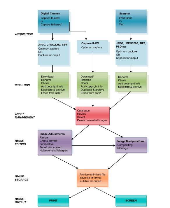
Figure 8.6 Digital imaging workflow. This diagram illustrates some of the different stages that may be included in a workflow. The options available will depend on software, hardware and imaging application.

Optimum capture workflows

If the output is unknown, then it becomes important to maintain fexibility in the imaging chain for multiple different outputs. Alternatively, a high quality output may be required. To maintain both fexibility and maximum quality an optimum capture workflow is more appropriate.

The use of multiple input and output devices is commonplace by both amateurs and professionals, and these types of imaging chains are known as open-loop systems. Often, an image may take a number of different forms. For example, it may be that a single image will need to be output as a low-quality version with a small file size to be sent as an attachment to an email, a high-quality version for print and a separate version to be archived in a database. Open-loop systems are characterized by the ability to adapt to change. In such systems, it is no longer possible to optimize input for output, and in this case the approach has to be to optimize quality at capture and then to ensure that the choices made further down the chain do not restrict possible output or compromise image quality. Often, multiple copies of an image will exist, for the different types of output, but also multiple working copies, at different stages in the editing process. This ‘non-linear’ approach has become an important part of the image-processing stage in the imaging chain, allowing the photographer to go back easily and correct mistakes or try out many different ideas. Many photographers therefore find it is simply easier to work at the highest possible quality available from the input device, and then make decisions about reducing quality or file size where appropriate later on. At least by doing this, they know that they have the high-quality version archived should they need it. This requires a decent amount of storage space, time and skill, in both capture and subsequent processing.

Rendered versus unrendered image capture: capturing RAW

At the time of writing, some compact and bridge cameras, and almost all DSLRs and larger format cameras, provide the option to capture RAW files as well as JPEGs. In a few cases other formats such as JPEG 2000 and TIFF are also available. The choice between RAW and JPEG is a good example of a trade-off between quality and speed.

On a general level, it is a decision about whether to save fully colour rendered, processed and (in most cases) lossy compressed images, ready for output, or unrendered images, which require more processing before they are viewable and ready for output.

As described in previous chapters, nearly all digital cameras have a colour filter array in front of the image sensor, and at each pixel site only one colour is captured. The captured values are sampled and quantized in an analogue-to-digital converter and these are the ‘raw’ image data in a relatively unprocessed state, as close as possible to the sensor response to the scene. To produce the three colour values required for the rendered RGB image, a process of interpolation is employed to calculate the missing values at each pixel site (known as demosaicing and described in Chapters 2 and 6). This process is illustrated in Figure 8.7.

Prior to, or in some cases in conjunction with, demosaicing, a significant amount of image processing is applied. To produce a rendered image in file formats other than RAW, this is applied in the camera, in the firmware and digital signal processor. The photographer has limited control through the camera settings. Examples include exposure, colour space, white balance, noise removal and sharpening, which are applied to the image before it is saved.

If speed is of the essence and some loss of image quality is acceptable, then capturing to JPEG may be the best option. The image files are small, fully processed and can go straight to an

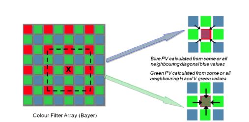
Figure 8.7 The demosaicing process to calculate missing colour channel values at each pixel site in an image captured using a Bayer array. This process occurs in-camera for rendered file formats such as JPEG. With RAW files, demosaicing is performed during postprocessing in RAW conversion software.

output device. However, if there are any mistakes during acquisition, the degree to which they may be corrected is limited. Too much adjustment can be detrimental to the image quality, which is already compromised by the lossy JPEG compression process.

RAW files bypass some of the in-camera processing, producing data from the camera that are much closer to what was actually ‘seen’ by the image sensor. The RAW file consists of the raw pixel data and a header, which contains information about the camera and capture conditions. RAW files store only the single value per pixel through the colour filter array; much of the processing described above and the demosaicing are performed afterwards in RAW conversion software (see Figures 8.8 and 8.9), which may be a stand-alone application from the camera manufacturer, or a plug-in in an editing application. Because colour interpolation has not been performed, the data in a RAW file are a third of the size of that in a rendered RGB file format and despite the additional capture information included with the data the resulting file size will be significantly smaller than the equivalent TIFF.

There are a number of advantages to working with RAW files. The most obvious is that it allows the photographer control over the processing applied to the image at capture. Decisions over aspects such as colour space, white point and sharpening methods may be deferred until after the image capture stage. Each may be fine-tuned interactively, previewing the results on a large calibrated screen prior to finalizing the image (see Figure 8.9).

RAW conversion software also allows alteration of exposure, tone, contrast and colour. The image is optimized by the user, meaning that the numbers of decisions made at capture are reduced and mistakes can be corrected to some extent afterwards. Furthermore, because some of the image adjustments are applied during RAW conversion rather than in a separate image-editing application such as Photoshop, they happen in conjunction with demosaicing and this can help to maximize image quality.

A further advantage lies in the fact that until the image is demosaiced, more of the full dynamic range of the sensor is available, which may be between 10 and 14 bits, or more. This means that it is possible to alter exposure during RAW conversion. If the original exposure clipped either end of the tonal range, the entire range can be shifted up or down, slightly over-or underexposing to correct the clipping. When a high-dynamic-range scene is captured to

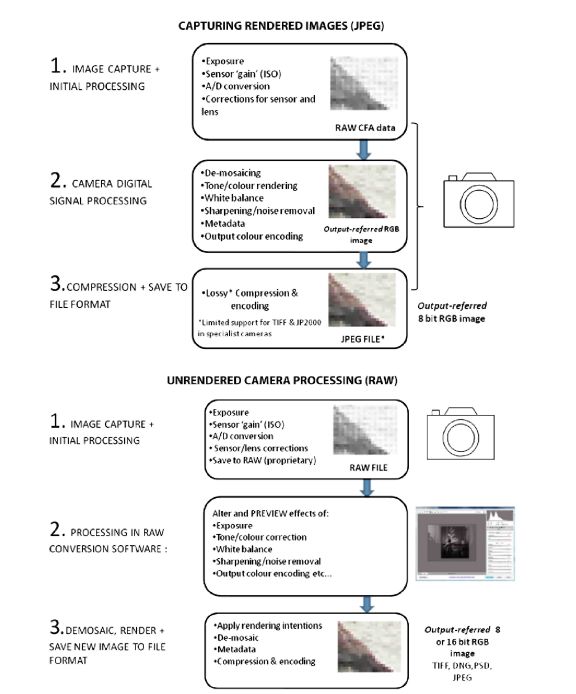
Figure 8.8 A comparison of processing workflow for RAW and JPEG captured files.

a format such as JPEG, clipped highlights or shadows cannot be retrieved when the overall brightness or contrast of the image is changed. This is illustrated in Figure 8.10.

Perhaps one of the most important aspects of working with RAW files is that nothing is finalized until the image is saved to a rendered format such as TIFF or PSD. This means that image editing is non-destructive. In fact, all that happens in the RAW converter until the file is saved is a preview of whatever processing is to be applied. A new image file is created when the file is saved, but the RAW data remain unchanged and available for reprocessing at any time. Several different versions of the image with different processing may be saved, without affecting the original image data. It is clear that this offers photographers versatility and control over the image capture stage. The downside of capturing in RAW is that it requires skill and knowledge to carry out the processing. Additionally, as it is not yet a standardized

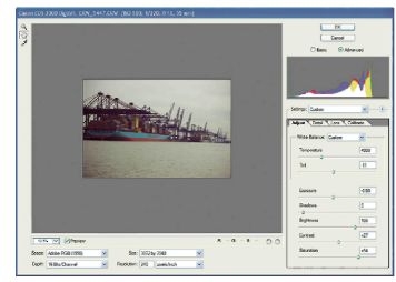
Figure 8.9 Camera RAW plug-in interface.

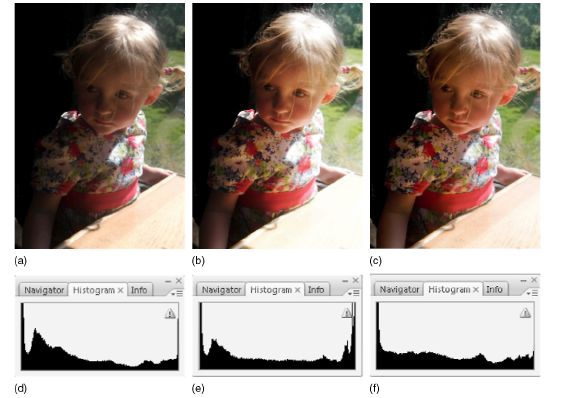
Figure 8.10 The results of tonal adjustments to an underexposed image applied to an 8-bit JPEG file and a RAW captured file. (a) Original image. (b) Results of contrast and brightness adjusted from JPEG capture. (c) The exposure is corrected and contrast adjusted using levels and curved during RAW conversion. (d) Original histogram. (e) JPEG adjusted histogram. (f) RAW adjusted histogram. Image © Elizabeth Allen

format, each camera manufacturer has a proprietary RAW file optimized for their particular camera, with a different type of software to perform the image processing, which complicates things if you use more than one camera. Adobe has developed Camera RAW software, which provides a common interface for the majority of modern RAW formats (but not yet all). It makes the process simpler, but you may achieve better results using the manufacturer’s dedicated software. Because of the proprietary nature of the format it is also wise to exercise caution when using RAW to archive images. Resaving the files as Adobe Digital Negative (DNG) files, which are a form of universal RAW file, may be advisable in case the proprietary format you are using becomes obsolete.

Standards

Alongside the development of open-loop methods of working, imaging standards have become more important. Bodies such as the International Organization for Standardization (ISO), the International Colour Consortium (ICC) and the JPEG work towards defning standard practice and imaging standards in terms of technique, file format, compression and colour management systems. Their work aims to simplify workflow and ensure interoperability between users and systems, and it is such standards that define, for example, the file formats commonly available in the settings of a digital camera, or the standard working colour spaces most commonly used in an application such as Adobe Photoshop.

Standards are therefore an important issue in designing a workflow. They allow a photographer to match their processes to common practice within the industry and help to ensure that their images will ‘work’ on other people’s systems. For example, by using a standard file format, you can be certain that the person to whom you are sending your image will be able to open it and view it in most imaging applications. By attaching a profile to your image, you can help to make sure that the colour reproduction will be correct when viewed on someone else’s display (assuming that they are also working on ICC standards and have profiled their system of course).

Image capture

Scanning workflow has been covered in Chapter 7, therefore this section concentrates on workflow using a digital camera. When shooting digitally, there are many more decisions to be made and steps to be taken than when using a film camera. Not all the steps described below will be relevant to a particular workflow, depending on how the images are to be captured. Quite fundamental to this is whether the images are being shot to a memory card or directly to a computer. Also, as mentioned earlier, the decision to shoot RAW or JPEG files has significant implications in terms of capture workflow.

Tethered shooting

In a studio setting and particularly with larger format cameras, it is often possible to work with the camera tethered directly to a computer, shooting images using remote capture software. The images are captured and downloaded directly to the computer, bypassing the need for a memory card and therefore cutting out the entire process of capturing, storing and downloading images. Image capture is performed using some form of remote capture software, which is usually supplied by the camera manufacturer and images may then be imported directly into an image management software – for example, Adobe Lightroom. Note that Lightroom version 3 includes the remote capture function, allowing the two steps to be performed together. An important preparation stage, aside from the necessary practical steps, is to configure the software. This includes setting preferences and setting up the file management system, creating folders for the images to be captured into, and defning the naming protocols for each image file. There are many approaches to this, depending on the applications being used, and each photographer will develop their own system. It is a vital step in ensuring that the images are correctly stored and easy to find and retrieve. It is also possible with some DSLRs in conjunction with a specialized unit to transmit images wirelessly, although transmission rates can be rather slow.

Formatting the card

Assuming that tethered shooting is not an option, capture will be to a memory card. There are a variety of different types of memory card available, depending upon the camera system being used. These can be bought reasonably cheaply and it is useful to keep a few spare, especially if using several different cameras. It is important to ensure that any images have been downloaded from the card before beginning a shoot, and then perform a full erase or format on the card in the camera. It is always advisable to perform the erase using the camera itself. Erasing from the computer when the camera is attached to it may result in data such as directory structures being left on the card, taking up space, and useless if the card is used in another camera.

Setting image resolution

Image resolution is determined by the number of pixels at image capture, which is obviously limited by the number of pixels on the sensor. In some cameras, however, it is possible to choose a variety of different resolutions at capture, which has implications for file size and image quality. Unless capturing for a particular output size and short of time or storage space, it is better to capture at the native resolution of the sensor (which can be found from the camera’s technical specifications), as this will ensure optimum quality and minimize interpolation.

Setting capture colour space

The colour space setting defines the colour space into which the image will be captured and is important when working with a profiled (colour managed) workflow. Usually, there are at least two possible standard RGB spaces available: sRGB and Adobe RGB (1998). sRGB was originally developed for images to be displayed on screen and therefore has a relatively small gamut characteristic of a cathode ray tube (CRT) type display. There is usually fairly significant mismatch between printer gamuts and display gamuts, and images captured in sRGB, when printed, can sometimes appear dull and desaturated. Adobe RGB (1998) is a larger colour space, with a gamut increased to better cover the range of colours reproduced by printers as well. Unless you know that the images you are capturing are only for displayed output, Adobe RGB (1998) is usually the optimum choice.

Some DSLRs and larger formats have their own RGB colour profile available as a colour space setting and better results may be obtained by using this. Once the image is imported into an application such as Photoshop it can be converted to a working standard RGB colour space. Alternatively, if the sensor colour space is being used, the image may be kept in this colour space throughout the imaging chain, changing only when the image is output to print.

It is important to note that, when capturing RAW files, setting the colour space will not influence the results. When the RAW file is opened up in RAW conversion software, the profile of the colour space selected in the camera will be used to create the preview image. However, the underlying data will remain unchanged. The colour space can be changed at this point and will only affect the image when the file is finalized and saved.

Setting white balance

As discussed in Chapter 1, the spectral quality of white light sources varies widely. Typical light sources range from colour temperatures of around 2000 or 3000 K (typical of tungsten), which tend to be yellowish in colour up to 6000 or 7000 K for bluish light sources, such as daylight or electronic flash. Our eyes adjust to these differences (in a process known as chromatic adaptation), so that we always see the light sources as white unless they are viewed together. However, image sensors do not adapt automatically. Colour film is balanced for a particular light source. The colour response of digital image sensors is altered for different sources using the white balance setting. This is usually performed on the image data in the digital signal processing unit; alternatively, it can sometimes be achieved by applying different amounts of gain to the analogue signals prior to A/D conversion. By effectively boosting the signals from the red-, green- and blue-sensitive pixels by different amounts, the relative amounts that each contributes to a pixel changes, and the overall colour balance of the image is altered.

White balance may be set in a number of different ways.

White balance presets

These are preset colour temperatures for a variety of typical photographic light sources and lighting conditions. Using these presets is fine if they exactly match the lighting conditions. It is important to note that colour temperature may vary for a particular light source. Daylight may have a colour temperature from approximately 3000 up to 12 000 K, depending upon the time of day, year and distance from the equator. Tungsten lamps also vary, especially as they age.

Auto white balance

The camera takes a measurement of the colour temperature of the scene and sets the white balance automatically. This can work very well, is reset at each shot, and so adapts as lighting conditions fluctuate.

Custom white balance

Most DSLRs have a custom white balance setting. The camera is zoomed in on a white or neutral object in the scene, a reference image is taken and this is then used to set the white balance. This can be one of the most accurate methods for setting the white balance.

White balance through RAW processing

When shooting RAW, it is not necessary to set white balance as this is one of the processes performed in the RAW editor post-capture using sliders; therefore, leaving the camera on auto white balance is probably the best option. The average colour temperature of the scene will be displayed in the RAW editor, but can be fine-tuned prior to the image being finalized. Custom white balancing may also be performed during RAW conversion. This is best achieved using a neutral (mid-grey) rather than a white area, as highlight areas may have colour casts that are difficult to detect but profoundly affect the overall colour balance of the image.

Setting ISO speed

As for film, the ISO setting ensures correct exposure across a variety of different lighting levels. However, it is not possible to change the sensitivity of the sensor. It will have a native sensitivity; usually the lowest ISO setting and other ISO speeds are achieved by amplifying the signal response. Unfortunately this also amplifies the noise levels within the camera. Some of the noise is present in the signal itself and is more noticeable at low light levels. Digital sensors are also susceptible to other forms of noise caused by the electronic processing within the camera. Some of this is processed out on the chip, but noise can be minimized by using low ISO settings. Above an ISO of 400, noise is often problematic. It can be reduced with noise filters during postprocessing, but this causes some blurring of the image.

ISO speed settings equate approximately to film, but are not exact as sensor responses vary. For this reason, the camera exposure meter is better than an external light meter for establishing correct exposure.

Setting file format

The file format is the way in which the image will be ‘packaged’ and has implications in terms of file size and image quality. The format is set in the image parameters menu before capture and will define the number of images that can be stored on the memory card. The main formats available at image capture are commonly JPEG, TIFF (Tagged Image File Format) (some cameras), RAW and RAW + JPEG (some cameras).

Exposure: using the histogram

One of the great advantages of working digitally is the opportunity to immediately review an image, check the exposure and reshoot if necessary. However, image review (unless shooting tethered to a computer) usually happens on a small LCD screen on the back of the camera and this is an inaccurate way of judging either contrast or potential clipping of highlights or shadows. Much better results may be achieved using the histogram to assess exposure. In many cameras, most DSLRs and in remote capture software, it is possible to display histograms alongside the image, often with an option for an out-of-gamut warning, which highlights pixels in the image that are clipped or out of gamut. A correctly exposed image will have all the contained pixels within the limits of the histogram and will stretch across most of the extent of the histogram, as shown in Figure 8.11(a). An underexposed image will have its levels concentrated at the left-hand side of the histogram, indicating many dark pixels, and an

Figure 8.11 (a) Image histogram showing correct exposure, producing good contrast and a full tonal range. (b) Histogram indicating underexposure. (c) Histogram indicating overexposure.

overexposed image will be concentrated at the other end. If heavily under- or overexposed, the histogram will have a peak at its far end, indicating that either shadow or highlight details have been clipped (Figure 8.11(b, c)). The narrowness of the spread of values across the histogram indicates a lack of contrast. If the histogram is narrow or concentrated at either end, then it indicates that the image should be reshot to obtain a better exposure and histogram. It is particularly important not to clip highlights within a digital image.

Image compression

There are many different formats available for the storage of images. As discussed previously, the development of file format standards allows use across multiple platforms to allow interoperability between systems. Many standards are free for software developers and manufacturers to use, or may be used under licence. Importantly, the code on which they are based is standardized, meaning that a JPEG file from one camera is similar or identical in structure to a JPEG file from another and will be decoded in the same way.

There are other considerations when selecting file format. The format may determine, for example, maximum bit depth of the image, colour space support, whether lossless or lossy compression has been applied, whether layers are retained separately or flattened, whether alpha channels are supported and a multitude of other information that may be important for the next stage. These factors will affect the final image quality: whether the image is identical to the original or additional image artefacts have been introduced, whether it is in an intermediate editing state or in its final form and, of course, the image file size. Whichever format is selected, it will contain more than just the image data and therefore file sizes vary significantly from the file size calculated from the raw data, depending on the way that the data is ‘packaged’, whether the file is compressed or not and also the content of the original scene (Figure 8.12).

The large size of image files has led to the development of a range of methods for compressing images, and this has important implications in terms of workflow. There are two main classes of compression. The first is lossless compression, an example being the LZW

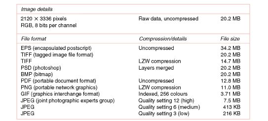
Figure 8.12 File sizes using different formats. The table shows file sizes for the same image saved as different file formats.

compression option incorporated in TIFF, which organizes image data more efficiently without removing any information, therefore allowing perfect reconstruction of the image. Lossy compression, such as that used in the JPEG compression algorithm, discards information that is less important visually, achieving much greater compression rates with some compromise to the quality of the reconstructed image. There is a trade-off between resulting file size and image quality in selecting a compression method. The method used is usually determined by the image file format. Selecting a compression method and file format therefore depends upon the purpose of the image at that stage in the imaging chain.

Lossless compression

Lossless compression is used wherever it is important that the image quality is maintained at a maximum. The degree of compression will be limited, as lossless methods tend not to achieve compression ratios of much above 2:1 (that is, the compressed file size is half that of the original) and the amount of compression will also depend upon image content. Generally, the more fine

Figure 8.13 Compressed file size and image content. The contents of the image will affect the amount of compression that can be achieved with both lossless and lossy compression methods.

detail that there is in an image, the lower the amount of lossless compression that will be possible (Figure 8.13). Images containing different scene content will compress to different file sizes.

If it is known that the image is to be output to print, then it is usually best saved as a lossless file. The only exception to this is some images for newspapers, where image quality is sacrificed for speed and convenience of output. As a rule, if an image is being edited, then it should be saved in a lossless format (as it is in an intermediate stage). Some lossless compression methods can actually expand file size, depending upon the image; therefore, if image integrity is paramount and other factors such as the necessity to include active layers with the file are to be considered, it is often easier to use a lossless file format with no compression applied. Because of this, the formats commonly used at the editing stage will either incorporate a lossless option or no compression at all. File formats that do include lossless compression as an option include: TIFF, PNG (Portable Network Graphics) and a lossless version of JPEG 2000.

If an image is to be archived, then it is vital that image quality is maintained and TIFF or RAW files will usually be used. In this case, compression is not usually a key consideration. Image archiving is dealt with in Chapter 13.

Lossy compression

There are certain situations, however, where it is possible to get away with some loss of quality to achieve greater compression, which is why the JPEG format is almost always available as an option in digital cameras. Lossy compression methods work on the principle that some of the information in an image is less visually important, or even beyond the limits of the human visual system, and use clever techniques to remove this information, still allowing reasonable reconstruction of the images. These methods are sometimes known as perceptually lossless, which means that, up to a certain point, the reconstructed image will be virtually indistinguishable from the original, because the differences are so subtle (Figure 8.14).

Figure 8.14 Perceptually lossless compression: (a) Original image. (b) This image compressed using JPEG to a compression ratio of 23:1 (i.e. the file size is 1/23 the size of the uncompressed size). Most observers would not be able to see any difference between the two.

The most commonly used lossy image compression method, JPEG, allows the user to select a quality setting based on the visual quality of the image. Compression ratios of up to 100:1 are possible, with a loss in image quality that increases with decreasing file size (Figure 8.15).

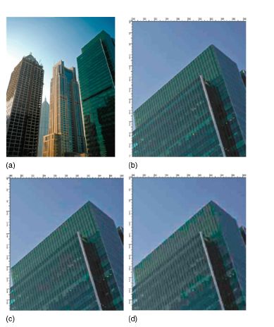
Figure 8.15 Loss in image quality compared to file size. When compressed using a lossy method such as JPEG, the image begins to show distortions that are visible when the image is examined close up. The loss in quality increases as file size decreases. (a) Original image, 3.9 MB. (b) JPEG Q6, 187 KB. (c) JPEG Q3, 119 KB. (d) JPEG Q0, 63.3 KB.

More recently, JPEG 2000 has been developed, the lossy version of which allows higher compression ratios than those achieved by JPEG, again with the introduction of errors into the image and a loss in image quality. JPEG 2000 seems to present a slight improvement in image quality, but more importantly is more fexible and versatile than JPEG. JPEG 2000 has yet to be widely adopted, but is likely to become more popular over the next few years as the demands of modern digital imaging evolve.

Compression artefacts and workflow considerations

Lossy compression introduces error into the image. Each lossy method has its own characteristic artefacts. How bothersome these artefacts are is very dependent on the scene itself, as certain types of scene content will mask or accentuate particular artefacts. The only way to avoid compression artefacts is not to compress so heavily.

JPEG divides the image up into 64 × 64 pixel blocks before compressing each one separately. On decompression, in heavily compressed images, this can lead to a blocking artefact, which is the result of the edges of the blocks not matching exactly as a result of information being discarded from each block. This artefact is particularly visible in areas of smoothly changing tone. The other artefact common in JPEG images is a ringing artefact, which tends to show up around high-contrast edges as a slight ‘ripple’. This is similar in appearance to the halo artefact that appears as a result of oversharpening and therefore does not always detract from the quality of the image in the same way as the blocking artefact.

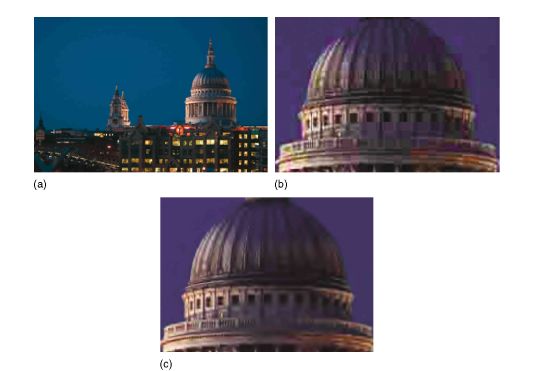
Figure 8.16 (a) Uncompressed image. (b, c) Lossy compression artefacts produced by JPEG (b) and JPEG 2000 (c).

One of the methods by which both JPEG and JPEG 2000 achieve compression is by separating colour from tonal information. Because the human visual system is more tolerant to distortion in colours than tone, the colour channels are then compressed more heavily than the luminance channel. This means, however, that both formats can suffer from colour artefacts, which are often visible in neutral areas in the image.

Because JPEG 2000 does not divide the image into blocks before compression, it does not produce the blocking artefact of JPEG, although it still suffers to some extent from ringing, but the lossy version produces its own ‘smudging’ artefacts (Figure 8.16).

Because of these artefacts, lossy compression methods should be used with caution. In particular, it is important to remember that every time an image is opened, edited and resaved using a lossy format, further errors are incurred. Lossy methods are useful for images where file size is more important than quality, such as for images to be displayed on web pages or sent by email. The lower resolution of displayed images compared to printed images means that there is more tolerance for error.

Choosing file format

In the brief history of digital imaging, many image file formats have been developed. Ultimately the photographic industry has tailored its use to just a few different types. Because of the properties of each, they have distinct functions within the imaging chain.

Figure 8.17 File formats for an example workflow from digital capture to web and printed output. The properties of each format (in blue) are optimal for the particular imaging task and stage in the imaging chain.

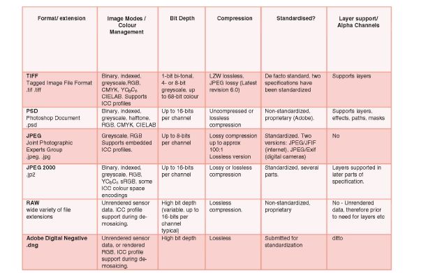
Figure 8.18 Summary of properties of some typical image file formats.

For example, as we have already seen, the choice at image capture between capturing RAW and (most commonly) JPEG files is one about workflow and file size. Further down the imaging chain, an image may be changed to a format more suitable for image editing. Here, the priorities are usually that they are a lossless format and that layers are supported. Some formats also support alpha channels and allow paths to be saved. The selection of a format for output depends on the type of output and the method by which the image is being transmitted, and is a trade-off between file size and quality, but also requires standard formats to ensure that all information (which may include colour profiles and EXIF data) is correctly transmitted with the image. Figure 8.17 illustrates possible workflow in terms of file formats. At the end of this section, Figure 8.18 summarizes some of the important properties of these formats.

Properties of common image file formats

TIFF (Tagged Image File Format)

TIFF is the most commonly used lossless format for imaging and one of the earliest image file formats to be developed. To date it has not been standardized but has become a de facto standard. TIFF is traditionally the format of choice for images used for high-quality and professional output and of course for image archiving, either by photographers or by picture libraries. It should be noted that RAW formats and Adobe DNG files are beginning to be used for personal archives; however, TIFF remains the main lossless format used for images that are optimized and finalized. TIFF is also used in applications in medical imaging and forensics, where image integrity must be maintained, although JPEG 2000 has begun to be adopted in these areas also. TIFF files are usually larger than the raw data itself unless some form of compression has been applied. A point to note is that in the later versions of Photoshop, TIFF files allow an option to compress using JPEG. If this option is selected the file will no longer be lossless. TIFF files support 16-bit colour images and allow layers to be saved without being flattened down, making them a reasonable option as an editing format. The common colour modes are all supported, some of which can include alpha channels. The downside is the large file size and TIFF is not offered as an option in many digital cameras as a result of this, especially since capture using RAW files has now begun to dominate.

PSD (Photoshop Document)

PSD is Photoshop’s proprietary format and is the default option when editing images in Photoshop. It is lossless and allows saving of multiple layers. Each layer contains the same amount of data as the original image; therefore, saving a layer doubles the file size from the original. For this reason, file sizes can become very large and this makes it an unsuitable format for permanent storage. It is therefore better used as an intermediate format, with one of the other formats being used once the image is finished and ready for output.

EPS (Encapsulated Postscript)

This is a standard format that can contain text, vector graphics and bitmap (raster) images. Vector graphics are used in illustration and desktop publishing packages. EPS is used to transfer images and illustrations in postscript language between applications, for example images embedded in page layouts that can be opened in Photoshop. EPS is lossless and provides support for multiple colour spaces, but not alpha channels. The inclusion of all the extra information required to support both types of graphics means that file sizes can be very large. Where it used to be a de facto standard for print, PDF files have largely overtaken in this area.

PDF (Portable Document Format)

PDF files, like EPS, provide support for vector and bitmap graphics and allow page layouts to be transferred between applications and across platforms. PDF also preserves fonts and supports 16-bit images. Again, the extra information results in large file sizes. It was originally released by Adobe Systems and became a de facto standard for the communication of documents containing image and text, as it provides a ‘snapshot’ with limited editing capability of how the document will appear. It has now been standardized and since the free release of the associated Adobe Acrobat reader software has become widely used as a de facto standard for viewing print documents over the Internet.

GIF (Graphics Interchange Format)

GIF images are indexed, resulting in a huge reduction in file size from a standard 24-bit RGB image. GIF was developed and patented as a format for images to be displayed on the Internet, where there is tolerance for the reduction in colours and associated loss in quality to improve file size and transmission. GIF is therefore only really suitable for this purpose.

PNG (Portable Network Graphics)

PNG was developed as a patent-free alternative to GIF for the lossless compression of images on the Web. It supports full 8- and 16-bit RGB images and greyscale as well as indexed images. As a lossless format, compression rates are limited and PNG images are not recognized by all imaging applications, therefore it has not found widespread adoption.

JPEG (Joint Photographic Experts Group)

JPEG is the most commonly used lossy standard. It supports 8-bit RGB, CMYK and greyscale images. When saving from a program such as Photoshop, the user sets the quality setting on a scale of 1–10 or 12 to control file size. In digital cameras there is less control, so the user will normally only be able to select low-, medium- or high-quality settings. JPEG files can be anything from one-tenth to one-hundredth of the size of the uncompressed file, meaning that a much larger number of images can be stored on a camera memory card. However, the large loss in quality makes it an unsuitable format for high-quality output.

JPEG 2000

JPEG 2000 is a more recent standard, also developed by the JPEG committee, with the aim of being more fexible. It allows for 8- and 16-bit colour and greyscale images, supports RGB, CMYK, greyscale and CIELAB colour spaces, and also preserves alpha channels. It allows both lossless and lossy compression, the lossless mode meaning that it will be suitable as an archiving format. The lossy version uses different compression methods from JPEG and aims to provide a slight improvement in quality for the same amount of compression. JPEG 2000 images have begun to be supported by some DSLRs and there are plug-ins for most of the relevant image-processing applications; however, JPEG 2000 images can only be viewed on the Web if the browser has the relevant plug-in.

Adobe Digital Negative

In addition to the Camera RAW plug-in, Adobe are also developing the Digital Negative (.dng) file format, which will be their own version of the RAW file format. Currently it can be used as a method of storing RAW data from cameras into a common RAW format. Eventually, it is intended that it will become a standard RAW format, but we are not at that stage yet, as most cameras do not yet output these files. A few of the high-end professional camera manufacturers do, however, such as Hasselblad, Leica and Ricoh.

Digital colour

Although some early colour systems used additive mixes of red, green and blue, colour in film-based photography is predominantly produced using subtractive mixes of cyan, magenta and yellow (Chapter 1). Both systems are based on trichromatic matching, i.e. colours are created by a combination of different amounts of three pure colour primaries.

Digital input devices and computer displays operate using additive RGB colour. At the print stage, cyan, magenta and yellow dyes are used, usually with black (the key) added to account for deficiencies in the dyes and improve the tonal range. In modern printers, more than three colours may be used (six- or even eight-ink printers are now available and the very latest models by Canon and Hewlett Packard use 10 or 12 inks to increase the colour gamut), although they are still based on a CMY(K) system.

An individual pixel will therefore usually be defined by three (or four, in the case of CMYK) numbers specifying the amount of each primary. These numbers are coordinates in a colour space. A colour space provides a three-dimensional (usually) model into which all possible colours may be mapped (see Figure 8.19). Colour spaces allow us to visualize colours and their relationship to each other (see Chapter 1). RGB and CMYK are two broad classes of colour space, but there are a range of others, as already encountered, some of which are much more specific and defined than others (see next section). The colour space defines the axes of the coordinate system and, within this, colour gamuts of devices and materials may then be mapped; these are the limits to the range of colours capable of being reproduced.

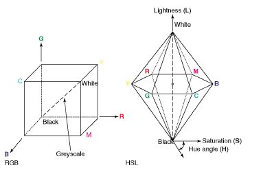
Figure 8.19 RGB and HSL. Colour spaces are multi-dimensional coordinate systems in which colours may be mapped: R (red), G (green), B (blue), M (magenta), C (cyan) and Y (yellow).

The reproduction of colour in digital imaging is therefore more complex than that in traditional silver halide imaging, because both additive and subtractive systems are used at different stages in the imaging chain. Each device or material in the imaging chain will have a different set of primaries. This is one of the major sources of variability in colour reproduction. Additionally, colour appearance is influenced by how devices are set up and by the viewing conditions. All these factors must be taken into account to ensure satisfactory colour. As an image moves through the digital imaging chain, it is transformed between colour spaces and between devices with gamuts of different sizes and shapes: this is the main problem with colour in digital imaging. The process of ensuring that colours are matched to achieve reasonably accurate colour and tone reproduction requires colour management.

Colour spaces

Colour spaces may be broadly divided into two categories: device-dependent and device-independent spaces. Device-dependent spaces are native to input or output devices. Colours specified in a device-dependent space are specific to that device, they are not absolute. Device-independent colour spaces specify colour in absolute terms. A pixel specified in a device-independent colour space should appear the same, regardless of the device on which it is reproduced.

Device-dependent spaces are defined predominantly by the primaries of a particular device, but also by the characteristics of the device, based upon how it has been calibrated. This means, for example, that a pixel with RGB values of 100, 25 and 255, when displayed on two monitors from different manufacturers, will probably be displayed as two different colours, because in general the RGB primaries of the two devices will be different. Additionally, as seen in Chapter 1, the colours in output images are also affected by the viewing conditions. Even two devices of the same model from the same manufacturer will produce two different colours if set up differently (see Figure 8.20). RGB and CMYK are generally device dependent, although there are some standardized RGB spaces that are device independent under certain conditions (sRGB is an example). These spaces have a direct relationship to CIE colorimetric values, meaning that the transforms required to convert from, for example sRGB to CIELAB, are known.

Device-independent colour spaces are derived from CIEXYZ colorimetry, i.e. they are based on the response of the human visual system. CIELAB and CIELUV are examples. sRGB is actually a device calibrated colour space, specified for images displayed on a cathode ray tube

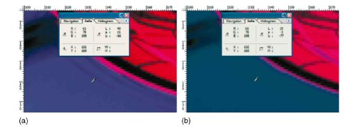
Figure 8.20 Pixel values, when specified in device-dependent colour spaces, will appear as different colours on different devices.

(CRT) monitor; if the monitor and viewing environment are correctly set up, then the colours will be absolute and it acts as a device-independent colour space.

A number of common colour spaces separate colour information from tonal information, having a single coordinate representing tone, which can be useful for various reasons. Examples include hue, saturation and lightness (HSL) (see Figure 8.19) and CIELAB (see page 16); in both cases the Lightness channel (L) represents tone. In such cases, often only a slice of the colour space may be displayed for clarity; the colour coordinates will be mapped in two dimensions at a single lightness value, as if looking down the lightness axis, or at a maximum chroma regardless of lightness. Two-dimensional CIELAB and CIE xy diagrams are examples commonly used in colour management, particularly for the comparison of device gamuts and the identifcation of out-of-gamut colours.

Colour gamuts

The colour gamut of a particular device defines the possible range of colours that the device can produce under particular conditions. Colour gamuts are usually displayed for comparison in a device-independent colour space such as CIELAB or CIE xy. Because of the different technologies used in producing colour, it is highly unlikely that the gamuts of two devices will exactly coincide. This is known as gamut mismatch (see Figure 8.21). In this case, some colours are within the gamut of one device but lie outside that of the other; these colours tend to be the more saturated ones. A decision needs to be made about how to deal with these out-of-gamut colours. This is achieved using rendering intents in an ICC colour management system. They may be clipped to the boundary of the smaller gamut, for example, leaving all other colours unchanged; however, this means that the relationships between colours will be altered and that many pixel values may become the same colour, which can result in posterization. Alternatively, gamut compression may be implemented, where all colours are shifted inwards, becoming less saturated, but maintaining the relative differences between the colours and so achieving a more natural result.

Figure 8.21 Gamut mismatch. The gamuts of different devices are often different shapes and sizes, leading to colours that are out of gamut for one device or the other. In this example, the gamut of an image captured in the Adobe RGB (1998) colour space is wider than the gamut of a CRT display.

Colour management systems

A colour management system is a collection of hardware and software which works with imaging applications and the computer operating system to communicate and match colours through the imaging chain. Colour management reconciles differences between the colour spaces of each device and allows us to produce consistent colours. The aim of the colour management system is to convert colour values successfully between the different colour spaces so that colours appear the same or acceptably similar, at each stage in the imaging chain. To do this the colours have to first be specified.

The conversion from the colour space of one device to the colour space of another is complicated. As already discussed, input and output devices have their own colour spaces; therefore, colours are not specified in absolute terms. An analogy is that the two devices speak different languages: a word in one language will not have the same meaning in another language unless it is translated; additionally, words in one language may not have a direct translation in the other language. The colour management system acts as the translator.

ICC colour management

The International Color Consortium (ICC) is made up of over 70 members from all areas of the imaging and computing industries. Their aim is to promote the adoption of universal methods of colour management. To this end, they have developed a standardized colour management architecture based on the use of colour profiles. More information about the ICC and their work can be found at www.color.org. ICC colour management systems have four main components:

1. Profile connection space (PCS). The PCS is a device-independent colour space, generally CIEXYZ or CIELAB, which is used as a software ‘hub’, into which all colours are transformed into and out of. Continuing with the language analogy, the PCS is a central language and all device languages are translated into the PCS and back again: generally there is no direct translation from one device to another (although there is the option for this in some specialist applications in the latest ICC specification, it is rarely used).

2. ICC profiles. A profile is a data file containing information about the colour reproduction capabilities of a device, such as a scanner, a digital camera, a monitor or a printer. There are also a number of intermediate profiles, which are not specific to a device but to a colour space, usually a working colour space. The profling of a device is achieved by calibration and characterization. These processes produce the information necessary for mapping colours between the device colour space and the PCS. This information is carried within the profile in the form of either matrix transforms (which are applied to each set of pixel values to find the values in the new colour space) or a look-up table (LUT). The ICC provides a standard format for these profile files, which allows them to be used by different devices and across different platforms and applications. This means that an image can be embedded with the profile from its capture device and when imported into any computer running an ICC colour managed system, the colours should be correctly reproduced. Images can also be assigned profiles, or converted between profiles (see later section on using profiles).

3. Colour management module (CMM). The colour management module is the software ‘engine’ which performs all the calculations for colour conversions. The CMM is separate from the imaging application and is part of the operating system. There are a number of standard ones for both Mac and PC, which can be selected through the system colour management settings.

4. Rendering intents. Rendering intents define what happens to colours when they are ‘out of gamut’, i.e. outside the gamut of the output device. The rendering intent is selected by the user at a point when an image is to be converted between two colour spaces, for example when converting between profiles, or when sending an RGB image to print. There are four ICC specified rendering intents, optimized for different imaging situations. These are: perceptual, saturation, media relative colorimetric and absolute colorimetric. Generally, for most purposes, you will only use the perceptual and relative colorimetric intents; the other two are optimized for saturated graphics and for proofng in a printing press environment respectively and are less likely to give a satisfactory result for everyday imaging.

5. On a simple level, the perceptual intent will ft the out-of-gamut colours inside the destination gamut by compressing and shifting all colours. This means that all colours will change slightly but the relative differences between colours will remain the same, providing a more pleasing image. The intent is most suitable for images with many out-of-gamut colours. The media relative colorimetric intent clips out-of-gamut colours to the gamut boundary. All in-gamut colours are shifted relative to the white point of the output medium. It will again produce pleasing results but is better with images with fewer out-of-gamut colours.

6. Previewing when converting or printing will allow you to select the best one for your image.

Fundamental concepts

ICC colour management requires a bit of work in setting up and understanding how it works, but provides an elegant solution to a complicated problem. In summary:

• Profiles provide information about colour spaces. The information in the file allows correct conversion of colour values between the particular colour space and the PCS.
• Each conversion between profiles requires a source and a destination profile.
• The image is assumed to have a profile associated with it at all stages in the imaging chain. The profile may be that of an input or output device, or a working space profile.
• If an image enters the workspace without a profile, then a profile may be assigned to it. This does not alter the underlying pixel values.
• Images may be converted between profiles at any point in the imaging chain. Conversion will change the image values, but should not alter the image appearance.
• When converting the image, the user selects a rendering intent, which specifes how out-of-gamut colours will be dealt with.
• Only convert between colour spaces when actually necessary, to minimize colour artefacts.

Profling: calibration and characterization of devices

Fundamental to all colour management is knowledge about the devices and materials being used. Without this information, it is impossible to perform the conversions between colour spaces and ensure correct colour reproduction. This requires two processes.

Calibration

Calibration is twofold: there is the initial set-up of the devices in an imaging chain to a required state, followed by ongoing calibration to return them to this state. Initial calibration will normally involve setting a number of characteristics that will control device contrast, tone reproduction and colour gamut. The methods used will vary from device to device. As shown in Chapter 7, calibration of a monitor usually involves setting of brightness and contrast controls, colour temperature and sometimes individual balancing of the RGB controls. Calibration of a printer involves selection of inks and paper, and setting of a gamma value, which ensures that all tones from shadows to highlights are correctly spaced.

It is important to remember that a profile is created for a device when it is in a particular calibrated state. If the device changes from that state, the profile will no longer be accurate. For this reason, ongoing calibration is an important aspect of colour management. This also means that, each time a change is made at the print stage, for example a different ink set or a different type of paper is used, the system must be recalibrated and a profile created for that particular condition; in the end you will need profiles for each paper surface that you use.

Characterization

Following the initial calibration, characterization involves the reproduction of a set of standard colours by the device being profiled. For a camera or scanner, a standard test chart is captured. For a printer the test chart is printed. For a monitor a standard set of colour patches is displayed on screen, usually produced automatically by the software of the profling device. The colours produced by the device are then measured colorimetrically and their values compared with the original values. From this information the profling device software then creates the profile.

There are a number of profling devices available. These vary in complexity and price. Generally the devices will perform both calibration and characterization. Calibration devices for monitors (see page 189) tend to be reasonably affordable; therefore, at the very least, try and invest in one. The display is the most important device in terms of colour management, as most of your ‘work’ on the images will be performed on screen and displays need to be calibrated regularly. Printer calibration tools tend to be more at the professional end of the market, and therefore more expensive. Often, profling devices will be multi-functional and come with bundled software, which allows you to profile all the devices in your imaging chain. If you are serious about colour management, you need to consider this, but do your research first and ensure that you get proper training as part of the package.

Although, theoretically, all the devices in the imaging chain should be profiled, it is possible to get away without profling input devices. Scanners tend to be very stable in their colour reproduction. If a scanner is to be profiled, it must be profiled for each type of material being scanned, e.g. each film type. Often manufacturer profiles will be provided with the scanner software for a range of different materials. Because scanning is a relatively slow process, where the image is often viewed and adjusted on a large preview screen, these may well suffce.

Cameras are a different issue. Profling a digital camera involves photographing a test chart under even illumination. The profile created will only be really accurate under the same illumination. The range of different shooting conditions that you will usually encounter means that a camera profile created in this way is not going to be particularly useful or meaningful (note, however, that under scientific conditions, where images are all being shot in a very controlled manner, a profile is essential).

Generally, therefore, you will simply set the capture colour space using one of the options available in the camera software. This will capture your camera into one of the standard workspaces, sRGB or Adobe RGB (1998) (see the section on capture workflow, earlier in this chapter).

Setting colour preferences in Photoshop

This is an important stage in the process of colour management. It does not need to be done each time the application is opened up, but should be done before you start. The colour preferences define the overall default behaviour of Photoshop. To set the preferences go to the Edit menu and select Color Settings. A window will open up with a number of default settings. These define the working colour spaces and colour management policies. The default RGB colour space is generally sRGB. As stated before, sRGB is a semi-standardized colour space optimized for multimedia images. Unless all of your images are to be viewed on screen, it is suggested that you change this to Adobe RGB (1998), because its larger gamut is more likely to match the range of printers you may use. The CMYK colour space defines the gamut of the ink set you are most likely to encounter if your images are published in print. This should be set according to your geographical location. If in Europe, select one of the European sets, if in the United States, select one of the US sets, etc. It is suggested that the remaining settings are set as in Figure 8.22. These ensure that if an image enters the workspace with a profile, then that profile will be preserved and there will be no automatic conversion. Additionally, if the image has a corrupted or missing profile, Photoshop will fag this up, allowing you to decide which profile you will assign to it.

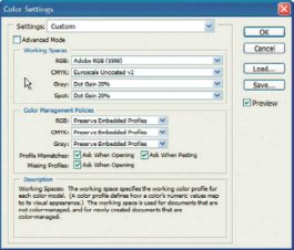
Figure 8.22 Colour settings in Photoshop.

Dealing with profiles: assigning and converting

Images will often come into the application workspace with an embedded profile. Camera software, for example, may automatically embed the profile in the image, its contents providing the colour management system with the information required to correctly interpret the image pixel values.

Figure 8.23 Options when assigning a profile.

There will be times, however, when images enter the workspace without a profile for some reason, or with a corrupted profile. If the colour settings in Photoshop are set as suggested above, the application should then fag this up. It is at this point that it is useful to assign a profile. To do this, go to Image > Mode > Assign Profile. A window will pop up as shown in Figure 8.23. The profile menu lists all the profiles on the system, including workspace profiles, manufacturers’ profiles and device profiles. Assigning a profile allows the user to test out different profiles, to identify the one that best displays the image. Assigning will not convert the underlying pixel values, but may change image appearance; it is like viewing the image through a coloured filter (see Figure 8.24).

At certain points in the imaging chain, it may also be necessary to convert between profiles. This is really a conversion between two colour spaces and therefore requires a source and destination profile. The source profile will be the one either embedded in or assigned to the image. The destination profile will be the one you are converting it to. To convert an image, go to Image > Mode > Convert to Profile and a window will pop up similar to the one in Figure 8.25. You must specify the output profile, the CMM (the ‘Engine’) and the rendering intent.

Conversion involves a non-reversible change in the image values; however, the change in image appearance should be minimal. The colour values in the image are being converted into the closest possible values in the destination space. Almost inevitably, some colours will be out of gamut, so some values will be slightly different, i.e. some loss will occur.

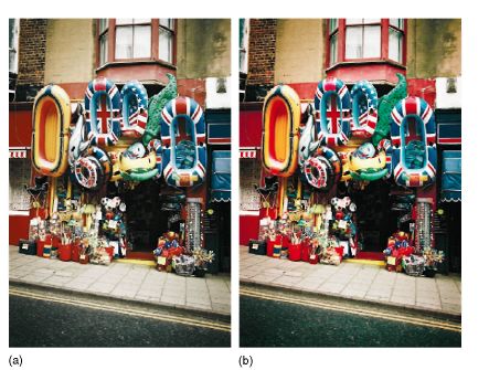
Figure 8.24 Assigning different profiles. The image colours change when the image is assigned. (a) Pro-Photo RGB. (b) sRGB.

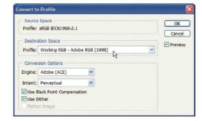
Figure 8.25 Converting between profiles. The user must specify source and destination profiles, the CMM and the rendering intent.

It is therefore important that you do not convert images more often than is necessary.

Colour management using Photoshop

The following provides some guidelines for implementation of profiled colour management in Photoshop. Some aspects may vary depending upon the version of Photoshop being used, so also check the help files for your version. Refer to the previous sections for details on the methods at each stage. It assumes that you are working with RGB images at input.

1. Set Photoshop colour preferences (this only needs to be done once).

2. Profile your devices. At the very least, profile your display. If you do not have access to a profling device, use visual calibrator software such as Adobe Gamma (Windows) or Monitor Calibrator (MacOS). Ensure that the correct profile is being used by the display.

3. Importing images:

a) When an image is imported into Photoshop and has a correctly embedded source profile, preserve the profile (if you have set up Photoshop as shown, you will not need to alter anything).

b) If an image is imported without a profile, or with a corrupted profile, assign a profile to it. You may assign a number of different profiles, to find the one producing the most satisfactory colours, or choose to assign your working space RGB profile.

4. Editing images: it is common nowadays to work in an RGB colour space, only converting to CMYK at the last minute. This is because images are not always going to be printed, or it may be that they are to be published on the Web as well, so an RGB version is needed. CMYK gamuts are always smaller than RGB, therefore by using an RGB space you will have more colours available at the all-important editing stage. It can be useful to convert the image into a standardized RGB space, so you may choose before editing to convert to your working RGB colour space using the Convert to Profile command.

5. Soft-proof when printing images: soft-proofng allows you to display your image colours on screen so that they appear as close as possible to the way they will look when printed, to allow for last-minute adjustments. Your display must be calibrated and profiled and the printer must be profiled for the paper and inks that you are using. To set up soft-proof, go to View > Proof Setup > Custom and in the window that pops up, set your printer profile and required rendering intent. To view the soft proof, go to the View menu and select Proof Colors.

6. The final colour conversion when printing can be performed within Photoshop or by the printer software, so needs to be enabled in only one of them. Otherwise, the conversions will be performed twice, with unpredictable results. The suggested process is as follows:

a) Open up the print command window using File > Print with Preview (see Figure 8.26). Ensure that ‘colour management’ is selected in the top left drop-down menu, as shown. ‘Document’ should be selected as source space as shown, and the correct printer profile and required rendering intent should be selected in print space. Black point compensation ensures that the black point will remain black in the printed image, so unless you have very good reason, you should leave this checked.

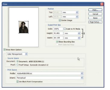
Figure 8.26 Print with preview window in Photoshop.

b) Set the page set-up parameters in the right-hand side of the window. The position of the printed image will appear in the pane on the left. The page set-up button allows you to alter the orientation of the paper and the paper size. Once completed, press the print button.

c) A second print window will open up. Ensure that colour management is turned off in this window, as this is the device software window. This will make certain that colour management is only performed by Photoshop.

Image processing

There are a huge range of processes that may be applied to a digital image to optimize, enhance or manipulate the results. Equally, there are many types of software to achieve this, from relatively simple easy-to-use applications bundled with devices for the consumer, to high-end professional applications such as Adobe Photoshop. It is beyond the scope of this book to cover the full range of image processing, or to delve into the complexities of the applications. The Adobe Photoshop workspace and various tools are dealt with in more detail in Langford’s Basic Photography. There are, however, a number of processes that are common to most image-processing software packages and will be used time and again in adjusting images; it is useful to understand these, in particular the more professional tools. The following sections concentrate on these key processes and how they fit into an image-processing workflow.

Image-processing techniques are fundamentally numerical manipulations of the image data and many operations are relatively simple. There are often multiple methods to achieve the same effect. Image processing is applied in some form at all stages in the imaging chain (Figure 8.27).

The operations may be applied automatically at a device level, for example by the firmware in a digital camera, with no control by the user; they may also be applied as a result of scanner, camera or printer software responding to user settings, and some functions are applied ‘behind the scenes’, such as the gamma correction function applied to image values by the video graphics card in a computer monitor to ensure that image tones are displayed correctly. The highest level of user control is achieved in a dedicated application such as Adobe Photoshop or Image J.

Because the image is being processed throughout the image chain, image values may be repeatedly changed, redistributed, rounded up or down, and it is easy for image artefacts to appear as a result of this. Indeed, some image-processing operations are applied automatically to correct for the artefacts introduced by other operations, for example image sharpening in the camera, which is applied to counteract the softening of the image caused by noise removal algorithms and interpolation. When the aim is to produce professional-quality photographic images, the approach to image editing has to be ‘less is more’, avoiding overapplication of any method, applying by trial and error, using layers and history to allow correction of mistakes, with care taken in the order of application and an understanding of why a particular process is being carried out.

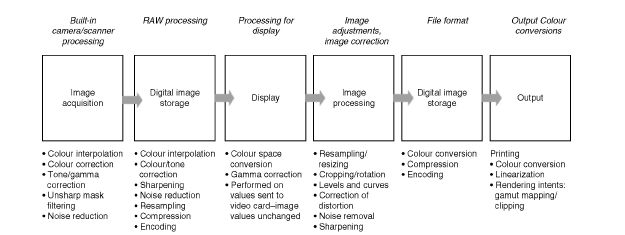
Figure 8.27 Image processing through the imaging chain.

Using layers

Making image adjustments using layers allows image-processing operations to be applied and the results seen, without being finalized. A background layer contains the unchanged image information, and instead of changing this original information, for example, a tonal adjustment can be applied to all or part of the image in an adjustment layer. While the layer is on top of the background and switched ‘on’ the adjustment can be seen on the image. If an adjustment is no longer required, the layer can be discarded. Selections can also be made from the image and copied into layers, meaning that adjustments may be performed to just that part of the image, or that copied part can be imported into another image.

Layers can be grouped, their order can be changed to produce different effects, their opacity changed to alter the degree by which they affect the image and they can be blended into each other using a huge range of blending modes. Layers can also be made partially transparent, using gradients, meaning that in some areas the lower layers or the original image state will show through. Working with layers allows image editing to become an extremely fuid process, with the opportunity to go back easily and correct, change or cancel operations already performed. When the editing process is finished, the layers are flattened down and the effects are then permanent.

Image adjustment and restoration techniques

Image adjustments are a basic set of operations applied to images post-capture to optimize quality and image characteristics, possibly for a specific output. These operations can also be applied in the capture device (if scanning) after previewing the image, or in RAW processing and Lightroom software. Image adjustments include cropping, rotation, resizing, tone and colour adjustments. Note that image resizing may be applied without resampling to display image dimensions at a particular output resolution – this does not change the number of pixels in the image and does not count as an image adjustment.

Image correction or restoration techniques correct for problems at capture. These can be globally applied or may be more local adjustments, i.e. applied only to certain selected pixels, or applied to different pixels by different amounts. Image corrections include correction of geometric distortion, sharpening, noise removal, localized colour and tonal correction, and restoration of damaged image areas. It is not possible to cover all the detailed methods available in all the different software applications to implement these operations; however, some general principles are covered in the next few sections, along with the effects of overapplication.

Image-processing workflow

The details of how adjustments are achieved vary between applications, but they have the same purpose; therefore, a basic workflow can be defined. You may find alternative workflows work better for you, depending upon the tools that you use; what is important is that you think about why you are performing a particular operation at a particular stage and what the implications are of doing things in that order. It will probably require a good degree of trial and error. A typical workflow might be as follows:

1. Image opened, colour profile identified/assigned. In a colour profiled workflow, the profile associated with the image will be applied when the image is opened (see later section on ICC colour management). This ensures that the image colours are accurately displayed on screen.

2. Image resized. This is the first of a number of resampling operations. If the image is to be resized down, then it makes sense to perform it early in the workflow, to reduce the amount of time that other processes may take.

3. Cropping, rotation, correction of distortion. These are all spatial operations also involving resampling and interpolation and should be performed early in the workflow, allowing you to frame the image and decide which parts of the image content are important or less relevant.

4. Setting colour temperature. This applies to Camera RAW and Lightroom, as both are applications dealing with captured images, and involves an adjustment of the white point of the image, to achieve correct neutrals. This should be performed before other tone or colour correction, as it will alter the overall colour balance of the image.

5. Global tone correction. This should be applied as early as possible, as it will balance the overall brightness and contrast of the image and may alter the colour balance of the image. There are a range of exposure, contrast and brightness tools available in applications such as Photoshop, Lightroom and Camera RAW. The professional tools, allowing the highest level of user control, especially over clipping of highlights or shadows, are based upon levels or curves adjustments, which are covered later in this chapter.

6. Global colour correction. After tone correction, colours may be corrected in a number of ways. Global corrections are usually applied to remove colour casts from the image. If across the whole range from shadows to highlights, then this is easier, changing a single or several colour channels, and the simpler tools, such as ‘photo filter’ in Photoshop, will be successful. More commonly there will be just part of the brightness range, such as the highlights that will need correcting, in which case altering the curves across the three channels affords more control. There are other simple tools such as colour balance in Photoshop, and the saturation tool. Care should be taken with these, as they can produce rather crude results and may result in an increase in colours that are out of gamut (i.e. they are outside the colour gamuts of some or all of the output devices and therefore cannot be reproduced accurately).

7. Noise removal. There are a range of filters created specifically for removal of various types of noise. Applying them globally may remove unwanted dust and scratches, but care should be taken as they often result in softening of edges. Because of this, it is often better to apply them in Photoshop if possible, as you have a greater range of filters at your disposal and you can use layers to fine-tune the result.

8. Localized image restoration. These are the corrections to areas that the noise removal filters did not work on. They usually involve careful use of some of the specially designed restoration tools in Photoshop, such as the healing brush or the patch tool. In other packages this may involve using some form of paint tool.

9. Local tone and colour corrections. These are better carried out after correction for dust and scratches. They involve the selection of specific areas of the image, followed by correction as before.

10. Sharpening. This is also a filtering process. Again, there are a larger range of sharpening tools available in Photoshop and a greater degree of control afforded using layers.

Image resizing, cropping, rotation and correction of distortion

These are resampling operations that involve the movement or deletion of pixels or the introduction of new pixels. They also involve interpolation, which is the calculation of new pixel values based on the values of their neighbours. Cropping alone involves dropping pixels without interpolation, but is often combined with resizing or rotation. Depending upon where in the imaging chain these operations are performed, the interpolation method may be predefined and optimized for a particular device, or may be something that the user selects. The main methods are as follows:

• Nearest neighbour interpolation is the simplest method, in which the new pixel value is allocated based on the value of the pixel closest to it.
• Bilinear interpolation involves the calculation of the new pixel value by taking an average of its four closest neighbours and therefore produces significantly better results than nearest neighbour sampling.
• Bicubic interpolation involves a complicated calculation involving 16 of the pixel’s neighbouring values. The slowest method also produces the best results with fewer visible artefacts and therefore is the best technique for maintaining image quality.

Interpolation artefacts and workflow considerations

In terms of workflow, these operations are usually the first to be applied to the image, as it makes sense to decide on image size and content before applying colour or tonal corrections to pixels that might not exist after resampling has been applied. Because interpolation involves the calculation of missing pixel values, it inevitably introduces a loss in quality.

Nearest neighbour interpolation is a rather crude method of allocating pixel values and produces an effective magnification of pixels as well as a jagged effect on diagonals (see Figure 8.28(b)) - this is actually an aliasing artefact (see Chapter 6) as a result of the edge

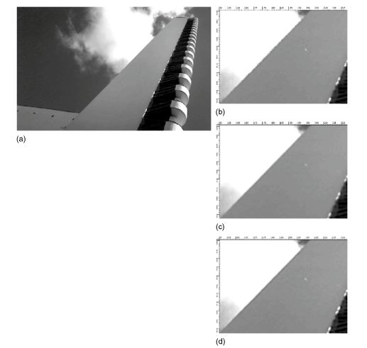
Figure 8.28 Interpolation artefacts. (a) Original image. A small version of this image is resampled to four times its original size using various interpolation methods. (b) Nearest neighbour interpolation shows staircasing on diagonals. (c) Bilinear interpolation produces significant blurring on edges. (d) There is some blurring with bicubic interpolation, but it clearly produces the best results of the three. Image© Elizabeth Allen

being undersampled. Both are so severe visually that it is hard to see when the method would be selected as an option, especially when the other methods produce much more pleasing results.

Bilinear and bicubic interpolation methods, however, involve a process of averaging surrounding values. Averaging processes produce another type of artefact, the blurring of edges and fine detail (see Figure 8.28(c, d)). This again is more severe the more that the interpolation is applied. Because bicubic interpolation uses more values in the calculation of the average, the smoothing effect is not as pronounced as it is with bilinear.

Repeated application of any of these operations simply compounds the loss in image quality, as interpolated values are calculated from interpolated values, becoming less and less accurate. For this reason, these operations are best applied in one go wherever possible. Therefore, if an image requires rotation by an arbitrary amount, find the exact amount by trial and error and then apply it in one application rather than repeating small amounts of rotation incrementally. Equally, if an image requires both cropping and perspective correction, perform both in a combined single operation to maintain maximum image quality.

Tone and colour corrections

These are methods for redistributing values across the tonal range in one or more channels to improve the apparent brightness or contrast of the image, to bring out detail in the shadows or the highlights or to correct a colour cast. These corrections are applied extensively throughout the imaging chain, to correct for the effects of the tone or gamut limitations of devices, or, for creative effect, to change the mood or lighting in the image.

Brightness and contrast controls

The simplest methods of tonal correction are the basic brightness and contrast settings found in most image-processing interfaces, which involve the movement of a slider or a number input by the user (Figure 8.29). These are not really professional tools, and are often simple additions or subtractions of the same amount to all pixel values, or multiplication or division by the same amount, and mean that there is relatively limited control over the process. With even less control are the ‘auto’ brightness and contrast tools, which are simply applied to the image and allow the user no control whatsoever, often resulting in posterization as a result of lost pixel values.

Figure 8.29 Global brightness and contrast controlled by simple sliders.

Adjustments using levels

Levels adjustments use the image histogram and allow the user interactive control over the distribution of tones in shadows, midtones and highlights. A simple technique for improving the tonal range is illustrated in Figure 8.30, where the histogram of a low-contrast image is improved by (1) sliding the shadow control to the edge of the left-hand side of the range of tonal values, (2) sliding the highlight slider to the right-hand side of the range and (3) sliding the midtone slider to adjust overall image brightness.

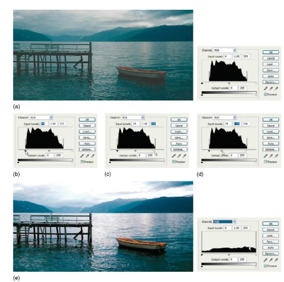
Figure 8.30 Levels adjustment to improve tone and contrast. (a) Original image and its histogram. (b) Shadow control levels adjustment. (c) Highlight control levels adjustment. (d) Midtone adjustment. (e) Final image and histogram. Image © Elizabeth Allen

The same process can be applied separately to the channels in a colour image. Altering the shadow and highlight controls of all three channels will improve the overall image contrast. Altering the midtone sliders by different amounts will alter the overall colour balance of the image.

Curves

These are manipulations of the tonal range using the transfer curve of the image, which is a simple mapping function allowing very precise control over specific parts of the tonal range. The curve shows output (vertical axis) plotted against input (horizontal axis). Shadows are usually at the bottom left and highlights at the top right. Before any editing it is displayed as a straight line at 45° (Figure 8.31(a)). As with levels it is possible to display the combined curve, in this case RGB, or the curves of individual colour channels.

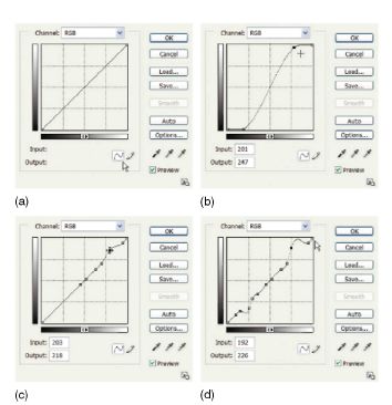
Figure 8.31 (a) Initial curve. (b) Global contrast enhancement. (c) Localized correction. (d) Overcorrection as a result of too many selection points.

The curve can be manipulated by selecting an area and moving it. If the curve is at an angle steeper than 45°, and if this is applied globally to the full range of the curve as shown in Figure 8.31(b), then the contrast of the output image will be higher than that of the input. If the curve is not as steep as 45° then contrast will be lowered.

Multiple points can be selected to ‘peg down’ areas of the curve, allowing the effect to be localized to a specific range of values. The more points that are added around a point in question, the more localized the control will be. Again, a steeper curve will indicate an increase in contrast and shallower a decrease (Figure 8.31(c, d)). Using a larger number of selected points allows a high degree of local control; however, it is important to keep on checking the effect on the image, as too many ‘wiggles’ are not necessarily a good thing – in the top part of the curve in Figure 8.31(d), the distinctive bump actually indicates a reversal of tones.

Using curves to correct a colour cast

This is where having an understanding of basic colour theory is useful. Because the image is made up of only three (or four) colour channels, then most colour casts can be corrected by using one of these. Look at the image and identify what the main hue of the colour cast is. From this, you can work out which colour channel to correct. Both the primary and its complementary colour will be corrected by the same colour channel:

Colour cast	Correction channel
Red or Cyan	Red
Green or Magenta	Green
Blue or Yellow	Blue

Artefacts as a result of tone or colour corrections

As with all image processes, overzealous application of any of these methods can result in certain unwanted effects in the image. Obvious casts may be introduced as a result of overcorrecting one colour channel compared to the others. Overexpansion of the tonal range in any part can

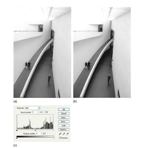
Figure 8.32 (a) Original image. (b) Posterized image. (c) Histogram. Image © Elizabeth Allen

result in missing values and a posterized image (see Figure 8.32). Lost levels cannot be retrieved without undoing the operation, and therefore should be avoided by applying corrections in a more moderate way and by using 16-bit images wherever possible. Another possible effect is the clipping of values at either end of the range, which will result in loss of shadow detail and burning out of highlights, and will show as a peak at either end of the histogram.

Filtering operations

Both noise removal and image sharpening are generally applied using filtering. Spatial filtering techniques are neighbourhood operations, where the output pixel value is defined as some combination or selection from the neighbourhood of values around the input value. The methods discussed here are limited to the filters used for correcting images, not the large range of special effects creative filters in the filter menu of image-editing software such as Adobe Photoshop.

The filter (or mask) is simply a range of values which are placed over the neighbourhood around the input pixel. In linear filtering the values in the mask are multiplied by the values in

Figure 8.33 The process of linear filtering. The mask values are multiplied with the neighbourhood pixel values and the results summed to produce the output value.

Figure 8.34 A small section of an image and corresponding pixel values is filtered by a 3 × 3 blurring filter. The noisy pixel in the top left of the image is removed using this filter, although the diagonal edge at bottom right is also blurred.

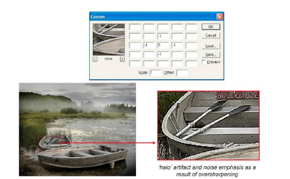
Figure 8.35 An illustration of linear filtering in Adobe Photoshop using the ‘custom’ filter. A high central value and surrounding low negative values in the filter can be used in a sharpening filter.

the image at neighbourhood at the same point and the result is added together (Figure 8.33) and sometimes averaged. Blurring and sharpening filters are generally of this type (Figure 8.34). It is possible to see the process of linear filtering (mathematically this is known as convolution) in Adobe Photoshop by going to the filter menu and selecting ‘custom’, which allows you to select the values to input into the filter yourself. This is illustrated in Figure 8.35.

Non-linear filters simply use the mask to select the neighbourhood. Instead of multiplying the neighbourhood with mask values, the selected pixels are sorted and a value from the neighbourhood output, depending on the operation being applied. The median filter is an example, where the median value is output, eliminating very high or low values in the neighbourhood, making it very successful for noise removal.

Noise removal

There are a range of both linear and non-linear filters available for removing different types of noise and specially adapted versions of these may also be built in to the software of capture devices. Functions such as digital ICE™ for suppression of dust and scratches in some scanner software are based on adaptive filtering methods. The linear versions of noise removal filters tend to be blurring filters, and result in edges being softened; therefore, care must be taken when applying them (Figure 8.36). Non-linear filters such as the median filter, or the ‘dust and speckles’ filter in Photoshop, are better at preserving edges, but can result in posterization if applied too heavily.

Sharpening

Sharpening tends to be applied using linear filters. Sharpening filters emphasize edges, but may also emphasize noise, which is why sharpening is better performed after noise removal.

Figure 8.36 Filtering artefacts. (a) Original image. (b) Noise removal filters can cause blurring and posterization, and oversharpening can cause a halo effect at the edges. (c) This halo effect is clearly shown in a magnified section of the sharpened image.

The unsharp mask is a filter based upon a method used in the darkroom in traditional photographic imaging, where a blurred version of the image is subtracted from a boosted version of the original, producing enhanced edges. This can be successful, but again care must be taken not to oversharpen. As well as boosting noise, oversharpening produces a characteristic ‘overshoot’ at edges, similar to adjacency effects, known as a halo artefact (Figure 8.36(c)). For this reason sharpening is better performed using layers, where the effect can be carefully controlled.