This chapter covers

• Programming a simulator for multiple qubits using the QuTiP Python package and tensor products
• Recognizing the proof that quantum mechanics is consistent with our observations of the universe by simulating experimental results

In the previous chapter, we learned about nonlocal games and how we can use them to validate our understanding of quantum mechanics. We also learned how to represent states of multiple qubits and what entanglement is.

In this chapter, we will dive into a new Python package called QuTiP that will allow us to program quantum systems faster and has some cool built-in features for simulating quantum mechanics. Then we’ll learn how to use QuTiP to program a simulator for multiple qubits and see how that changes (or doesn’t!) the three main tasks for our qubits: state preparations, operations, and measurement. This will let us finish the implementation of the CHSH game from chapter 4!

5.1 Quantum objects in QuTiP

QuTiP (Quantum Toolbox in Python, www.qutip.org) is a particularly useful package that provides built-in support for representing states and measurements as bras and kets, respectively, and for building matrices to represent quantum operations. Just as np.array is at the core of NumPy, all of our use of QuTiP will center around the Qobj class (short for quantum object). This class encapsulates vectors and matrices, providing additional metadata and useful methods that will make it easier for us to improve our simulator. Figure 5.1 shows an example of creating a Qobj from a vector, where it keeps track of some metadata:

• data holds the array representing the Qobj.

• dims is the size of our quantum register. We can think of it as a way of keeping track of how we record the qubits we are dealing with.

• shape keeps the dimension of the original object we used to make the Qobj. It is similar to the np.shape attribute.

• type is what the Qobj represents (a state = ket, a measurement = bra, or an operator = oper).

Figure 5.1 Properties of the Qobj class in the QuTiP Python package. Here we can see things like the type and dims properties that help both us and the package keep track of metadata about our quantum objects.

Let’s try importing QuTiP and asking it for the Hadamard operation; see listing 5.1.

Note Make sure as you run things that you are in the right conda env; for more information, see appendix A.

Listing 5.1 QuTiP’s representation of the Hadamard operation

>>> from qutip.qip.operations import hadamard_transform
>>> H = hadamard_transform()
>>> H
Quantum object: dims = [[2], [2]], shape = (2, 2), type = oper, isherm = True
Qobj data =
[[ 0.70710678  0.70710678]
 [ 0.70710678 -0.70710678]]

Note that QuTiP prints out some diagnostic information about each Qobj instance along with the data itself. Here, for instance, type = oper tells us that H represents an operator (a more formal term for the matrices we’ve seen so far) along with some information about the dimensions of the operator represented by H. Finally, the isherm = True output tells us that H is an example of a special kind of matrix called a Hermitian operator.

We can make new instances of Qobj in much the same way we made NumPy arrays, by passing in Python lists to the Qobj initializer.

Listing 5.2 Making a Qobj from a vector representing a qubit state

>>> import qutip as qt
>>> ket0 = qt.Qobj([[1], [0]])                                   ❶
>>> ket0
Quantum object: dims = [[2], [1]], shape = (2, 1), type = ket    ❷
Qobj data =
[[1.]
 [0.]]

❶ One key difference between creating Qobj instances and arrays is that when we create Qobj instances, we always need two levels of lists. The outer list is a list of rows in the new Qobj instance.

❷ QuTiP prints some metadata about the size and shape of the new quantum object, along with the data contained in the new object. In this case, the data for the new Qobj has two rows, each with one column. We identify that as the vector or ket that we use to write the |0〉 state.

  

QuTiP really helps by providing a lot of nice shorthand for the kinds of objects we need to work with in quantum computing. For instance, we could have also made ket0 in the previous sample by using the QuTiP basis function; see listing 5.3. The basis function takes two arguments. The first tells QuTiP that we want a qubit state: 2 for a single qubit because the length of a vector that is needed to represent it. The second argument tells QuTiP which basis state we want.

Listing 5.3 Using QuTiP to easily create |0〉 and |1〉

>>> import qutip as qt
>>> ket0 = qt.basis(2, 0)                                       ❶
>>> ket0
Quantum object: dims = [[2], [1]], shape = (2, 1), type = ket   ❷
Qobj data =
[[1.]
 [0.]]
>>> ket1 = qt.basis(2, 1)                                       ❸
>>> ket1
Quantum object: dims = [[2], [1]], shape = (2, 1), type = ket
Qobj data =
[[0.]
 [1.]]

❶ Passes a 2 as the first argument to indicate we want a single qubit, and passes a 0 for the second argument because we want |0〉

❷ Note that we get exactly the same output here as in the previous example.

❸ We can also construct a quantum object for |1〉 by passing a 1 instead of a 0.

  

  

QuTiP also provides a number of different functions for making quantum objects to represent unitary matrices. For instance, we can make a quantum object for the X matrix by using the sigmax function.

Listing 5.4 Using QuTiP to create an object for the X matrix

>>> import qutip as qt
>>> qt.sigmax()
Quantum object: dims = [[2], [2]], shape = (2, 2), type = oper, isherm = True
Qobj data =
[[0. 1.]
 [1. 0.]]

As we saw in chapter 2, the matrix for sigmax represents a rotation of 180° (figure 5.2).

Figure 5.2 A visualization of the quantum equivalent of a NOT operation operating on a qubit in the |0〉 state, leaving the qubit in the |1〉 state

QuTiP also provides a function ry to represent rotating by whatever angle we want instead of 180° like the x operation. We saw the operation that ry represents in chapter 2 when we considered rotating |0〉 by an arbitrary angle θ. See figure 5.3 for a refresher on the operation we now know as ry.

Figure 5.3 A visualization of QuTiP function ry, which corresponds to a variable rotation of θ around the Y-axis of our qubit (which points directly out of the page)

Now that we have a few more single-qubit operations down, how can we easily simulate multi-qubit operations in QuTiP? We can use QuTiP’s tensor function to quickly get up and running with tensor products to make our multi-qubit registers and operations, as we show in listing 5.5.

Note Since identity matrices are often written using the letter I, many scientific computing packages use the name eye as a bit of a pun to refer to the identity matrix.

Listing 5.5 Tensor products in QuTiP

>>> import qutip as qt
>>> from qutip.qip.operations import hadamard_transform
>>> psi = qt.basis(2, 0)                                            ❶
 
>>> phi = qt.basis(2, 1)                                            ❷
>>> qt.tensor(psi, phi)
Quantum object: dims = [[2, 2], [1, 1]], shape = (4, 1), type = ket
Qobj data =
[[ 0.]                                                              ❸
 [ 1.]
 [ 0.]
 [ 0.]]
>>> H = hadamard_transform()                                        ❹
 
>>> I = qt.qeye(2)                                                  ❺
 
>>> qt.tensor(H, I)                                                 ❻
Quantum object: dims = [[2, 2], [2, 2]], shape = (4, 4),
➥ type = oper, isherm = True
Qobj data =
[[ 0.70710678  0.          0.70710678  0.        ]
 [ 0.          0.70710678  0.          0.70710678]
 [ 0.70710678  0.         -0.70710678  0.        ]
 [ 0.          0.70710678  0.         -0.70710678]]

❶ Sets psi to represent |Ψ〉 = |0〉

❷ Sets phi to represent |ϕ〉 = |1〉

❸ After calling tensor, QuTiP tells us the amplitudes for each classical label in |Ψ〉 ⊗ |ϕ〉 = |0〉 ⊗ |1〉 = |01〉, using the same order as listing 4.3.

❹ Sets H to represent the Hadamard operation discussed earlier

❺ We can use the qeye function provided by QuTiP to get a copy of a Qobj instance representing the identity matrix that we first saw in listing 4.8.

❻ The unitary matrices representing quantum operations combine using tensor products in the same way as states and measurements.

We can use a common math trick to prove how applying tensor products of states and operations works. Say we want to prove this statement:

If we apply a unitary to a state and then take the tensor product, we get the same answer as if we applied the tensor product and then the unitary.

In math, we would say that for any unitary operators U and V and for any states |Ψ〉 and |ϕ〉, (U|Ψ〉) ⊗ (V|ϕ〉) = (U ⊗ V) (|Ψ〉 ⊗ |ϕ〉). The math trick we can use is to take the left side and subtract from it the right. We should end up with 0. We give this a try in the following listing.

Listing 5.6 Verifying the tensor product in QuTiP

>>> (
...     qt.tensor(H, I) * qt.tensor(psi, phi) -         ❶
...     qt.tensor(H * psi, I * phi)                     ❷
... )
Quantum object: dims = [[2, 2], [1, 1]], shape = (4, 1), type = ket
Qobj data =
[[ 0.]                                                  ❸
 [ 0.]
 [ 0.]
 [ 0.]]

❶ The right side of the statement we are trying to prove, where we use H and I as U and V: (U ⊗ V) (|Ψ〉 ⊗ |ϕ〉).

❷ The left side of the statement we are trying to prove, where we use H and I as U and V: (U|Ψ〉) ⊗ (V|ϕ〉).

❸ Yay! The two sides of the equation are equal if their difference is 0.

Note For a list of all the built-in states and operations in QuTiP, see http://qutip.org/docs/latest/guide/guide-basics.html#states-and-operators.

5.1.1 Upgrading the simulator

The goal now is to use QuTiP to upgrade our single-qubit simulator to a multi-qubit simulator with some of the features of QuTiP. We will do this by adding a few features to our single-qubit simulator from chapters 2 and 3.

The most significant change we’ll need to make to our simulator from previous chapters is that we can no longer assign a state to each qubit. Rather, we must assign a state to the entire register of qubits in our device since some of the qubits may be entangled with each other. Let’s jump into making the modifications necessary to separate the concept of the state to the device level.

Note To look at the code we wrote earlier, as well as the samples for this chapter, see the GitHub repo for the book: https://github.com/crazy4pi314/learn-qc-with-python-and-qsharp.

To review, we have two files for our simulator: the interface (interface.py) and the simulator itself (simulator.py). The device interface (QuantumDevice) defines a way of interacting with an actual or simulated quantum device, which is represented in Python as an object that lets us allocate and deallocate qubits.

We won’t need anything new for the QuantumDevice class in the interface to model our CHSH game since we’ll still need to allocate and deallocate qubits. Where we can add features is in the Qubit class provided along with our SingleQubitSimulator in simulator.py.

Now we need to consider what, if anything, needs to change in our interface for a Qubit we allocate from the QuantumDevice. In chapter 2, we saw that the Hadamard operation was useful for rotating qubits between different bases to make a QRNG. Let’s build on this by adding a new method to Qubit to allow quantum programs to send a new kind of rotation instruction that we will need to use the quantum strategy for CHSH.

Listing 5.7 interface.py: adding a new ry operation

class Qubit(metaclass=ABCMeta):
    @abstractmethod
    def h(self): pass
 
    @abstractmethod
    def x(self): pass  
 
    @abstractmethod
    def ry(self, angle: float): pass      ❶
 
    @abstractmethod
    def measure(self) -> bool: pass
 
    @abstractmethod
    def reset(self): pass

❶ The abstract method ry, which takes an argument angle to specify how far to rotate the qubit around the Y-axis

That should cover all the changes we need to make to our Qubit and QuantumDevice interface for playing CHSH with Eve. We need to address what changes we need to make to simulator.py to allow it to allocate, operate, and measure multi-qubit states.

The main changes to our Simulator class that implements a QuantumDevice are that we need attributes to track how many qubits it has and the register’s overall state. The next listing shows these changes as well as an update to allocation and deallocation methods.

Listing 5.8 simulator.py: the multi-qubit Simulator

class Simulator(QuantumDevice):                     ❶
    capacity: int                                   ❷
    available_qubits: List[SimulatedQubit]          ❸
    register_state: qt.Qobj                         ❹
    def __init__(self, capacity=3):         
        self.capacity = capacity         
        self.available_qubits = [                   ❺
            SimulatedQubit(self, idx)         
            for idx in range(capacity)         
        ]         
        self.register_state = qt.tensor(            ❻
            *[         
                qt.basis(2, 0)         
                for _ in range(capacity)         
            ]         
        )         
    def allocate_qubit(self) -> SimulatedQubit:     ❼
        if self.available_qubits:
            return self.available_qubits.pop()
 
    def deallocate_qubit(self, qubit: SimulatedQubit):
        self.available_qubits.append(qubit)

❶ We have changed the name from SingleQubitSimulator to Simulator to indicate that it is more generalized. That means we can simulate multiple qubits with it.

❷ The more general Simulator class needs a few attributes, the first being capacity, which represents the number of qubits it can simulate.

❸ available_qubits is a list containing the qubits the Simulator is using.

❹ register_state uses the new QuTiP Qobj to represent the state of the entire simulator.

❺ A list comprehension allows us to make a list of available qubits by calling SimulatedQubit with the indices from the range of capacity.

❻ register_state is initialized by taking the tensor product of a number of copies of the |0〉 state equal to the simulator’s capacity. The *[...] notation turns the generated list into a sequence of arguments for qt.tensor.

❼ The allocate_qubit and deallocate_qubit methods are the same as from chapter 3.

We also will add a new private method to our Simulator that allows us to apply operations to specific qubits in our device. This will let us write methods on our qubits that send operations back to the simulator to be applied to the state of an entire register of qubits.

Tip Python is not strict about keeping methods or attributes private, but we will prefix this method name with an underscore to indicate that it is meant for use in the class only.

Listing 5.9 simulator.py: one additional method for Simulator

def _apply(self, unitary: qt.Qobj, ids: List[int]):               ❶
        if len(ids) == 1:                                         ❷
            matrix = qt.circuit.gate_expand_1toN(
                unitary, self.capacity, ids[0]
            )
        else:
            raise ValueError("Only single-qubit unitary matrices are supported.")
        
        self.register_state = matrix * self.register_state        ❸

❶ The private method _apply takes an input unitary of type Qobj representing a unitary operation to be applied and a list of int to indicate the indices of the available_qubits list where we want to apply the operation. For now, that list will only ever contain one element since we’re only implementing single-qubit operations in our simulator. We’ll relax this in the next chapter.

❷ If we want to apply a single-qubit operation to a qubit in a register, we can use QuTiP to generate the matrix we need. QuTiP does this by applying the matrix for our single-qubit operation to the correct qubit, and by applying ? everywhere else. This is done for us automatically by the gate_expand_1toN function.

❸ Now that we have the right matrix to which to multiply our entire register_state, we can update the value of that register accordingly.

Let’s get to the implementation of SimulatedQubit, the class that represents how we simulate a single qubit, given that we know it is part of a device that has multiple qubits. The main difference between the single- and multi-qubit versions of SimulatedQubit is that we need each qubit to remember its “parent” device and location or id in that device so that we can associate the state with the register and not each qubit. This is important, as we will see in the next section, when we want to measure qubits in a multi-qubit device.

Listing 5.10 simulator.py: single-qubit operations on a multi-qubit device

class SimulatedQubit(Qubit):
    qubit_id: int
    parent: "Simulator"
 
    def __init__(self, parent_simulator: "Simulator", id: int):   ❶
        self.qubit_id = id
        self.parent = parent_simulator
 
    def h(self) -> None:
        self.parent._apply(H, [self.qubit_id])                    ❷
 
    def ry(self, angle: float) -> None:
        self.parent._apply(qt.ry(angle), [self.qubit_id])         ❸
 
    def x(self) -> None:
        self.parent._apply(qt.sigmax(), [self.qubit_id])

❶ To initialize a qubit, we need the name of the parent simulator (so we can easily associate it) and the index of the qubit in the simulator’s register. __init__ then sets those attributes and resets the qubit to the |0〉 state.

❷ To implement the H operation, we ask the parent of SimulatedQubit (which is an instance of Simulator) to use the _apply method to generate the right matrix that would represent the operation on the complete register, then update the register_state.

❸ We can also pass the parameterized qt.ry operation from QuTiP to _apply to rotate our qubit about the Y-axis by an angle “angle”.

Great! We are almost finished upgrading our simulator to use QuTiP and support multiple qubits. We will tackle simulating measurement on multi-qubit states in the next section.

5.1.2 Measuring up: How can we measure multiple qubits?

Tip This section is one of the most challenging in the book. Please don’t worry if it doesn’t make a lot of sense the first time around.

In some sense, measuring multiple qubits works the same way we’re used to from measuring single-qubit systems. We can still use Born’s rule to predict the probability of any particular measurement outcome. For example, let’s return to the (|00〉 + |11〉) / √2 state that we’ve seen a few times already. If we were to measure a pair of qubits in that state, we would get either “00” or “11” as our classical outcomes with equal probability since both have the same amplitude: 1 / √2.

Similarly, we’ll still demand that if we measure the same register twice in a row, we get the same answer. If we get the “00” outcome, for instance, we know that qubits are left in the |00〉 = |0〉 ⊗ |0〉 state.

This gets a little bit trickier, however, if we measure part of a quantum register without measuring the whole thing. Let’s look at a couple of examples to see how that could work. Again taking (|00〉 + |11〉) / √2 as an example, if we measure only the first qubit and we get a “0”, we know that we need to get the same answer again the next time we measure. The only way this can happen is if the state transforms to |00〉 as a result of having observed “0” on the first qubit.

On the other hand, what happens if we measure the first qubit from a pair of qubits in the |+〉 state? First, it’s helpful to refresh our memory as to what |+〉 looks like when written as a vector.

Listing 5.11 Representing the |++〉 state with QuTiP

>>> import qutip as qt
>>> from qutip.qip.operations import hadamard_transform
>>> ket_plus = hadamard_transform() * qt.basis(2, 0)                ❶
>>> ket_plus
Quantum object: dims = [[2], [1]], shape = (2, 1), type = ket       ❷
Qobj data =
[[0.70710678]
 [0.70710678]]
>>> register_state = qt.tensor(ket_plus, ket_plus)                  ❸
>>> register_state
Quantum object: dims = [[2, 2], [1, 1]], shape = (4, 1), type = ket
Qobj data =                                                         ❹
[[0.5]
 [0.5]
 [0.5]
 [0.5]]

❶ Start by writing |+〉 as H|0〉. In QuTiP, we use the hadamard _transform function to get a Qobj instance to represent H, and we use basis(2, 0) to get a Qobj representing |0〉.

❷ We can print out ket_plus to get a list of the elements in that vector; as before, we call each of these elements an amplitude.

❸ To represent the state |+〉, we use that |+〉 = |+〉 ⊗ |+〉.

❹ This output tells us that |++〉 has the same amplitude for each of the four computational basis states |00〉, |01〉, |10〉, and |11〉, just as ket_plus has the same amplitude for each of the computational basis states |0〉 and |1〉.

Suppose that we measure the first qubit and get a “1” outcome. To ensure that we get the same result the next time we measure, the state after measurement can’t have any amplitude on |00〉 or |01〉. If we only keep the amplitudes on |10〉 and |11〉 (the third and four rows of the vector we calculated previously), then we get that the state of our two qubits becomes (|10〉 + |11〉) / √2.

There’s another way to write this state, though, that we can check using QuTiP.

Listing 5.12 Representing the |1+〉 state with QuTiP

>>> import qutip as qt
>>> from qutip.qip.operations import hadamard_transform
>>> ket_0 = qt.basis(2, 0)
>>> ket_1 = qt.basis(2, 1)
>>> ket_plus = hadamard_transform() * ket_0       ❶
>>> qt.tensor(ket_1, ket_plus)
Quantum object: dims = [[2, 2], [1, 1]], shape = (4, 1), type = ket
Qobj data =
[[0.        ]
 [0.        ]
 [0.70710678]
 [0.70710678]]

❶ Recall that we can write |+〉 as H|0〉.

This tells us that if we only keep the parts of the state |+〉 that are consistent with getting a “1” outcome from measuring the first qubit, then we get |1〉 = |1〉 ⊗ |+〉. That is, nothing happens at all to the second qubit in this case!

To work out what it means to measure part of a register more generally, we can use another concept from linear algebra called projectors.

Definition A projector is the product of a state vector (the “ket” or |+〉 part of a bra-ket) and a measurement (the “bra” or 〈+| part of a bra-ket) and represents our requirement that if a certain measurement outcome occurs, then we must transform to a state consistent with that measurement.

See figure 5.4 for a quick example of a single-qubit projector. Defining projectors on multiple qubits works exactly the same way.

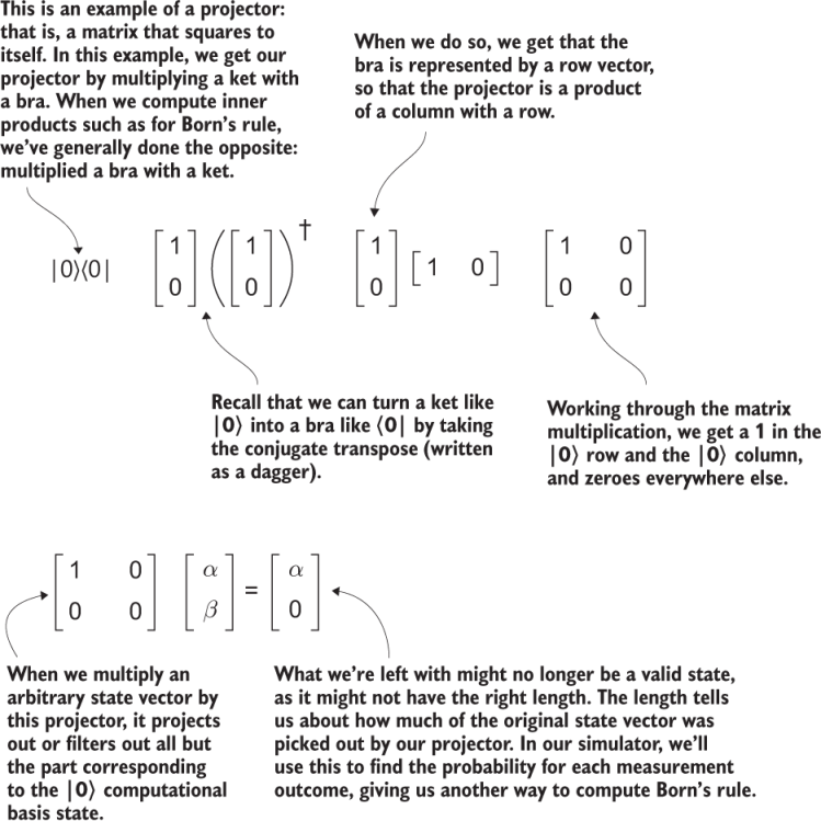
Figure 5.4 An example of a projector acting on a single-qubit state

In QuTiP, we write the bra corresponding to a ket by using the .dag() method (short for dagger, a call-back to mathematical notation we see in figure 5.4). Fortunately, even if the math isn’t straightforward, it winds up not being that bad to write in Python, as we can see next.

Listing 5.13 simulator.py: measuring individual qubits in a register

def measure(self) -> bool:
        projectors = [                                                     ❶
            qt.circuit.gate_expand_1toN(                                   ❷
                qt.basis(2, outcome) * qt.basis(2, outcome).dag(),
                self.parent.capacity,
                self.qubit_id
            )
            for outcome in (0, 1)
        ]
        post_measurement_states = [
            projector * self.parent.register_state                         ❸
            for projector in projectors
        ]
        probabilities = [                                                  ❹
            post_measurement_state.norm() ** 2
            for post_measurement_state in post_measurement_states
        ]
        sample = np.random.choice([0, 1], p=probabilities)                 ❺
        self.parent.register_state = post_measurement_states[sample].unit()❻
        return bool(sample)
 
    def reset(self) -> None:                                               ❼
        if self.measure(): self.x()

❶ Uses QuTiP to make a list of projectors, one for each possible measurement outcome

❷ As in listing 5.9, uses the gate_expand_1toN function to expand each single-qubit projector into a projector that acts on the whole register

❸ Uses each projector to pick out the parts of a state that are consistent with each measurement outcome

❹ The length of what each projector picks (written as the .norm() method in QuTiP) tells us about the probability of each measurement outcome.

❺ Once we have the probabilities for each outcome, we can pick an outcome using NumPy.

❻ Uses the .unit() method built-in to QuTiP to ensure that the measurement probabilities still sum up to 1

❼ If the result of a measurement is |1〉, then flipping with an x instruction resets back to |0〉.

5.2 CHSH: Quantum strategy

Now that we have expanded our simulator to handle multiple qubits, let’s see how we can simulate a quantum-based strategy for our players that will result in a win probability higher than could be possible with any classical strategy! See figure 5.5 for a reminder of how the CHSH game is played.

Figure 5.5 The CHSH game, a nonlocal game with two players and a referee. The referee gives each player a question in the form of a bit value, and then each player has to figure out how to respond to the referee. The players win if the Boolean XOR of their responses is the same as the classical AND of the referee’s questions.

You and Eve now have quantum resources, so let’s start with the simplest option: You each have one qubit allocated from the same device. We’ll use our simulator to implement this strategy, so this isn’t really a test of quantum mechanics as much as that our simulator agrees with quantum mechanics.

Note We can’t simulate the players being truly nonlocal, as the simulator parts need to communicate to emulate quantum mechanics. Faithfully simulating quantum games and quantum networking protocols in this manner exposes a lot of interesting classical networking topology questions that are well beyond the scope of this book. If you’re interested in simulators intended more for use in quantum networking than quantum computing, we recommend looking at the SimulaQron project (www.simulaqron.org) for more information.

Let’s see how often we and Eve can win if we each start with a single qubit, and if those qubits start in the (|00〉 + |11〉) / √2 state that we’ve seen a few times so far in this chapter. Don’t worry about how to prepare this state; we’ll learn how to do that in chapter 6. For now, let’s just see what we can do with qubits in that state once we have them.

Using these qubits, we can form a new quantum strategy for the CHSH game we saw at the start of the chapter. The trick is that we and Eve can each apply operations to each of our qubits once we get our respective messages from the referee.

As it turns out, ry is a very useful operation for this strategy. It lets us and Eve trade off slightly between how often we win when the referee asks us to output the same answers (the 00, 01, and 10 cases) to do slightly better when we need to output different answers (the 11 case), as shown in figure 5.6.

Figure 5.6 Rotating qubits to win at CHSH. If we get a 0 from the referee, we should rotate our qubit by 45°; and if we get a 1, we should rotate our qubit by 135°.

We can see from this strategy that both we and Eve have a pretty easy, straightforward rule for what to do with our respective qubits before we measure them. If we get a 0 from the referee, we should rotate our qubit by 45°; and if we get a 1, we should rotate our qubit by 135°. If you like a table approach to this strategy, table 5.1 shows a summary.

Table 5.1 Rotations we and Eve will do to our qubits as a function of the input bit we receive from the referee. Note that they are all ry rotations, just by different angles (converted to radians for ry).

Input from referee	Our rotation	Eve’s rotation
0	ry(90 * np.pi / 180)	ry(45 * np.pi / 180)
1	ry(0)	ry(135 * np.pi / 180)

Don’t worry if these angles look random. We can check to see that they work using our new simulator! The next listing uses the new features we added to the simulator to write out a quantum strategy.

Listing 5.14 chsh.py: a quantum CHSH strategy, using two qubits

import qutip as qt
def quantum_strategy(initial_state: qt.Qobj) -> Strategy:
    shared_system = Simulator(capacity=2)                   ❶
    shared_system.register_state = initial_state
    your_qubit = shared_system.allocate_qubit()             ❷
    eve_qubit = shared_system.allocate_qubit()
 
    shared_system.register_state = qt.bell_state()          ❸
    your_angles = [90 * np.pi / 180, 0]                     ❹
    eve_angles = [45 * np.pi / 180, 135 * np.pi / 180]
 
    def you(your_input: int) -> int:
        your_qubit.ry(your_angles[your_input])              ❺
        return your_qubit.measure()                         ❻
 
    def eve(eve_input: int) -> int:                         ❼
        eve_qubit.ry(eve_angles[eve_input])
        return eve_qubit.measure()
 
    return you, eve                                         ❽

❶ To start the quantum strategy, we need to create a QuantumDevice instance where we will simulate our qubits.

❷ Labels can be assigned to each qubit as we allocate them to the shared_system.

❸ We cheat a little to set the state of our qubits to the entangled state (|00〉 + |11〉) / √2. We will see in chapter 6 how to prepare this state from scratch and why the function to prepare this state is called bell_state.

❹ Angles for the rotations we and Eve need to do based on our input from the referee

❺ Strategy for playing the CHSH game starts with us rotating our qubit based on the input classical bit from the referee.

❻ The classical bit value our strategy returns is the bit value we get when we measure our qubit.

❼ Eve’s strategy is similar to ours; she just uses different angles for her initial rotation.

❽ Just like our classical strategy, quantum_strategy returns a tuple of functions that represent our and Eve’s individual actions.

Now that we have implemented a Python version of quantum_strategy, let’s see how often we can win by using our CHSH game est_win_probability function.

Listing 5.15 Running CHSH with our new quantum_strategy

>>> est_win_probability(quantum_strategy)    ❶
0.832

❶ You may get slightly more or less than 85% when you try this, because the win probability is estimated under the hood using a binomial distribution. For this example, we’d expect error bars of about 1.5%.

The estimated win probability of 83.2% in listing 5.15 is higher than what we can get with any classical strategy. This means that we and Eve can start winning the CHSH game more frequently than any other classical players—awesome! What this strategy shows, though, is an example of how states like (|00〉 + |11〉) / √2 are important resources provided by quantum mechanics.

Note States like (|00〉 + |11〉) / √2 are called entangled because they can’t be written as the tensor product of single-qubit states. We’ll see many more examples of entanglement as we go along, but entanglement is one of the most amazing and fun things that we get to use in writing quantum programs.

As we saw in this example, entanglement allows us to create correlations in our data that can be used to our advantage when we want to get useful information out of our quantum systems.

Far from being strange or weird, entanglement is a direct result of what we’ve already learned about quantum computing: it is a direct consequence of quantum mechanics being linear. If we can prepare a two-qubit register in the |00〉 state and the |11〉 state, then we can also prepare a state in a linear combination of the two, such as (|00〉 + |11〉) / √2.

Since entanglement is a direct result of the linearity of quantum mechanics, the CHSH game also gives us a great way to check that quantum mechanics is really correct (or to the best our data can show). Let’s go back to the win probability in listing 5.15. If we do an experiment, and we see something like an 83.2% win probability, that tells us our experiment couldn’t have been purely classical since we know a classical strategy can at most win 75% of the time. This experiment has been done many times throughout history and is part of how we know that our universe isn’t just classical—we need quantum mechanics to describe it.

Note In 2015, one experiment had the two players in the CHSH game separated by more than a kilometer!

The simulator that we wrote in this chapter gives us everything we need to see how those kinds of experiments work. Now we can plow ahead to use quantum mechanics and qubits to do awesome stuff, armed with the knowledge that quantum mechanics really is how our universe works.

Summary

• We can use the QuTiP package to help us work with tensor products and other computations we need to write a multi-qubit simulator in Python.

• The Qobj class in QuTiP tracks many useful properties of the states and operators we want to simulate.

• We and Eve can use a quantum strategy to play the CHSH game, where we share a pair of entangled qubits before we start playing the game.

• By writing the CHSH game as a quantum program, we can prove that players using entangled pairs of qubits can win more often than players that only use classical computers, which is consistent with our understanding of quantum mechanics.