6. Adding Outbound Transportation to the Model

Up to this point, we’ve looked at models that have focused mostly on service levels and locating facilities as close to demand as possible. However, running a supply chain costs money. And, sooner or later, someone is going to ask you to financially justify the new supply chain design. That is, you are going to have to determine how much money you will save with the changes you are suggesting.

Transportation is often the most important cost in a network design study. A retail or manufacturing company may spend the equivalent of 2% to 3% of their total revenues on transportation alone. For a company with $5 billion in revenues, this could equate to $150 million in spend. You can imagine that reducing these costs can make a significant difference to the firm’s performance.

It is by design that we have selected transportation costs as the first cost category we discuss in this book. A change in the number and location of facilities often impacts transportation costs more than any other cost in the supply chain. Conversely, manufacturing, purchasing, or product handling costs may be fairly constant no matter where your facilities are. Therefore geographical changes to a network may have less impact on these costs.

In practice, as with service-level models, many network design studies consider only transportation costs. And these studies are perfectly valid. It is much more common to include just transportation costs when you are considering warehouse locations only. But it can happen with studies determining manufacturing locations as well.

To keep with our theme of creating building blocks for more complex models, we will analyze a simple model with a set of facilities that ship directly to customers. Often, this is called outbound transportation. That is, we are shipping “outbound” from our facilities. In later chapters, we will expand our analysis to also include the transportation costs to get product into the facility, from a plant to a warehouse, before it moves on to a customer. This leg of transportation is called inbound transportation. These terms can get confusing when you have multiple levels in the supply chain however. For example, you can have inbound shipping from the raw materials plant to the manufacturing plant before the manufacturing plant then ships product out to the warehouse. You may also have cases in which a product ships through several warehouses (central and regional) on its way to a customer. Despite this, we will stick with the industry-accepted terms throughout the book.

With this introduction of transportation costs into our modeling, we will still be answering the question about where to locate a given number of facilities, but our objective will be to minimize cost, not the average distance.

Sometimes the inclusion of transportation costs to a practical center of gravity model will not change the solution at all, which can be attributed to many factors including the high correlation between distance and transportation costs. It is a good modeling practice to be aware of variables that do not affect the solution. We will cover this further in Chapter 12, “The Art of Modeling.” In many cases, the solution will change as you add transportation costs to the model. There are many different reasons for this:

• Minimum costs in transportation—When you ship a full truckload, there is often a minimum charge assessed independent of how far you go. That is, a carrier may charge $1.50 per mile per truckload, with a minimum of $300. Therefore any shipments within 200 miles will cost the same. This cost structure will cause the optimization to be indifferent when assigning customers to warehouses within 200 miles as the cost will be $300 no matter what.

• Regional differences in transportation costs—Transportation rates are not symmetrical due to the imbalance of supply and demand. That is, a carrier may charge $1.25 per mile to move a full truckload of product from Kentucky to Florida but may only charge $1.10 per mile to move a full truckload of product from Florida to Kentucky. These rate differences are mainly attributed to whether the carrier has demand for its services in the region the truckload is being delivered to. If the carrier can easily find other cargo in that region, the cost to ship into there will likely be cheaper than deliveries to regions where cargo is more sparse and unpredictable. By adding these types of transportation costs to the analysis, the optimization may be able to locate facilities in areas with more favorable rates.

• Different customer shipment profiles—In a single network some customers may always order a full truck’s worth of products at a time, while others may only order a half a truck. When calculated on a per-unit basis, the full-truck customers’ transport costs are much cheaper than the transport costs of those who order in half truck quantities. In these cases, the optimization has an incentive to select facility locations closer to the more expensive half-truck quantity customers.

The only significant difference between this model formulation and the previous practical center of gravity formulation is that instead of a distance matrix, we have a cost matrix. The matrix trans_i,j represents the cost to send one unit of demand from facility i to customer j. For a reminder of how to read this model, see Chapter 3, “Locating Facilities Using a Distance-Based Approach.” As a summary, here is what this model is doing.

The objective of this problem is as follows:

• Minimize the total transportation costs from the facilities (plants or warehouses) to the customers.

We also have the same constraints or rules to keep in mind that we previously defined and discussed in terms of the practical center of gravity formulation:

• We have to meet all the demand. This one seems obvious, but we do not want to minimize the costs by not serving the customer.

• We are limiting the number of facilities to P. If we did not limit the number of facilities and transportation costs were proportional to distance, the optimization engine would likely elect to open and utilize every potential warehouse within the model.

We are making the following decisions:

• Do we use the warehouse at location i? We will denote this decision as X_i. If X_i = 1, then we use the facility at location i; if X_i = 0, then we do not use that facility. This is what is called a binary variable. It can take on a value of only 0 or 1.

• Does facility i service customer j? We will denote this decision as Y_i,j. If Y_i,j = 1, then facility i services customer j. If Y_i,j = 0, then facility i does not service customer j.

There are three things you might not have noticed about the transportation costs when you read the description of the objective function. First, the demand is expressed in total (usually annual) and not shipment by shipment. Second, the transportation costs are expressed in terms of a cost per unit. That is, we are multiplying transportation costs by units of demand, not by shipments. And, third, you need to fill a transportation cost for every possible source and destination, not just the source and destination shipments you used in the past.

We will explore each of these, in turn, in the next several sections.

It may seem more natural to simply model every shipment. Although, in theory, we could try to set up a model with every shipment. In practice, this model would become unwieldy and introduces a false sense of accuracy.

It becomes unwieldy, because if we model every shipment, we have to create a model with potentially hundreds of thousands of shipment points instead of several hundred customer points. We may now have 100 or 1000 times the data to analyze and the size of the model will likely bog down our machine and render the model unsolvable.

But, more important, we have created a false sense of accuracy. As in our discussion in Chapter 1, “The Value of Supply Chain Network Design,” adding every shipment certainly feels more precise. However, it is not more accurate. Remember, we are running models for the future—the next year, the next five years, or maybe even the next month. We are fooling ourselves if we think that we know how the shipments are going to break down, shipment by shipment, over the next year, when we have a hard time predicting aggregate demand over the next month. And, if the customers are served by a different warehouse, then the shipment patterns may change as well. Running a model with many shipments rolled into a single demand point will be as accurate as one with individual shipments.

However, having said that, we do not have to blindly roll up every shipment into an aggregate number. We will discuss this in more detail in Chapter 12 and Chapter 13 “Data Aggregation in Network Design.” But, for now, you can think about refining your demand points to categories like the following:

• Total demand to this point arriving in full trucks

• Total demand to this point arriving in trucks that are half full

• Total demand to this point arriving via overnight express

There are techniques for breaking down the total demand into smaller buckets, but keep in mind that your goal is accuracy and not false precision.

Luckily, with a little math, we can easily convert standard transportation rate structures into a simple cost per unit.

First, for perspective, let’s discuss the many different transportation cost structures. These structures are driven by different modes of transportation (air, road, rail) and even by ways transportation companies quote their rates. When converting transportation rate structures to a cost per unit, we must understand the different types of rates and then apply them appropriately within our model. In practice, commercial network design software will convert a standard rate structure to a cost per unit for the model. However, as a modeler, you must have a good understanding of the rate structures to ensure that the costs used by the model accurately represent reality.

For the purposes of the model, we are interested in the cost to go from facility i to customer j. However, many different transportation providers may make multiple stops between picking up product at facility i and delivering it to customer j. For example, if I order something from a large online retailer that is shipped via UPS from the retailer’s warehouse to my house, UPS may route the product through several of their own warehouses and hubs before actually dropping it off at my doorstep. But, for the sake of modeling, the retailer is only concerned about the single rate that UPS charges them for the delivery and not all the internal UPS movements that take place to ensure that delivery. Here are some of the different modes of transportation and how the rates are typically provided:

• Commercial Truckload or Full Truckload (TL or FTL)—In this mode, a firm is hiring an entire truck to drive from one location to another. The firm is charged for the use of the full truck whether the truck is 100% full or 25% full. The firm does not have to worry about where the truck comes from before the delivery or where it goes after. The trucking company arranges that as part of their own operations. These rates are typically structured either as a flat rate from one point to another or as as a cost per mile or kilometer. If the carrier charges a cost per distance, they may sometimes add a fixed charge on top of that and enforce a minimum charge to prevent very low costs for short moves. The rates charged can vary depending on where the shipment starts and ends. So, two shipments with exactly the same distance, but with different starting points, may have different rates. The carrier contract may also include a separate fuel surcharge which allows the trucking company to manage fluctuating fuel prices without having to recreate each firm’s rates each time. Each of these trucks will have a capacity typically measured in total weight, total cube, or total number of pallets. Also, the term Truckload often lumps a lot of truck types together under the same umbrella. When you are building your model, you may want to consider different types distinctly—regular dry van, refrigerated, flatbed, tanker, 48- and 53-foot trailers, as well as other distinctions that affect the rate applied or the amount of product that can fit within each. Transit time for truckload shipments is normally easily predicted and dependable as less touches are required during transit and it’s a straight shot from one location to the other.

• Private/Dedicated—A private fleet is one in which a firm owns its own trucks. These trucks are used to either deliver full loads to the customer or make multiple stops. A dedicated fleet is similar to a private fleet except that it is owned (and maybe operated) by a third party but dedicated to a single client. The rates for private or dedicated are usually a cost per mile with an optional fixed cost (similar to commercial TL transport described above). Because the firm owns the trucks, they do not need to worry about the rate changes based on the direction of the moves as they would with the use of TL transport. But, they do need to worry about having the truck return. Often, with a private fleet, firms can use the trucks to make deliveries to their customers and then also pick up product from their nearby suppliers on their way back to the origin (this is commonly known as a roundtrip or backhaul). Transit times for this mode are similar to Commercial TL except for the fact that there may be a delay in shipments waiting for trucks to return. If a firm has issues with not having enough vehicles available when needed, they will often supplement their Private/Dedicated transport with Commercial TL transport as well.

• Less-than-Truckload (LTL)—The LTL mode refers to a different transportation market. In the TL market, a truck comes to a firm’s dock door, picks up the product, and directly delivers it to the destination. That truck is dedicated to that firm’s load only. Contrary to what might make sense based on the names, if the firm simply does not fill up the entire truck, it is not referred to as an LTL move. It is still a TL move. A firm goes to the LTL market when it has a small load to ship to a destination where it is not economical to hire an entire truck to make the delivery. In this market, the LTL trucking company picks up the firm’s small load on a route with other firms’ pickups and deliveries. This load then rides with other loads through multiple hubs, where it is placed on different trucks with loads having similar geographic destinations, until eventually loads are placed on a truck departing a final hub to make the trip to complete a route of deliveries to customer locations. However, a firm does not need to worry about these intermediate activities completed by the LTL carrier. The LTL trucking company quotes a single price from origin to destination even if they route the product through different hubs each time. In the U.S. and Canada, these rates are usually based on the source, destination, weight of the shipment, and shipment class (a measure to define the density of the product, whether it is hazardous, and other measures that impact the cost for the carrier to move the item). In Europe however, the LTL market is typically quoted by the number of pallets and the distance it must travel from the source. There are break points in the rates based on some form of capacity level (the more product shipped, the lower the cost per unit to deliver it). Also similarly to TL rate structures, minimums and fuel surcharges are often assessed. As a firm ships larger and larger capacities per shipment a break-even point between shipping via LTL and shipping via TL can be calculated. For example, a TL carrier may hold 45,000 pounds of product, and shipping anything under 15,000 pounds turns out to be cheaper when using the LTL transport mode and rates. LTL shipments typically experience longer transit times however. For the economics to work, the LTL firm will have to send your product through a series of hubs where it may need to wait for other shipments going in the same direction as your load before its final delivery takes place. LTL firms make money when they can fill up trucks with many small shipments and therefore time to destination is sometimes sacrificed in lieu of filling up a truck with more loads per route.

• Parcel—The parcel mode is a lot like LTL but with even smaller shipments sizes. Here a firm is typically charged based on the source, destination and package weight. For heavier packages or shipments, this can be quite an expensive transport mode. However, for packages up to about 150 pounds, it can actually be much cheaper than shipping via LTL. This is because LTL firms are not set up to handle small shipments like specialized parcel carriers. With parcel, there are many service options that give you control over the shipping time, However in most cases, the faster the service the higher the corresponding price. If you want it overnight, the parcel services leverage their more expensive air networks to fly your package. If you are willing to wait, the package moves through their more economical ground network.

• Ocean—Ocean transport is similar to truckload transport but a firm’s product moves in containers (as opposed to truck trailers) across the ocean between port cities (opposed to along highways and local roads). Ocean rates are usually quoted as the cost of a single container from one location to another. The costs can be from port to port or from door to door (where the truck or rail transport to the first port and from the last port is included in the rate). The containers can also vary in size (40-foot, 20-foot) or in capability (refrigerated or ambient). Ocean transit time can be quite long because ocean vessels follow fixed schedules making stops at many different ports along the way.

• Rail—Rail transport moves a firm’s product from one railhead (railcar loading/unloading location) to another. Rail rates are typically expressed in terms of the cost of a rail car to get from one point to another. Like ocean transport, these rates can be between two railheads or from door to door. Most frequent rail shippers have rail lines directly to their plant or warehouse locations. From a transit-time perspective, rail shipments take longer than over-the-road moves (TL, LTL) due to the number of switches and connections required along the way. As a result, they are typically advantageous for cross-country moves with products that are not time-sensitive.

• Intermodal—Intermodal transport combines TL and rail transit. An intermodal move involves a firm’s shipment originally being loaded onto a truck trailer and then delivered to a railhead for transfer onto a flatbed rail car for a portion of the journey. The transfer back to a truck at the destination railhead for final delivery may also take place if the final shipment destination does not have access to its own railhead. These rates typically are expressed as door-to-door rates because the shipping firm handles the full move from origin to final destination. This type of transport can be very economical for cross-continent moves. In terms of costs, intermodal typically falls in between rail and TL transport costs—that is, intermodal is cheaper than TL but more expensive compared to rail. From a transit-time perspective, intermodal takes longer than TL but is faster than rail.

• Multistop—The multistop mode is like the truckload moves, but involves several stops. The multistop mode cost falls between TL and LTL above. In this mode, a firm has several shipments to deliver. The shipments are not all large enough to use a full TL for each however. But together they are too big for an LTL shipment as well. In multistop transit a truck picks up a firm’s load at one facility and then makes deliveries to several destinations. Unlike LTL, the truck is dedicated to just this firm’s loads. The rates are usually expressed in terms of a cost per mile or kilometer with a stop-off charge. The stop-off charges may be waived for the first stop and commonly increase with the number of stops being made on a single route. Often, a trucking company will actually put a limit on the number of stops a single truck will make. There also may be restrictions on the “out of route” miles a single truck may travel within a single route. Out of route is a measure of how far the route deviates from a direct route from the source to the final destination. Multistop transit times are obviously longer than TL which make no intermediate stops from origin to destination. However, multistop transit is typically faster than the use of LTL as the firm has more control of the routes being made and the use of hub locations is much less common. We will discuss multistop in more detail later because they do not always allow for a straight forward calculation of the cost to go from one point to another.

As a side note, a frequent question that arises is: Why not just use the cheapest transportation mode? In general, the more you ship at one time, the lower your transportation costs. That is, if you ship the same total amount, the LTL cost will be lower than parcel, the TL lower than LTL, and Rail lower than TL. In fact, there can sometimes be a nice savings from shifting modes. However, when you ship a quantity too small to be economical for a certain mode, your costs will actually skyrocket. For example, if you hire a full truck to ship a single small package, your cost for that single package will turn out to be quite high. In other cases, you have to make a trade-off between transportation costs and inventory. For example, if a retailer receives LTL shipments once a week from its suppliers, shifting to full truck transit means they shift to only receiving one shipment every six weeks. This change decreases the transportation costs, but will increase the inventory. It is beyond the scope of this book, but firms do mode selection studies frequently to understand the best modes and optimize the trade-off between transportation and inventory.

Now that we understand the different modes and their rate structures, we need to convert the costs to a cost per unit. You should also see that converting to a cost per unit in a mathematical program allows us to standardize the input data. Although some rate structures may require an extra step or two, the basic formula for the cost-per-unit is shown as follows:

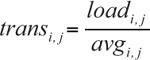
Here trans_i,j is the unit transportation cost we need for our optimization problem, load_i,j is the cost for the load to move from point i to j, and avg_i,j is the average size of the load. As you saw from the above list of modes, most cost structures will directly give you the load_i,j cost. And, if not directly, within a simple step or two.

For some shipment types, determining the avg_i,j is trivial. Assume our units of measure are in pounds. For parcel and LTL, the cost per load is dependent on the size of the shipment. For a ten-pound parcel, the cost of the load will be based on the fact that it is a ten pound shipment and the average shipping size is ten pounds. For an 8,000 pound LTL shipment, the cost of the load is based on an 8,000 pound shipment and the average shipment size is 8,000 pounds.

For TL (and rail, intermodal, ocean, private/dedicated—which are calculated like TL), the average size is the amount that is actually shipped. So, in these modes you are charged to move the whole truck or container or rail car. So you need to figure out how much you actually shipped on the load. For example, you may be given a cost of $800 for a load to go from point A to B. The TL can hold 45,000 pounds. If you ship, on average, 25,000 pounds, that will be the value you use for avg_i,j.

Let’s walk through some examples of how this may be done.

In the example shown in Figure 6.1, we have shown how to calculate the TL load cost based on the shipment distance, the cost per mile, and associated minimum charge. The load cost is based on the larger of the distance rated cost and the minimum charge. For the Chicago to Dallas lane, the distance rated cost ($1.80/mile * 967 miles) was much larger than the minimum charge, while the cost for the Chicago to Indianapolis lane was based on the minimum charge because this was larger than the distance rated cost.

Figure 6.1. Example for Calculating Transportation Cost Per Unit

The determination of the average shipment size (avg_i,j) requires more careful thought however. Of course, we want to determine the average shipping cost over all demand. That is, the cost, trans_i,j, is the cost to go from point i to point j to satisfy all the demand at point j that is satisfied from shipments from point i. It is not just the cost for a single load. So we need an accurate measure of the average shipment size (avg_i,j). For example, in Figure 6.2, we see a sample of lanes and the associated total weight that was shipped along them. By determining the average weight loaded into the vehicles during each shipment, we have an accurate measure of shipment size.

Figure 6.2. Sample Lanes and Average Truckload Shipment Size Data

A commercial network design package will help you with many of these steps. However, it will not do all the thinking for you. You will have to make decisions on the best shipping sizes to use and how to translate your raw data into a working model.

We should keep in mind that we do not want to over-engineer this solution. We want an accurate estimate of the costs, not a precise estimate. The profile of shipment sizes from last year is not likely to exactly match the profile of shipment sizes next year. So close enough is good enough.

• You want the model to evaluate lanes that you are not currently using. As a starting point, you have data on the lanes you are using, but not on the new lanes you want to evaluate.

• Even if your carriers provide you rates, they may only give out “retail” (or non-negotiated) rates until you agree to use that lane and then they will work with you to arrive at a negotiated rate based on the total volume of freight on that lane. The problem is that your existing rates on existing lanes represent negotiated rates. Presumably, if you use new lanes, you would end up with negotiated rates on those lanes as well.

• Your internal data sources are not clean enough to use. The way your data is stored, it is not reliable to determine rates or average shipment sizes.

• You do not have time to gather the data.

In these situations, you may need to estimate the shipping costs. You can do this in various ways:

• Use a simple cost per mile or per kilometer based on the average rates you are paying today. For LTL and parcel, pick a single average shipping size and use the cost estimates tied to that number.

• Use nonnegotiated rates and extrapolate. Often, shipping companies will provide you with a matrix of standard or nonnegotiated transportation rates. Alternatively, there are online services where you can purchase this type of data for specific modes. Then, you can take this information and apply it to all your lanes (current and potential). These rates will most likely be higher than what you are actually paying today. But the trick is to then take the output lane costs for your current lanes and reduce (or increase) them by a uniform percentage so that the total cost on the lanes you use matches the total cost your historical data says you paid. Then apply this blanket percentage reduction (or increase) to all the rates in your purchased data for use within your final model scenarios. This can be an effective way to quickly get accurate rates.

• Use high-level industry benchmarks. We have had success in developing accurate rates using industry-wide average cost per ton-miles published by various independent sources. These rates are commonly expressed as the average cost to move one ton of an item one mile. We have found that generally, in the U.S., the cost per ton-mile in the range of .08 to .11 works well for TL and 0.31 to 0.35 works for LTL. Multistop rate estimates are usually somewhere between the TL and the LTL rates. Parcel rates estimates can be scaled to by three times the LTL rates, and conversely rail tends to only be 50% to 80% of the TL rates. These general rates are good, on average, but have some shortcomings for very short or very long moves.

• Use regression analysis. When you have a lot of shipment data to work with, you can use regression to determine good rates. A simple regression plots the distance of the shipment by its cost. So you can then develop a regression formula to determine a cost based on how far the shipment goes. See the example in the next section.

As an example of using industry benchmarks or published rates in the U.S., you will sometimes find rates provided to and from different states. And sometimes the state designations may be broken down even further. This is because there may be variations in $/mile rates even within a state (from a given origin). This is typically seen in relation to larger states with differences in economic activity across various parts of the state—for example, Northern Illinois (metropolitan Chicago area) has significantly more economic activity than Southern Illinois, thereby yielding a lower $/mile rate. In these cases, it is very common to split a state into subregions—say, California-North and California-South as an example. This provides a better and lower level of granularity. You will need to determine for yourself whether this granularity provides additional significant digits or is just a rounding error however. A sample transportation rate matrix is shown in Figure 6.3 with some states broken into smaller regional groupings.

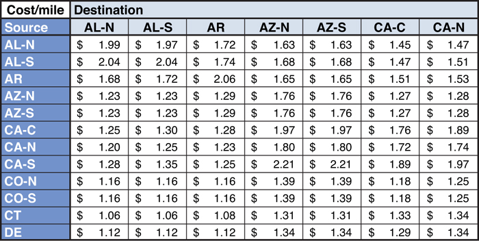
Figure 6.3. Sample Transportation Rate Matrix

Let’s also walk through an example of calculating an average rate for a sample set of data.

In Figure 6.4, we have calculated the cost per mile for each lane in our sample, and an overall average rate as well as a rate by state. To test whether the average is a good measure, we calculate the standard deviation and the coefficient of variation (Std Dev / Average) for both population samples. The standard deviation gives us an absolute measure of variability and the coefficient of variation normalizes the measures and expresses it as a percentage.

Figure 6.4. Cost Per Mile Estimation Based on Average Across Lanes

With this analysis, we see that the overall average rate is $1.79. We would again need to expand our analysis to determine whether we need to worry about the fact that the rate is different to North Carolina versus Ohio.

The shipment table, shown in Figure 6.5, shows the origin location, destination location, shipment weight, and freight cost for each shipment. These are truckload shipments, as can be seen from the shipment weight. As mentioned previously, it is typical for shipments over 15,000 pounds to be delivered using truckload (versus LTL).

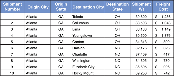
Figure 6.5. Shipment File Sample for Regression Analysis

Our objective is to use this shipment data to derive a $/mile rate that can be used within the model (as we were only given overall shipment costs within the data available).

As a first step, we will calculate the distance for each shipment (or lane). We will then plot the shipments on a chart with freight costs and distance, and perform a regression analysis (using capabilities within Excel).

We will perform the regression analysis (and plot the chart) using the entire sample of ten lanes. This is shown in Figure 6.6. The chart shows that the data fits well along a linear line based on the regression analysis. This shows a calculated rate of $1.83/mile. The regression yields an R² value of 0.95 and statistically significant variables (which you can see if you repeat this example in Excel and explore the output) which validates that this is a good fit.

Figure 6.6. Regression Analysis Based on All Shipments

Here we have simply derived a cost-per-mile rate from the sample shipment data using regression analysis. Of course, in practice, we would want to do a more detailed statistical analysis. This can be accomplished by extending the same type of analysis across multiple origins and destinations to create a rate matrix, showing cost per mile rates on a more detailed state-to-state basis.

However, it becomes more complicated when calculating the costs for the multistop mode. Multistop is commonly used by retailers, but is applicable in other industries as well. With multistop, the final warehouse may send out a truck that makes several stops at different stores on the same route. So the transportation costs are no longer a simple point-to-point rate. The transportation rates will depend on which stores are on which route. And there is no one correct way to allocate the costs of the routes to each individual stop.

If the routes never changed, we would not have a problem because we could just pick a way to allocate the total route costs to each of the stores and we could easily produce accurate costs.

However, the whole point of a network design study is to consider new configurations for the supply chain. This means new warehouses, new assignments, and ultimately new routes.

You might think we would simply change our model formulation to build routes to the customers from the warehouse assignments. We agree that this would be a great approach. However, the limits of mathematics and computation complexity get in our way.

Remember, the number of potential combinations in a network design problem can explode quickly. In Chapter 3, we saw that if we want to pick the best 10 facilities out of 25, we have more than 3 million combinations. If we want to pick the best 10 facilities out of 250, we have 3 million multiplied by 32 billion combinations. It gets even worse very fast if we have to determine the best route out of each of these combinations as well.

Now, let us assume that a warehouse has 50 stores to service and that the routes have five stops each. Using the Excel formula PERMUT gives us the number of total permutations of picking out 5 stores to visit out of the 50 possible. We use PERMUT because any store could be on any route in any order. This yields a total of 254,251,200 possible routes for 5 stores. After that, we still have 45 more stores to cover. If we use the same formula for 45, 40, 35, and so on, we end up with more than 500 million routes to analyze. And this doesn’t include the possibility for routes with 4 stores or 6 stores. If we had 100 stores instead of 50, the number of routes would be more than 34 billion. So a 2-times increase in the number of stores leads to a 68-times increase in the number of possible routes.

If we were to solve both of these problems together, we would effectively need to multiply the number of combinations of warehouse choices by the number of possible routes.

Besides the size issue, there are also differing levels of detail in the routing versus network design problems as well. In our network design problem, we are typically concerned with annual demand and long-term decisions. In routing, we are typically looking at a day’s or week’s worth of shipments. And these shipments may change from day to day or week to week. To make sure that the routes are realistic, we need to worry about things like the shipment sizes, time windows for deliveries, driver rest rules and many more operational constraints.

These problems are simply too large and too complex to combine into one model. And, more important, we do not have to combine them in order to solve our network design problems. We can still develop accurate transportation costs, get good answers, and determine insight into our multistop routes by following the basic principles of a robust multistop approach as follows:

• Worst case, the costs of multistop routes are somewhere between the cost of TL moves and those of LTL moves. For example, we previously mentioned that a reasonable estimate of TL rates is between $0.08 to $0.11 per ton mile and LTL between $0.31 and $0.35. So, multistop rates around $0.15 to $0.25 may be accurate for your model.

• If we compare the equivalent costs of the point-to-point rate with the cost of the route, we can simply adjust the costs with a scaling factor and produce a good answer.

• The network optimization problem is typically a much bigger impact decision and can safely be run first to develop a few alternatives. Then, with each of those alternatives, you can run separate and detailed routing studies to essentially break the tie. Occasionally though, these routing studies may lead you to adjust some costs in your network design model and rerun a few scenarios as well.

To illustrate our approach, we will start with a simple example. We will look at a multistop route from a warehouse to three stores. We will plot the points on a grid and assume straight-line travel distance. We will also assume that costs are directly proportional to distance.

In all the examples, the warehouse is at point (0,0). In all the examples, the warehouse is at point (0,0) and the trucks must all start and end here.

In the first example, shown in Figure 6.7, the three stores in order of the deliveries are at (6,6), (5,10), and (3,8). If we calculate the total distance of this route, we have to calculate the distance between (0,0) and (6,6), between (6,6) and (5,10), between (5,10) and (3,8), and between (3,8) and (0,0).

Figure 6.7. Example Route 1

If we use the simple straight-line distance formula to calculate the distance between two points for our example, (x₁,y₁) and (x₂,y₂) the total distance (and our estimate for cost) comes out to be 23.98.

In our network design formulation however, we only consider the distance from the warehouse directly to each of these points separately. So, how do we compare our total actual distance of 23.98 with how our mathematical model would treat this?

In the mathematical model we consider the distance out and back to these same points. That is, we use the same formula to calculate the distance to each customer, multiply that by two for the trip back, and then add the three distances together. This gives a total distance of 56.42. Now, to make a fair comparison of the multistop route to the 56.42, we need to assume that we run that route three times. That is, presumably we run a multistop route because we want more frequent deliveries. So, in this case, each route delivers one-third of the total requirements for each customer. Therefore, if we run the multistop route three times, we are making a fair comparison to the direct full truckload delivery distances of 56.42. Running the route three times gives us a total distance of 71.94 miles. So we could deliver each store their full requirement with a single truckload shipment, and that total distance would be 56.42. Or make three deliveries on multistop routes, for a total distance of 71.94. It makes sense that the route distance is longer for the multistop in this case—we get the benefit of more frequent deliveries at an additional cost.

In this case, if we want to approximate multistop costs using TL rates within the model, we simply multiply the TL rates by 1.28 (71.94/55.42). Then, our costs in the model will accurately reflect that we are running routes.

This factor will change based on the structure of the routes as well. If the stores are all far away from the warehouse, but close to each other, the factor may be much smaller. In the next example, if the stores are at (6,6), (6.1,5.9), and (6,5.8), then the total two-way distance is 50.6, and running the route three times is 51.3. The illustration in Figure 6.8 shows why these two distances are approximately the same. In this case, the factor is 1.01

Figure 6.8. Example Route 2

If the stores are very far apart, as in the analysis shown in Figure 6.9, the factor will be 1.64.

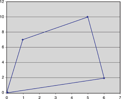
Figure 6.9. Example Route 3

These three examples provide you with intuition on how the factor changes based on the type of routes you run. If the stops are very close to each other and far away from the warehouse, you will have a very small factor. If you run routes with a very long distance between stops, your factor will be closer to 1.5. Experimenting with your data would help determine the appropriate factor. But note that a high factor will be between 1.25 and 1.75.

This section gives you a method for estimating the multistop costs to feed into the model. There may be other methods you can use as well. No method will be 100% accurate, but they will typically be accurate enough for the purposes of your network design work.

The map in Figure 6.10 shows their current supply chain with all shipments shipping out of Louisville, Kentucky. The current cost of this supply chain is $16.6 million. However, as you can imagine, the ground service they currently offer is a bit slow. The average distance to customers is approximately 975 miles. As expected, the breakdown by distance bands (see Figure 6.11) shows a lot of shipments traveling long distances.

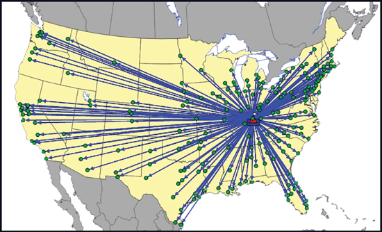
Figure 6.10. Transportation Case Study Baseline Network

Figure 6.11. Transportation Case Study Baseline Distance Bands Summary

This firm wants to determine whether they can reduce costs by opening additional warehouses. They originally assume that adding two additional locations (for a total of three) would be about the right number. Although they are looking to improve their service, they will not make a move unless they can financially justify it first. They first run the optimization to find the best three warehouses.

As you can see in Figure 6.12, when the model is allowed to pick two additional sites, it selects Fresno, California, on the West Coast and Dover, Delaware, on the East. The total cost decreases to $15.2 million, for a savings of $1.4 million or 8% reduction in transportation costs in comparison to their current network. As you would expect, the distance to the customers improves as well. Looking more closely at Figure 6.13, we can see the details of this improvement. The average distance dropped to approximately 430 miles, a more than 50% reduction, and the customers within certain distance bands also improved.

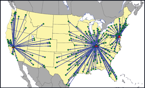
Figure 6.12. Transportation Case Study Best Three Warehouses Solution

Figure 6.13. Transportation Case Study Baseline Distance Bands Comparison

It is not surprising that the distance to customers improved. As mentioned previously in this chapter, transportation costs are strongly correlated with the distance traveled.

Like we’ve seen previously in this book, this firm now wants to understand the marginal value of a fourth warehouse. They determined that if they could get somewhere close to another $1.4 million in savings, it might be worth serious consideration.

When they run the optimization to consider the best four warehouses (results shown in Figure 6.14), the model adds Dallas, Texas, to the previous solution. Note that it did not have to select Fresno, California, and Dover, Delaware but in this case they were still optimal within this solution.

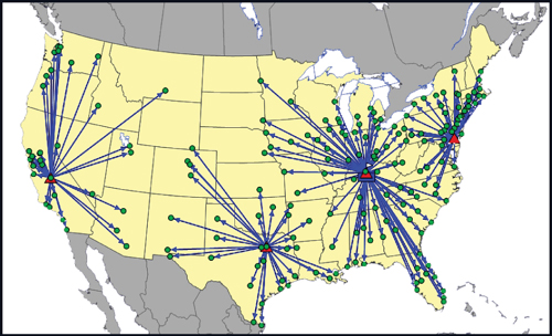
Figure 6.14. Transportation Case Study Best Four Warehouses

In this scenario, the costs decrease to about $15.0 million, which is only a $200,000 savings from their previous 3 warehouse solution (about a 1% reduction). This $200,000 difference also tells us the threshold for the fixed cost. That is, if the fixed cost of the additional facility is less than $200,000, it would still be cost beneficial to open the fourth facility in Dallas. This is a great example of being able to use the information on the fixed cost without having to actually include it in the model. As mentioned previously, we will discuss this concept further within Chapter 12.

In this case, the management team decides that it is worth it to explore adding two warehouses. The $1.4 million was a significant savings, and they could use this to build a strong business case to present to the board. The service improvements will also be a nice part of the business case, but the financial benefits of this are harder to quantify.

However, the management team also felt that they needed to further analyze the costs of the facilities. We will explore these costs in the next chapter.

Transportation costs are often the most important costs in a network design study, and they are the first ones you should consider adding to the model.

These costs come in various forms depending on how product is moved through the supply chain. Although there are some special cases to consider, such as multistop routes and the use of regression to fill in missing rates, transportation costs come down to the fact that you need to apply the appropriate cost per unit to go from Point A to Point B.

It is good to keep in mind the lessons we learned about significant digits when building in transportation rates as well. The details of transportation can get quite complex. But, in the end, you cannot predict the cost of oil or exactly how your customers will order, so your measurements need not be precise enough to discuss costs down to the last dollar either.

When running and analyzing models with costs, keep in mind that the lessons we learned from the models with just distance still apply. It is also good to run multiple scenarios; the additional scenarios can give you the value of an additional facility, and the service metrics still apply.

Finally, we can’t forget that adding the costs does usually help you create a better business case as well.

We will work with the same case mentioned previously in this chapter, except average shipping size per package will change to five pounds. You can find this case and further instructions on the book Web site. The file is called UPS Model 5 lb Avg.zip. Open the model and change the average shipping size to five pounds.

a. Run the baseline model with just the Louisville warehouse and keep the current demand. What is the cost of the baseline?

b. Run additional scenarios for the best two, three, and four warehouses. Which warehouses did it pick, and what is the cost difference between the scenarios?

2. TL and LTL Model—Mini Case Study

A distributor of all types of residential construction products (wood, nails, fixtures, appliances, windows, and so on) delivers product directly to the job site. For small jobs, like a single house, they ship in LTL quantities. For large jobs, like an apartment complex, they ship in TL quantities. They sell to customers across the U.S. and use an average TL rate of $0.11 per ton-mile (with a minimum charge of $12.50 per ton) and $0.30 per ton-mile for LTL (with a minimum charge of $4.00 per ton). The model, more details on the case, and directions on how to use it can be found in the file TL and LTL Model for Construction Products.zip on the book Web site.

a. In the existing supply chain, they are shipping everything from warehouses in Seattle, Dallas, and Pittsburgh. What is the current cost of this supply chain?

b. If they could pick any warehouses from the list of potential warehouses, what are the best three and what is the cost of the best three? What is the average distance to customers, what is the percentage within 300 miles, and how did the average distance to customer change?

c. If they were to add two more warehouses to the existing three, where should they put the warehouses? What is the cost of this solution? What is the average distance to customers, what is the percentage within 300 miles, and how did the average distance to customer change?

d. If they were to pick the best five warehouses, where should they put the warehouses? What is the cost of this solution? What is the average distance to customers, what is the percentage within 300 miles, and how did the average distance to customer change?

3. Transportation Costs and Oil Price—Mini Case Study

The fluctuating price of oil has a big impact on the cost of a supply chain. As oil prices increase, so does the cost of transportation. Recent fluctuations in the price of oil have taught supply chain managers that they need to develop a robust supply chain strategy that performs well if the price of oil is high or low. Also, supply chain managers need to be able to project the amount they will spend on transportation as the price of oil changes. This is a question that gets the attention of the senior management within any firm.

For businesses that ship mostly by truck, we can start to answer this question by understanding how the price of oil impacts the price of diesel fuel. (After we know this, we can approximate how much of our costs are driven by the price of diesel. For other modes of transportation, we can follow a similar methodology.)

Figure 6.15 shows a scatter plot of the price of diesel versus oil. This data can be found on the book Web site in the file Oil and Diesel Prices.xls. This represents weekly data from December 30, 2005, to March 30, 2012.

Figure 6.15. Diesel Versus Oil Cost Regression Analysis

A regression analysis can help us determine the relationship.

a. Run a regression in Excel on this data with the price of diesel as the dependent variable. What is the regression equation that relates the price of diesel to the price of oil? What is the R-squared value? What is the p-value for the independent variable, the price of oil?

b. How much does this model predict that diesel will increase for every $10 increase in the price of oil?

c. Build a chart that shows the expected price of diesel for every $10 increment in the price of oil from $20 a barrel to $200 a barrel.

d. If oil is currently $100 a barrel and you expect it to increase by 40% to $140, what percent increase would you expect in the price of diesel fuel?

e. If oil is currently $40 a barrel and you expect it to increase by 100% to $80, what percent increase would you expect in the price of diesel fuel?

f. How would you use this information when running different network modeling scenarios?

4. Consider a problem in which you need to be able to deliver emergency pharmaceutical products to the drugstores in Chicago. That is, if a drugstore runs out of an item and they need to fill an order, your service can immediately drive the product to their location. You want to determine where your facility should be located to service these drugstores. You also want to minimize the total transportation cost of providing this service. If your transportation provider has come back and told you that the cost to make a delivery is $40, why will this not help you determine the best location for your facility? If the $40 per delivery is all you have, what other objective might you consider to locate your facility?

5. Consider a consumer packaged goods company that sells their products to supermarkets. For the bigger supermarket retailers, they ship full truckloads from their warehouses directly to the retailer’s warehouses. For smaller ones, they will ship their product in full truckloads from their warehouse to local wholesalers who then ship to the stores. This firm is interested in the best locations for their warehouses to minimize the transportation cost. If they have built a cost matrix that has the cost per truckload from every potential warehouse to every one of their ship-to locations, why don’t they need to worry about the distance between the potential warehouses and the ship-to points?

6. When we build a model using expected demand for the next three years, we clearly realize that the demand will be a forecast. Why should you also consider the transportation cost a forecast? What does this tell you about the number of significant digits of accuracy you need for transportation costs in your model?

7. If the cost of an ocean container from China to Seattle is $3,500 and you can fit 250 units into the container, but on average you put in 200, what is the cost per unit that should be used within a network design model?

8. Go to the spreadsheet Raw Transportation Rates.xls on the book Web site. This file shows 300 raw shipments from the warehouse in Atlanta to customers located in Chicago. It shows a mix of TL, LTL, and parcel shipments. Determine the average cost per pound for shipping to Atlanta for each of these modes.

9. If you are working for a firm that ships with multistop truckloads, why might a cost of $0.22 per ton-mile be a good estimate? Assuming that it is a good estimate, why would you want to pick a slightly higher number, or a slightly lower number?

10. In the formulation of this optimization problem, we put in a constraint that limits the number of warehouses to P. If we did not have this in the model, why, in general, would the optimization choose to open and use every potential warehouse? Why is it likely to be a bad decision to open and use every potential warehouse (even though this minimizes the transportation costs to the customers)?

11. In the formulation of the optimization problem, we are assuming that a customer receives many shipments per year. Assume that we are working on a model for a company that makes 25,000 shipments per year. If we model each shipment as a customer point in the model, would this make the model more accurate? (Hint: think about the ability to forecast future demand at this level.) Would this make the model easier to work with and easier to analyze?

12. A manufacturer and distributor of flooring products including carpet, tiles, and hardwood uses a third party with a dedicated fleet to deliver to its customers. The products are picked up from a local warehouse and deliveries are made to customers located within a specific region around the warehouse.

The negotiated transportation rates are based on the following structure:

The truck typically makes multiple deliveries on a trip, so the cost per mile is applied on the total miles driven.

Does this rate structure make sense? Why does the rate increase with an increase in distance? For a customer located 350 miles from the warehouse, what is the transportation cost per unit (assume that there were 300 units per shipment for this customer and that this is the only customer delivered on this trip).

If this company were to optimize the warehouse network using this rate structure in place, how would this impact the locations selected? Would the results be different if there was no minimum charge in the rate structure?