
3. Locating Facilities Using a Distance-Based Approach
As you saw from the examples in the introduction, supply chain network modeling can handle very sophisticated problems. To be able to model, optimize, and develop good solutions to complex supply chains, you need to understand the basics.
In this chapter, we will build on the problem structure developed in Chapter 2, “Intuition Building with Center of Gravity Models,” for Logistica. We will adapt and expand on what we learned by now applying it to a more realistically sized example from the retail industry. We will start with the most basic supply chain network model: optimally selecting “P” facility location(s) considering only distance. This will be your building block for further analysis throughout the rest of the book. You will find that this first step is quite valuable, and some real-world projects may not require more detail.
Retail Case Study: Al’s Athletics
Let’s now begin our analysis of a major retailer in the United States specializing in sporting equipment and apparel named Al’s Athletics. In the late 1960s, Al Alford, a young football coach in a small Texas town many miles away from a major city, decided that the kids in his town shouldn’t be held back because they didn’t have access to the right sporting equipment to practice with. Al felt every kid in his town deserved a chance to become the next great Texas-born sports star. And opening a store close to them to supply the right equipment could be the first step for these kids to grow up to be the next Nolan Ryan, Mean Joe Green, or Olympic gymnast Kim Zmeskal. Before Al knew it, his business was booming. He began selling to parents not only for their children but also for themselves. Al and his family quickly realized that they could repeat their success within similar cities across the south, and 50 years later Al’s Athletics has grown to be one of the largest retail sporting-goods chains in the U.S. Al’s Athletics now has major retail-store outlets in 41 U.S. states.
Al’s grandson (Al the third) is now the CEO and lives and works near the original store in Brownfield, Texas. The family began using a warehouse in nearby Lubbock, Texas, about ten years ago, and the Brownfield Store and many others in Texas have realized great savings in transportation costs and provided significantly better service ever since. Al (the third) realizes that competition in the sporting-goods industry is high, and he has always believed in the philosophy of his grandfather that “proximity to the customer means everything in this business.” As a result, Al wants to look at adding and optimizing warehouse locations across the country to lower costs and provide the best service of any sporting goods chain in the U.S.
In Chapter 2 we used the practical center of gravity analysis to determine a best location for Logistica’s capital city. In this chapter we will build on this idea by now selecting optimal “P” warehouses from a predetermined list of options.
In practice, as mentioned in Chapter 2, most supply chain network design modeling will begin with a set of “potential” facility locations from which to determine the optimal. Let’s begin helping Al by reviewing the formal problem definition for this approach.
Formal Problem Definition for Locating “P” Facilities
Given a set of customer locations and their demand, find the best P number of facilities (plants or warehouses) that minimize the total weighted distance from the facility to the customer, assuming that each facility can satisfy the full demand of the customer and that all demand is always satisfied.
Let’s begin our understanding of this definition by starting with the customers, their location, and their demand.
When modeling a supply chain, the customer refers to the final delivery location for our products. We are only concerned with the final delivery point that is relevant for the supply chain we are analyzing. The product may travel farther before being consumed, but if it is beyond the scope and control of the supply chain we are analyzing, we are not concerned with it.
Depending on the type of supply chain we are modeling, the customer can refer to many types of locations. Each situation is different, and you may need to use various definitions of customers in your supply chain model. Here is just a sample of what a customer location may represent:
• If we are modeling a retail supply chain, the customers may be each of the store’s locations. (The supply chain of Al’s Athletics follows this logic.)
• If the retailer sells directly to their online customers and delivers to the home, the customers may be each ZIP or postal code they ship to. (Later, we will talk about aggregation strategies and the use of postal codes in place of actual home addresses.)
• If the retailer has stores in a shopping mall, they may often ship to the store in a truck that is shared with other retailers in the same mall. To do this, all the retailers ship to a common location, often referred to as a pool point, and then the truck goes from there to the shopping malls for a set fee. In this case, because the assignment of stores to this truck will not change, you may model the pool point as the customer location.
• If we are modeling a manufacturing firm that sells to retailers or wholesalers, the customers could be the warehouses of the retailer or wholesaler. As mentioned previously, from the point of view of the manufacturing firm, they only need to get the product to these warehouses—this is the end of the supply chain for them. The retailers or wholesalers will take it from there.
• If the manufacturing firm ships to other manufacturing firms (say, a steel company shipping to an automaker), the customers will be the other manufacturing sites.
• If a firm’s supply chain already has a fixed and unchanging set of warehouses with a fixed set of customers they service (and this will not be changed), we can model these warehouses as the customer points.
• If a firm’s supply chain services the home-building industry, the customer may represent the job site where we need to provide the product.
• If a company’s supply chain exports product and we are not responsible after the product leaves the country, the customer can be the port of exit.
When we define and discuss customers, we are considering each of the unique ship-to locations as a customer point. For example, a manufacturing company that sells product to a large retailer needs to consider each of the large retailer’s locations they ship to, not a single geographic point representing the retailer, such as the address of the headquarters or a single billing address commonly found within financial data.
“A picture speaks a thousand words” could not be more applicable than to the review of any company’s demand map or customer network. Visualizing customers on a map is a powerful way to start to analyze any supply chain network. In fact, companies can get a lot of value just from this exercise. Let’s start by looking at the customer network for Al’s Athletics.
Figure 3.1 shows Al’s customer points plotted on a map of the U.S. This simple analysis allows you to quickly see where your customers are located, the geographic span of your customer base, and the number of areas you are delivering to.

Figure 3.1. Al’s Athletics Customer Map
We can quickly see that Al’s has stores in most states and a large concentration of stores in Texas (and especially the Dallas area), California, and some points along the East Coast.
To visualize Al’s customers on a map, we needed to link every customer point to latitude and longitude values. This process is called geocoding. Some firms have this data readily available internally. Otherwise, network modeling software can do this for you or there are many Web sites that can provide this data as well.
Now, we need to add demand to the model.
As discussed in Chapter 2, regarding the selection of the capital city of Logistica, optimal location selection often does not make sense based on geography of destination locations alone. The citizens recognized that they wanted to weigh the importance of all city locations by their relative population. Supply chain design studies work very similarly to the way the citizens of Logistica selected their capital; however, these studies use historical or forecasted amounts of product to be delivered to each of the customers as opposed to population. We call this the “demand.” Initially, our models will use demand to determine the relative importance of each customer. For example, a customer who receives 300 truckloads per year of product will be more important than one who receives only 50 truckloads. Of course, in later chapters we will explore the weighting of the importance of customers by other measures as well. But, for now, this assumption will serve us well because it is generally less expensive to be closer to your 300 truckload customer than to be closer to the one with 50.
To specify each customer’s demand, we need to determine the appropriate unit of measure. When thinking in terms of financial systems, we are concerned with the total revenue associated with each customer. However, this unit of measure is not sufficient for network design. In this case, we need a measure that will help us correctly apply the associated manufacturing and logistics costs and capacities. For example, many companies refer to transportation costs in terms of “cost per truckload” and production capacity in terms of “units per hour.” If demand is measured in terms of revenue, we have no way to determine how much “revenue” fits in one truckload or how many dollars of revenue may be produced in one hour. Determining the best unit of measure for demand, production, and transportation is an important step at the beginning of all supply chain models.
For now, let’s assume that we will measure Al’s demand at his stores in terms of total weight (pounds). For example, Store #1 may have a demand of 750,000 pounds of product per year. Al’s selection of weight is probably the most common unit of measure in network design due to the fact that most transportation costs are based on the weight. In later chapters we will discuss modeling demand with multiple products and with different units of measure for transportation, warehousing, and manufacturing cost. Besides weight, other common units of measure include
• Total pallets
• Total cube (physical space the product occupies)
• Total truckloads
• Total cases
This list is just a sample. As you build more complex models, you may find you need to use different units of measure.
The first question Al will face when beginning his demand data collection will most likely be, “What time horizon should we analyze?” Typical network design studies use an entire year’s worth of demand. In addition to being a common reporting time period for many companies, reviewing an entire year of activity within a supply chain ensures that all peaks and valleys of your customers’ buying patterns are accounted for in your analysis.
Imagine a retail company that bases its network design decisions on demand from only a three-month period (January through March). The holiday season has ended and shoppers are hibernating until spring arrives. For some retailers it may be common for their total purchases during this period to be significantly lower than those during the peak holiday months. Designing their network on this data might result in a recommendation to decrease their number of warehouse locations in order to save on capital costs. This company will most likely enjoy their cost savings until the fourth quarter, when a major spike in holiday sales leaves them far short of capacity and facing many problems including lost sales. The cost of this misstep will most likely far outweigh all previous savings. This company will quickly realize that a valuable study needs to incorporate both peak and off-peak periods of demand.
Based on this discussion, Al has provided you with a year’s worth of demand data for the 200 cities in the U.S. where Al’s Athletics stores are located. On the map in Figure 3.2, Al’s customers are sized by their relative demand, and in the second map, we see demand displayed by each state’s relative shading (the deeper the shading, the more demand within that state).
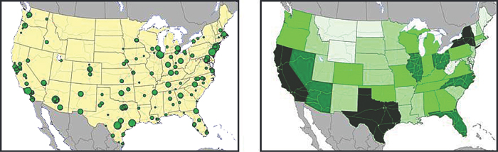
Figure 3.2. Al’s Athletics Customer Maps Formatted by Relative Demand
Returning to our formal problem, if we were asked to write out the current problem that Al is trying to solve, it would be stated as follows:
“Find the best P number of facilities (warehouses) that minimize the total weighted distance from the facility to the customer, assuming that each facility can satisfy the full demand of the customer and that all demand is satisfied.”
With this definition, you can see we are going to assume that our measure of “best” is that we are minimizing the weighted-distance to customers.
We are also going to assume that we are picking our facilities from a predefined set of locations. We will provide Al with a list of the top 25 most frequently selected locations for warehouses in the U.S. to use as a potential list to select from. Adding their current location in Lubbock, Texas, as another potential option, their choices for facilities are shown in Figure 3.3.
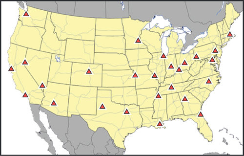
Figure 3.3. Map of All Potential Warehouse Locations for Al’s Athletics
With a predefined set of facilities, we can then build a matrix with the distance between each facility and each customer. In most cases, you are interested in the road distance between two points. This can be easily and automatically calculated with commercial-grade network modeling software.
Formulating and Solving the Problem
We now need a method to solve Al’s problem and others like it.
In Chapter 2, we saw how finding the single-best point was relatively easy. We simply listed all the possible combinations and picked the best one. This would not be too difficult for Al’s problem either, because it would result only in 26 choices.
However, we should not be fooled. The problem gets more complicated very quickly. When we pick the best two sites, we need to figure out the best two locations and determine which customer is served by each of these two sites. Right now, it is easy to assign the customers to the two locations we have chosen—simply pick which of the two is the closest one. However, the complication lies in the number of potential combinations we must consider to prove this. If we have 25 potential facility locations and need to find the best 5, there are 53,130 combinations to evaluate. That is, you would have to evaluate every possible combination of 5 different facilities. The formula for this in Excel is =COMBIN(# of potential facilities, # you want to pick).
Figure 3.4 shows that the number of combinations explodes as you consider more potential facilities. If you add up the total number of combinations for picking between the best two to ten facilities, the total comes to more than seven million options. In this case, there are too many choices to simply enumerate every combination with a spreadsheet.
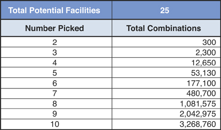
Figure 3.4. Evaluating 25 Potential Facilities Versus Resultant Combinations
The number of combinations can quickly get out of hand if we consider more choices as well. If Al’s Athletics wanted to evaluate 10 times more facilities, the number of combinations they would need to consider for all combinations with two to ten facilities picked would grow by more than 32 billon times the original (see Figure 3.5). In other words, a 10-times increase in the potential facilities leads to a 32-billion-times increase in the number of combinations that need to be considered. It doesn’t take much to find yourself with a potential network design problem containing many more combinations of facilities than the number of atoms in the universe.

Figure 3.5. Evaluating 250 Potential Facilities Versus Resultant Combinations
Based on this information, you can easily see the need for the use of linear and integer programming techniques for sorting through these combinations in a systematic fashion to find the best answer. See the sidebar, “Permutations and Combinations,” for more information.
A casual reader, when confronted with a statement like “There are 53,130 ways to pick the best 5 facility locations from a set of 25 candidates” will tend to take the author at his or her word. There are some diligent readers who will dutifully verify that their Excel spreadsheet displays COMBIN(25, 5) = 53,130 when programmed correctly. Precious few will actually recall the formula that COMBIN applies, and double-check that it is in fact appropriate for this instance.
That’s a shame, because the underlying mathematics here is actually quite intuitive. Understanding the difference between permutations and combinations is useful, in as much as it helps us understand why optimization problems can be so difficult to solve. Moreover, a reader who readily recalls such mathematics has a head start on quickly assessing the difficulty of a wide variety of real-world, combinatorial problems.
To begin with, let’s consider a similar, related problem to the one at hand. Suppose we are trying to select players for a “line” in ice hockey. For those uninitiated into the joys of “Canada’s game,” an ice hockey line consists of three offensemen who skate together. The center, left wing, and right wing all know each other’s styles and habits, and will enter and leave the ice as a trio.
Suppose there are five aspiring players who want to play on the first line. The coach must not only choose which players will skate in the first line, but which positions they will play. Mathematically, this is an example of what’s known as a k-permutation, or a k-permutation of n. The terminology is actually pretty straightforward—k refers to the number of items to select, n refers to the size of the pool from which the selections are made, and the word “permutation” is used because the selections are made into positions.
(A true mathematician would perhaps be more likely to say that one uses permutations when “order matters,” but the difference between “order” and “distinct positions” is a matter of semantics. We were careful to choose hockey as our example because the right wing, the left wing, and the center are considered three distinct positions. When you are selected to skate the right wing, you’d best not skate out to the left side of the rink.)
At any rate, let’s give our five aspiring players useful labels. We will refer to these players as White, Orange, Blonde, Pink, and Blue. Our coach (perhaps himself Mr. Brown) has five choices for who is to play left wing. Suppose he selects Blonde to play this position. The coach now has four choices for who is to play center—one fewer than before, because Blonde cannot play both positions simultaneously. We will assume that the coach selects Blue to center the line. He now has three choices to play right wing (because Blonde and Blue are both occupied). We’ll let this spot go to Orange.
We can write out this selection as (Blonde, Blue, Orange). There are, in fact, 60 such selections for the coach to choose from. The number 60 can be deduced from the number of choices the coach faced at each step: 5 × 4 × 3 = 60.
Although it might seem tedious, let’s write out all 60 choices. We will write them out in a very particular way, in order to serve a purpose that will soon become apparent. For purposes of space, we’ll also shorten their names somewhat.

Again, these are the 60 choices an ice hockey coach has for selecting the first line of his hockey team, when selecting from among a pool of five players.
Now, suppose that rather than selecting the offensive line for hockey, our coach is selecting the three Chasers for a Quidditch team. (If you are reading this book in the year 2050, you might need to be reminded that Quidditch was the game played in the Harry Potter series. This game was later adapted for “Muggle play” by people with lots of creative energy and too much free time—i.e., college students.) The Chasers play a similar offensive role in Quidditch as do the offensemen in ice hockey. However, there is no distinction between the different Chasers. That is to say, a Chaser would not refer to himself as being a “left Chaser” or “right Chaser,” but simply as playing a Chaser.
Thus, when selecting Chasers, the coach would not assign his choices to specific positions. Rather, he would simply name the three players he has chosen. This is an example of an unordered selection, as opposed to selecting hockey players for an offensive line, which is an ordered selection.
Mathematically, the Quidditch-Chaser problem is an example of what’s known as a k-combination, or a k-combination of n. Again, the terminology is straightforward. k refers to the number of items to select, n refers to the size of the pool from which the selections are made, and the word “combination” is used because the selections are made into an interchangeable squad. (Or, more formally, because order doesn’t matter.)
In this case, if the coach were to select the same first-rate athletes as before, then we would write them out as {Blonde, Blue, Orange}. Here, we use {} instead of () because an unordered grouping of players is simply a set, whereas an ordered grouping of players is a “tuple.” (Although the word tuple seems too silly to be real, it is in fact how computer scientists refer to an ordered set. Each one of our 60 offensive lines is a distinct tuple of three players.)
The formula for computing the number of choices there are in a k-combination problem is based on the more straightforward formula we used for the k-permutation problem. Look at the clever way we wrote out our 60 selections above. We arranged them in a grid, with 6 columns and 10 rows. Each row contains the same three players, shuffled into six different combinations. The fact that there are six different combinations per row can be demonstrated from a simpler k-combination problem—if you are restricted to merely selecting the postions for your line from a pool of only three players, then you select from among three choices for left wing, followed by a selection for two choices for center, with right wing being determined by the process of elimination.
Thus, to determine the number of choices for a k-combination of n, we first compute the number of choices there are for a k-permutation of n, and then divide by the number of choices for the k-permutation of k. That is to say, to determine the number of ways to select Chasers from a five-player pool, we first compute the number of ways to select an offensive line from a five-player pool, and then divide by the number of ways to select an offensive line from a three-player pool. The answer in this case is ![]() . It is probably worthwhile to write out these 10 subsets of our five-player pool.
. It is probably worthwhile to write out these 10 subsets of our five-player pool.
{Blnd, Blue, Orng}
{Blnd, Blue, Whte}
{Blnd, Blue, Pink}
{Blnd, Orng, Whte}
{Blnd, Orng, Pink}
{Blnd, Pink, Whte}
{Blue, Orng, Whte}
{Blue, Orng, Pink}
{Blue, Pink, Whte}
{Orng, Pink, Whte}
To formulate these equations in a more general way, we just need to consider the way we counted our coaches’ options for selecting the offensive line. We can note that
where the ! refers to the factorial formula (i.e., 5! = 5 × 4 × 3 × 2 × 1). Thus, the general formula for k permutations of n is ![]()
We can then exploit our observation that k combinations of n is just k permutations of n divided by k permutations of k. Thus, we can derive the Excel formula that started this sidebar:

Note that this last step took advantage of the equation (k-k)!=0!=1. The idea that zero factorial equals one is essentially accepted by definition, and is useful for other aspects of mathematics besides the derviation we demonstrated here.
Finally, knowing the formula for COMBIN (and even better, seeing this formula derived) gives one a gut instinct as to why selection problems can so easily become intractable. At the heart of the COMBIN function lies the factorial function, and the factorial function has a “look and feel” that is very similar to a function that is known for its (sometimes lethal) rapid growth, the exponential function. Indeed a classic mathematical formula, whose proof we will spare you, is based on bounding the factorial formula. Although this formula has multiple names and variations, we will present it as a simplification of Stirling’s formula:
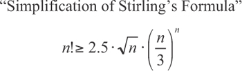
From this formula, we can see that the factorial function is capable of growing very, very quickly, because it will outgrow the complex function to the right, which embeds the exponential function (to see this, test it out in Excel). This is sufficient cause for anyone mathematically savvy to be wary of enumerating the choice selections that are implied by the COMBIN function. That is to say, it is not by accident that we chose to discuss hockey lines and Quidditch Chasers, because more complicated examples would have easily outstripped our ability to type, much less ponder.
Let’s begin by systemically analyzing Al’s Athletics’ problem, based on the criteria we outlined in Chapter 1, “The Value of Supply Chain Network Design.” This will be a generic analysis that can be applied to any similar problem.
Let’s start with the key data elements and define some terminology:
• We have a set of customers we need to serve. We will index this set by the uppercase letter J. So in the case of Al’s Athletics, the set J would be {New York, Chicago, Los Angeles, and so on}. We will call out an individual customer with the lowercase letter j.
• We know the demand of each customer. We will call the demand d and indicate the demand for customer j as dj.
• We have a set of potential facilities we can select from. We will index this set by the uppercase letter I. An individual facility will be designated by the lowercase i. In the case of Al’s Athletics, the facilities are the 25 warehouses.
• We can represent the distance matrix to show the distance from facility i to customer j as disti, j.
The objective of this problem (and Al’s objective) is as follows:
Minimize the average weighted distance from the warehouses to the stores. This is equivalent to minimizing the total weighted distance. However, it is more intuitive to report on the average weighted distance.
We also have a few constraints or rules that we must keep in mind:
1. We have to meet all the demand. This one seems obvious, but we do not want the model to outsmart us by minimizing the distance to a customer by not serving the customer at all.
2. We are limiting the number of facilities to P. For example, Al’s wants to know the best two, three, four, and so on. If we did not limit the number, the model would likely select all facilities. The more facilities, the closer Al’s may be to the customers (our overall objective).
We have two decisions we are making:
1. Do we use the warehouse at location i? We will denote this decision as Xi. If Xi = 1, then we elected to use the facility at location i; if Xi = 0, then we elected to not use this facility. This is what is called a binary variable. It can take on a value of only 0 or 1.
2. Does facility i service customer j? We will denote this decision as Yi,j. If Yi,j = 1, then facility i will service customer j. If Yi,j = 0, then facility i will not service customer j.
We can now formulate this as a mathematical program. Don’t be intimidated by the math here. If this is new to you, this is just a way to systemically describe the problem. You won’t need to understand the mechanics, but instead use the math equations to help build intuition. When we formulate it like this, a standard mixed-integer programming engine can determine the solution. Solving these problems is the subject of many other books and courses and we will not cover the techniques here, although we will provide an example in Excel later in this chapter. However, to understand how these models work, where they become difficult, and how you can implement the results in practice, it is important that you develop good intuition of the underlying concepts.
One way to think about this mathematical formulation is that it gives us a set of rules to make sure we solve the problem correctly. For example, the constraints force us to select the right number of facilities and to meet all the demand. The objective function then guides the search to find a solution that meets our definition of what is best.
The first thing we want to formulate is the objective function. This function gives us the ability to determine whether one solution is better than another. In this case, we want to minimize the total weighted distance from warehouses to customers. So the objective function is to minimize the following equation (1):
The sigma sign (∑) means that we sum whatever comes next (which is why Excel uses this symbol for their calculation button). The letters under the ∑ tell us exactly what we are summing up. The “![]() ” symbol stands for “element of.” In the first summation, we have i
” symbol stands for “element of.” In the first summation, we have i![]() I. So this means that we sum over all the individual facilities in our complete set of potential facilities. The second summation has j
I. So this means that we sum over all the individual facilities in our complete set of potential facilities. The second summation has j![]() J. This tells us to sum over each of the individual customers in our entire customer set. So the entire formula tells us to sum over all facilities and all customers to determine the single answer.
J. This tells us to sum over each of the individual customers in our entire customer set. So the entire formula tells us to sum over all facilities and all customers to determine the single answer.
Note that only Yi,j is a variable. This means that we need to try different values for each of the Yi,j variables. The other terms are input values.
The attentive reader will quickly see why we need constraints. If we simply set every Yi,j to zero (0), the result from the equation will be zero. Zero is certainly a small number However, mathematical optimization techniques are clever and will quickly realize that if we set the Yi,j variables to negative numbers further and further from zero, we will continue to minimize the result of the function. So we see that we need to prevent both of these cases to ensure that the mathematical optimization returns a solution that we can actually use. We will prevent this by now including our constraints.
The first constraint will stipulate that every customer must be fully served. Here, we have an equation for every customer. By using the ![]() symbol, which means “for every,” we can write all these equations simply as (2):
symbol, which means “for every,” we can write all these equations simply as (2):
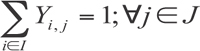
So, starting with the end of the equation, ![]() j
j ![]() J simply means for every customer in the overall set of customers. The first part of the equation states that we sum up all the values of Yi,j for every potential facility and that sum must equal 1. Think of the 1 as representing 100%. So this says that 100% of every customer’s demand must be served. This prevents the problem we mentioned in the objective section where we simply set the Yi,j variables to zero and didn’t serve demand. This now forces the problem to serve all demand.
J simply means for every customer in the overall set of customers. The first part of the equation states that we sum up all the values of Yi,j for every potential facility and that sum must equal 1. Think of the 1 as representing 100%. So this says that 100% of every customer’s demand must be served. This prevents the problem we mentioned in the objective section where we simply set the Yi,j variables to zero and didn’t serve demand. This now forces the problem to serve all demand.
The next constraint stipulates that we want to locate exactly P facilities. The constraint is (3):
The existence of this equation might beg the question: Shouldn’t the optimization engine actually tell us the optimal number of facilities? This is a good question, but for this problem we are interested only in minimizing the average distance to service a customer. So, we have not and do not want to apply a cost of adding a warehouse in the objective function. Because warehouses in this formulation are “free” and we are minimizing just the total weighted distance, there would be nothing preventing the optimization from selecting every warehouse. Is this a flaw in the model? No. We do not want to complicate our model at this stage and the constraint limiting the number of warehouses solves the problem nicely. Besides, our analysis will actually allow us to review a lot of extra information on the value of adding each additional warehouse to our network. This analysis shows that you do not need to directly include every important factor in your mathematical model—through clever analysis, you can often get good information on an important factor without actually modeling it. (You will see this in later chapters as well.)
We still need a way to say that if a warehouse serves a customer in constraint (2), then that warehouse must be considered “open” or “selected.”
For this, we need a way to tie together constraints (2) and (3). If we didn’t have this constraint, the mathematical optimization would simply make good assignments for the Yi,j variables and then randomly pick P warehouses to open. That is, the model may serve the New York stores from the New York warehouse, but decide not to open the New York Warehouse. We display the constraints that make this link as follows (4):
Yi,j ≤ Xi; ![]() i
i ![]() I,
I, ![]() j
j ![]() J
J
Note that we have a constraint for every customer and every facility. If you had 200 customers and 25 warehouses, you would have 5,000 different constraints. (This standard notation allows us to compactly write this as one line.)
We read this constraint (4) as saying that we can’t make an assignment of a warehouse to a customer unless we open that warehouse. That is, if the Xi variable is zero, we cannot assign customers to that particular warehouse.
Now, we need to force the values of X and Y to make sense. In this case we will force these variables to take on a value of either 0 (zero) or 1 (one). For the X variables, this simply means that we either open a warehouse at location i (Xi = 1) or we do not (Xi = 0). It does not make sense to open half of a warehouse. For the Yi,j variables, in this case, we are setting their values to either 0 or 1 as well. In this case, it could, in fact, be logically fine to service a fraction of customer j’s demand from a warehouse. That is, a customer could receive product from multiple warehouses. For now, however, we will set the constraint to require single sourcing of each customer from only one warehouse. Later, we will analyze the impact of this decision and how you can change it. Here are constraints (5) and (6):
When we incorporate all the previously described objectives, decisions, and constraints, here is the mathematical problem formulation of the complete model:
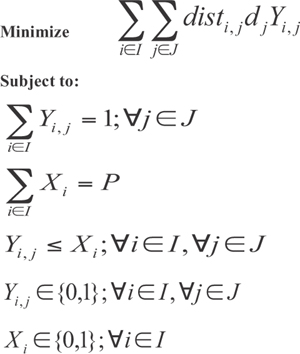
One nice thing about a formulation written like this is that you can solve this for any given set of data. Although we wrote it with Al’s Athletics in mind, it would be equally applicable to other companies. If you solve this with a quality commercially available network design tool, this mathematical formulation will be taken care of for you inside the application. But it is important for you to understand what the network design tool is doing so that you can develop better models and have a clear understanding of the solutions being provided.
It is also important to note what is hard about this problem.
As we saw at the start of this section, there are a lot of different combinations of potential warehouses. There are simply too many combinations to enumerate all the possibilities as we did when we were evaluating the single best location for Logistica. What makes the number of combinations difficult is that there are no reliably efficient techniques for finding the optimal solution when you have binary variables that take on either a zero or a one.
In most cases when you have only discrete variables, the problem falls into a class of problems known as NP-Hard. Without getting into the details and for the purposes of this book, this means that there are no known algorithms that are guaranteed to solve the problems to absolute optimality in a reasonable time as the model size grows. Because this is an engineering and business book, we will take the optimization and computing power as a given and develop ways to build our models so that we get good answers that we can implement.
Certainly, contemporary optimization technology and computing problems allow us to solve very realistically sized problems. We will discuss the size of “reasonable” problems and modeling approaches to ensure that they are solvable throughout the remainder of the book. And based on what we learned previously, we will also keep in mind that the more we avoid adding discrete variables to our model when possible, the better off we’ll be and the larger the models we will be able to solve.
Hands-On Excel Exercise
Another way to think about the formulation of the model is to see it formulated in Excel. The entire formulation with referenced row and column headings can be seen in the Excel file called MIP for 9-City Example.XLS found on the book Web site. The formulation in Excel will not match exactly with our previous algebraic formulation, but it will give us valuable additional insight.
This is a simple model with very few data points so that it can be solved with Excel’s built-in solver. We picked nine cities as customers and used these same nine cities as our potential warehouses.
You can see that the objective function is cell B11, as shown in Figure 3.6. This is the sum of cells B2 to B10. Each cell within B2 to B10 is the sum of demand times the SUMPRODUCT of the appropriate Yi,j column (for Chicago it would be B28 to B36; for Boston it would be J28 to J36) with the matching column in the distance column (for Chicago it would be B41 to B49; for Boston it would be J41 to J49). This is one way we capture the double summation in Excel.
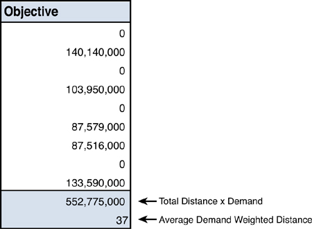
Figure 3.6. Objective Function Portion of MIP for Nine-City Excel Model
The cells C15 to C23 correspond to our Xi decision variables, as shown in Figure 3.7. If we want to place one of the warehouses in the solution, we fill in the corresponding cell value with a 1. We put in a 0 if we do not choose this site.
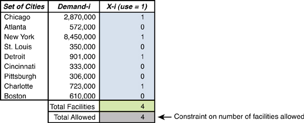
Figure 3.7. Xi Decision Variables Portion of MIP for 9-City Excel Model
The Yi,j variables are B28 to J36, as shown in Figure 3.8. The customers are along the top row and the warehouses are listed in the A column. So if we want the St. Louis customer to be serviced from Chicago, we would fill in a 1 in cell E28. All the other cells in the column for St. Louis should be zero.

Figure 3.8. Yi,j Decision Variables Portion of MIP for 9-City Excel Model
And the distance matrix is shown at the bottom, as depicted in Figure 3.9.
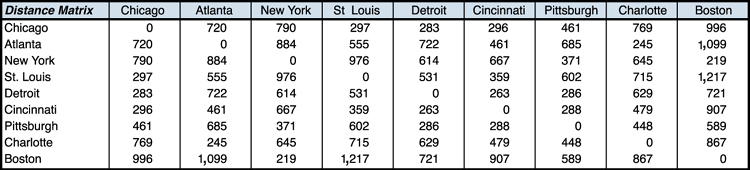
Figure 3.9. Distance Matrix Portion of MIP for 9-City Excel Model
Let’s now take a closer look at the solver (see Figure 3.10). Open the solver dialog box (this requires the use of Microsoft Excel’s “Solver” add-in, see the book Web site for further instructions on how to install and access this functionality), here you will see how we tell Excel’s Solver about the problem. At the top, we fill in B11 and click the “Min” radio button in the “Set Target Cell” and “Equal To” sections. This tells the Solver to minimize cell B11.
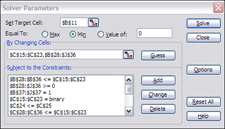
Figure 3.10. Excel Solver for MIP for 9-City Excel Model
The section of the dialog box called “By Changing Cells” is where we tell the solver what our decision variables are. This is what the solver can change.
Next, we fill out our constraints. Unfortunately, the solver does not allow you to order the constraints. So within the list you see that we have constraints that the cells B28 to J36 (the Yi,j decision variables) are set to >= 0. We do not want these to be negative. In this particular problem, these variables will naturally be either a 0 or 1, so we do not have to specify that these will be binary. (Note that this is a special case for this problem and not a general rule.) This is constraint (5).
The cells C15 to C23 (Xi decision variables) are set to binary. So they will be either 0 or 1. This is constraint (6).
We also have a constraint for B37 to J37 to equal 1. This says that each of these cells must be 1. This tells us that we have to meet 100% of the demand. This is constraint (2) from earlier.
We also have a constraint for (3) stipulating that C24 is less than or equal to C25. This tells the model how many facilities it can pick.
As you may recall, constraints (4) within the mathemical formulation are the most complicated and this remains true when creating them in the solver as well. These constraints state that we cannot assign a customer to a warehouse if that warehouse is not open.
To do this in Excel, look at the table that corresponds to the Yi,j variable. Each column represents a customer and each row represents a warehouse. So if we place a “1” in a particular cell, the warehouse corresponding to the row of that cell must be open (otherwise we would have a logical problem of a customer receiving product from a warehouse that was not open). Also note that we’ve created a single column to indicate whether a warehouse is open or closed (this is the Xi table in cells C15:C23). Now, to set the constraint, we just specify that the values in Xi table must be greater than or equal to the values in any single column in our Yi,j table. That is, if we want to put a “1” somewhere in the Yi,j table, we had also better put a “1” in same row of the Xi table. This ensures that we simultaneously make the open and close decisions (in the Xi table) and the assignment decisions (in the Yi,j table). We need to add this constraint once for each column in our Yi,j table—that is, we need to put in this constraint for every customer. These are written as B28:B36 <= C15:C23, C28:C36 <= C15:C23, D28:D36 <= C15:C23, and so on up to J28:J36 <= C15:C23.
This model can now be solved. We will explore this model more in the end-of-chapter questions.
As you will see in the next section, after we solve this problem the resulting solution, when mapped, displays a “star-burst collection” pattern that is characteristic of strategic network design solutions in general (and of center of gravity problems in particular).
Analysis of This Model for Al’s Athletics
Let’s now continue our analysis of this problem for Al’s Athletics.
Our goal is to determine the best P warehouses but we are not assuming that we know the best value for P. Instead, we will run multiple scenarios with different values for P and compare the answers.
In this analysis, we will run the best 1, 2, 3, 4, 5...10 warehouses for Al’s Athletics supply chain. You can see the resultant networks in Figures 3.11 through 3.15.

Figure 3.11. Al’s Athletics’ Best 1 and Best 2 Warehouse Solution Maps
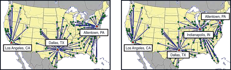
Figure 3.12. Al’s Athletics’ Best 3 and Best 4 Warehouse Solution Maps
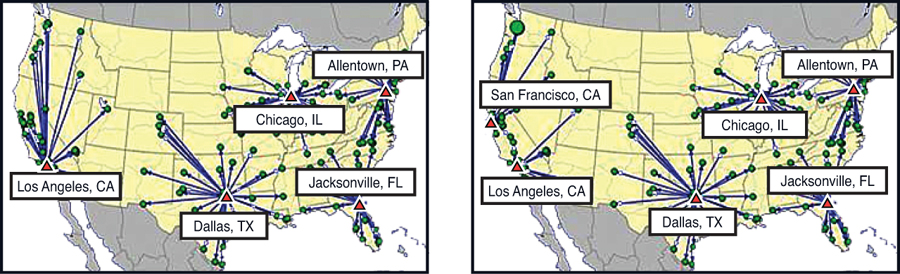
Figure 3.13. Al’s Athletics’ Best 5 and Best 6 Warehouse Solution Maps

Figure 3.14. Al’s Athletics’ Best 7 and Best 8 Warehouse Solution Maps
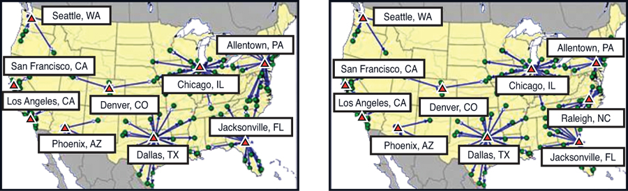
Figure 3.15. Al’s Athletics’ Best 9 and Best 10 Warehouse Solution Maps
We can plot the objective function (in weighted-average distance) for each of the solutions. As you can see from the graph shown in Figure 3.16, there are diminishing returns to adding more facilities. This gives us some insight into the value of an additional warehouse. When we go from three to four facilities, distance decreases by 31%, but when going from four to five, distance decreases by only 19%. We still do not know the best answer, but we now have more insight into value of adding an additional warehouse.
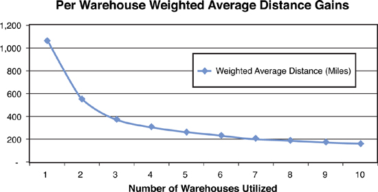
Figure 3.16. Weighted Average Distance Comparison Across Solutions
There is other information we receive from comparing Al’s solutions as well. Weighted average distance is a good summary of service level. However, we can learn more by examining the amount of demand served within certain distance bands or ranges. Figure 3.17 uses bands of 100, 400, 800, and 3,200 miles. In Al’s case, the 100 miles is used to represent demand that is very close to the warehouse, the 400 miles is used for demand reached within a single day, 800 miles for two days drive, and 3,200 miles for all other demand. To read the table in Figure 3.17, look at the 1 Warehouse Solution row. You can see that 1% of the demand is within 100 miles, 4% of the demand is within 100 to 400 miles, 30% of the demand is within 400 to 800 miles, and the remaining 65% is over 800 miles away. In reviewing the full table, we see that solutions improve within each distance band. Demand served within 100 miles, for instance, increases with each new optimal warehouse added to the network. It is important to note that these measures do not necessarily have to improve because they are not part of the objective. But, these distance bands are closely correlated with improving the average distance. That is, by improving the average distance, you are most likely going to have more customers closer to warehouses.
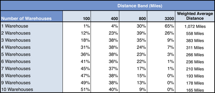
Figure 3.17. Distance Band Comparison Across Solutions
Al now has the information he needs to make a decision. Of course, Al realizes that being closer to his stores and therefore the customers will provide better service and help reduce his transportation costs from the warehouses to the stores (sometimes called “outbound” transportation). He also knows that adding warehouses comes with the cost of extra facilities, extra management time, extra administrative overhead, and extra complexity. (He will have more inventory to manage and suppliers will have to ship to more locations.)
However, Al gets a lot of insight into these costs and complexities with this analysis. He knows that going from one warehouse to two warehouses significantly improves his ability to quickly get product into his stores. And although he might not be able to quantify costs, he knows that going from five locations to six only gets him from 97% to 99% of demand within 800 miles. He may not think this small increase in demand within 800 miles is worth the extra cost of an additional warehouse.
Al still does not have an easy decision. He may still want to do some additional financial analysis on the alternatives before making a final selection. But, for many retailers, having warehouses as close to the stores as possible is the single most important objective. Often, the only question they must answer is exactly how many warehouses and where to locate them.
Lessons Learned from Locating Facilities with a Distance-Based Approach
When you optimize by allowing multiple sites and your objective is to minimize the weighted-average distance, the optimization locates the facilities close to demand. That is, large demand points and areas with a lot of demand will tend to pull locations closer.
This model seems to have a lot of assumptions and a restricted objective function. It is only minimizing the weighted distance. However, do not sell this model short.
First, and most importantly, it is a model that can solve many supply chain network modeling problems. For some firms, ensuring that you are as close to your customers and demand as possible is the most important consideration.
Second, distance is a good measure of your ability to quickly deliver. The closer your facilities are to your customers, the faster you can get product to your customers (assuming your facility has the product ready to ship). So in a supply chain in which response time to customers is important, the model in this chapter may be all that is needed. This is often true for many retailers and similar businesses. Often, the decision making in an organization will require additional financial analysis, but you may be better off doing this outside of your optimization runs.
Third, using these types of models help us realize exactly how much value is gained by each additional facility in your supply chain. These scenarios allowed us to demonstrate to Al that each additional warehouse location offers less benefit to the network on the whole. Knowing exactly how much the benefit diminishes with each additional location allows Al to understand the business implications of adding more warehouses and offering better service to his customers. This helps him “optimize” the Alford family adage of “Service Is Everything.”
Fourth, distance and transportation costs are highly correlated (the farther you have to drive, the more expensive it is). So this model is a good approximation for minimizing the transportation costs to the customers. And, in many cases, this is the most expensive transportation leg.
Finally, although there is a desire for the optimization run to give us a single correct answer, the world is more complicated than that. In practice, when you’re making an important strategic decision, it is more important to run multiple scenarios to understand the trade-offs, and understand the marginal value of adding facilities. This information can then be coupled with strategic business objectives to make a final decision.
Ultimately, this simple model provides a lot of value and can be used as building block for more complicated models.
End-of-Chapter Questions
1. Al’s Athletics has just started the data collection required for you to help them develop their associated network design model. During the first conference call, they indicate that they have three reports they feel could be used to determine the model’s demand per customer. Based on what you have learned in this chapter, which of the following reports could best help us create the demand file? For each of these reports, describe why or why not you could use it to create the demand file.
a. Financial Report listing invoice payments received from all customer accounts over the course of the past year.
b. Warehouse Management System Reports showing inventory levels during each month of the first quarter of last year.
c. Transportation Shipment Report showing origins/destinations, shipment weight, date, and cost over the course of the past year.
2. Al’s data provided us with demand in terms of pounds. Why does this make a good unit of measure for our model? What other units of measure may have been acceptable and why?
3. In the mathematical formulation, what does the X decision variable mean? Why does it have to take on a value of 0 or 1?
4. In the mathematical formulation, why can Y be a continuous linear variable and still give a legitimate solution? (For example, what does a Y value of 0.45 mean?)
5. If you have a problem with 1,000 customers and want to consider 1,000 potential warehouse locations, how many different combinations of choices will you have if you want to pick the best 10 warehouse locations, or the best 25 warehouse locations?
6. Complete the following questions using the MIP for 9-City Example.xls spreadsheet found on the book Web site and reviewed previously in this chapter:
a. What are the best two locations with the given demand?
b. What are the best three locations with the given demand? How much did the average distance decrease?
c. What are the best three locations if you consider the demand for each of the cities to equal 100,000? How does this solution compare to part (b)?
d. What are the best three locations if the demand for every city is equal to 100,000 except New York and Chicago, which are 200,000 each?
7. “Selecting the Best Two to Four Warehouse Locations for Al’s Athletics—Mini Case Study”
This hands-on example will give you your first opportunity to further your understanding of the book’s concepts by building and running scenarios within a commercially available software package. You can get details on the software and data files from the book Web site. The data file you need is called Al's End of Chapter Questions.zip. This file contains additional information to help you with the case study. You will be asked to create and review a slightly altered version of Al’s Athletics supply chain network, as well as prepare and run scenarios in order to determine the network’s best two, three, and four warehouse locations.
a. What are the locations of the best two, three, and four warehouses selected for Al’s network?
b. For each scenario, what are the average throughputs per warehouse? Which warehouse processes the most demand? Which warehouse processes the least?
c. Prepare a quick chart depicting how much demand is serviced within 100-mile, 400-mile, and 800-mile distance bands within each solution. How much more demand can we service within 100 miles utilizing the best four warehouses as opposed to the best two?