
Chapter 16. Scaling MPLS Transport and Seamless MPLS
Today, our industry is experiencing a paradigm shift in service provider (SP) networking: network applications are becoming independent from the transport layers. Modern, cloud-based SP applications need flexible, intelligent overlay network services and are not well-served by legacy, static, low-layer data transmission.
This trend is driven by many factors:
-
Increased demand to bring the service delivery point closer to the user. IP devices are progressively replacing legacy Layer 2 (L2) network elements, hence partitioning the L2 domains.
-
More “intelligent” features for fast protection available at the IP/MPLS layer that could replace the corresponding fast protection features of optical networks.
-
Shifting of mobile traffic—traditionally delivered over TDM circuits—toward Ethernet, and subsequently toward IP in 3G (e.g., Universal Mobile Telecommunications System [UMTS]), or 4G (e.g., Long-Term Evolution [LTE]), or small-cells networks.
-
High-scale data centers shifting to MPLS fabrics and MPLS-enabled servers.
To cope with this demand, increasing the capacity of existing core (or spine) devices is necessary but not sufficient. The required presence of service endpoints in many small-range sites also relies on increasing the overall number of MPLS-enabled devices in the networks.
As a result of bringing the L3 edge closer to the end user, networks are witnessing the introduction of many small devices:
-
In the edge, routers with a relatively small capacity, albeit rich IP/MPLS feature set, some of them targeted as small universal access or cell site access devices.
-
In high-scale data centers, servers and hypervisors with a basic MPLS stack.
The universal edge model provides great flexibility in deploying a service. The edge concept dilutes, and the service termination points can be anywhere in the network. The provider edge (PE) function is distributed in service endpoints, or service termination points. Any device that has a VRF, or that terminates a pseudowire (PW), and so on links the service with the MPLS transport and becomes a service endpoint. In some sense, the function is decoupled from the actual location and type of connectivity of the device.
As for high-scale data centers, implementing MPLS on the servers might end up creating a network with the order of 100,000 MPLS-enabled devices.
Although this MPLS-everywhere approach has many advantages, the introduction of a large number of devices can be challenging. This is especially true if these devices are limited by the amount of state that they can handle and program on their forwarding plane. Segmentation, hierarchy, and state reduction become key properties of the designs and mechanisms that can achieve the required control-plane scalability.
Thus, the Software-Defined Networking (SDN) era networks need to be designed carefully and take into account the control-plane and forwarding-plane scaling capacity of the devices involved.
This chapter discusses several architectural approaches:
-
IP/MPLS scaling with flat LSPs in a single IGP domain (intradomain scaling)
-
IP/MPLS scaling with hierarchical LSPs in a single IGP domain
-
IP/MPLS scaling with hierarchical LSPs in a network split into multiple IGP domains (inter-domain scaling)
-
IP/MPLS scaling with hierarchical LSPs in an IGP-less network
Scaling an IGP Domain
The maximum size of a single IGP domain with MPLS used for transport depends mainly on the control-plane capacity of the weakest router participating in the domain as well as the MPLS transport mechanisms used in the domain. Let’s begin with the IGP.
Note
In this section, the word domain stands for a single OSPF or IS-IS area inside an Autonomous System (AS).
To scale an IGP to potentially the highest possible number of routers in a single IGP domain, you need to follow five major design principles:
-
The IGP should only advertise transport addresses.
-
Preferably only the loopback addresses from the local IGP domain should be injected into the IGP database.
-
In addition, link addresses from the local IGP domain can eventually be injected into the IGP database. In IS-IS backbones where all the core routers speak BGP, it is a common practice to advertise the link addresses via BGP instead of IS-IS. However, OSPF lacks this flexibility, as there is no way to suppress the advertisement of link addresses with OSPF.
-
-
You should avoid redistribution of external prefixes into the IGP.
-
Preferably—apart from the prefixes mentioned previously—no other prefixes should be distributed via the IGP. For example, customer routes should be carried via BGP, which is designed for a much higher scalability than IGPs.
-
In some cases, a limited number of external prefixes (e.g., a default route, routes to a management network, or some summary routes) may be redistributed in the IGP. This situation, however, should be considered as an exception, rather than as rule.
-
-
Prefixes announced via the IGP should be suppressed during flapping. In other words, the prefix should only be advertised if it is stable. This applies to the following prefixes:
-
Prefixes that are inherited from the interface where the IGP is configured. The interface prefix is not advertised until the interface has stabilized (as determined by a fixed hold timer or by an exponential damping algorithm).
-
Prefixes that are eventually redistributed (not recommended, as mentioned previously) from external protocols (e.g., from BGP, or static). The suppression of such prefixes is often questionable and difficult to achieve. Very often, the network administrator responsible of the redistribution point has no authority to influence the configuration (in order to implement some sort of flapping suppression) at the source router where the prefix is originally introduced.
-
-
IGP packets (both Hello packets and packets distributing link state information) should be protected with cryptographic authentication (HMAC-MD5, or newer types of authentication such as different types of HMAC-SHA) to reliably and quickly detect packet corruption and thus improve IGP stability. Standard IS-IS checksum, for example, doesn’t cover LSP ID or Sequence Number fields at all.
-
IGP interfaces should run in Point-to-Point (P2P) mode, whenever possible (the default for Ethernet interfaces is broadcast mode), for more efficient protocol operation and an optimized resource usage at the control-plane level.
With these basic design principles, the number of prefixes carried by the IGP is controlled. All prefixes carried by the IGP are suppressed during flapping; efficient (P2P) operation mode is in place; and IGP packet corruption is detected quickly and reliably. These design principles greatly contribute to IGP scalability and stability during network failures.
Another topic, as outlined in the following sections, is the scaling comparison between OSPF and IS-IS. Although both protocols are link-state, there are some small differences that make IS-IS more stable in very large IGP domains.
Scaling an IGP—OSPF
The Link-State Advertisement (LSA) refresh timer (as specified in RFC 2328, Section B) has a fixed, non-configurable value of 30 minutes (1,800 seconds). Thus, LSAs cause flooding and Shortest-Path First (SPF) calculations relatively often in large networks.
For example, in a stable network with 600 LSAs, every 3 seconds, on average one LSA is reflooded. During network instability, these flooding events are even more frequent.
Junos’ implementation of OSPF uses, by default, 50 minutes (instead of 30 minutes specified in RFC 2328, Section B) of LSARefreshTime for increased network stability. This default can be changed by using the set protocols ospf lsa-refresh-interval command to conform to RFC 2328, if required.
Scaling an IGP—IS-IS
The LSP MaxAge can be approximately 18 times bigger compared to OSPF LSA MaxAge timer (1 hour, according to RFC 2328, Section B.), because in IS-IS this timer is no longer fixed (as described in original specification ISO 10589, Section 7.3.21); it is configurable (RFC 3719, Section 2.1) up to 65,535 seconds (18.2 hours).
RFC 3719, Section 2.1, further specifies that LSPs must be refreshed at least 300 seconds before LSP MaxAge timer expires. In Junos, the LSP refresh timer is not configurable, but is always 317 seconds less than the (configurable) LSP MaxAge timer.
In IOS XR, on the other hand, you can explicitly configure both LSP MaxAge and LSP refresh timer. It is up to the responsibility of the network administrator to configure timers that comply with RFC 3719.
Now, for example, in a network with 600 LSPs, when configuring 65,535 seconds for LSP MaxAge (and 65,218 seconds for LSP refresh) there is on average re-flooding of one LSP every ~109 seconds, which is ~36 times less frequent than in the corresponding OSPF case.
Conversely, the ISO 10589 standard describes the periodic retransmission of Complete Sequence Number PDU (CSNP) packets, which contain the headers (ID, sequence number, lifetime, and checksum) of all the LSPs in the local IS-IS link database. Although the standard only mandates this periodic retransmission over LAN links, Junos additionally performs it over P2P links. This improves the overall network stability thanks to more robust database synchronization, especially when the IS-IS LSP distribution graphs are sparse.
Note
The Junos implementation of IS-IS performs a SPF recalculation at least every 15 minutes for increased reliability.
Warning
Increasing the LSP refresh time increases the amount of time that an undetected link-state database corruption can persist. Thus, it is important to enable cryptographic authentication to minimize the risk of corrupting the link-state database.
Scaling an IGP—MPLS Protocols
Inside an IGP domain, the following techniques are available: Source Packet Routing in Networking (SPRING), Label Distribution Protocol (LDP), Resource Reservation Protocol (RSVP), or a combination of them.
Scaling an IP/MPLS network within a single IGP domain can depend on the MPLS transport method used. With SPRING or LDP, the scaling limits are dictated by IGP itself, rather than by the MPLS transport protocol. So, before reaching any scaling limits related to SPRING or LDP, you would reach IGP limits that would require dividing the single IGP domain into several domains (areas, ASs). Such MPLS scaling architectures based on multiple IGP domains are discussed later in this chapter.
If you use RSVP for MPLS transport (to benefit from a wide range of different protection and traffic engineering features), the network scaling limits may be dictated by RSVP scalability, and not any longer by the IGP. Let’s analyze that in more detail.
Scaling RSVP-TE
The topology illustrated in Figure 16-1 has three layers of routers:
-
Edge (PE) layer: PE1, PE2, PE3, and PE4
-
Aggregation (combined PE/P) layer: P1, P2, P5, and P6
-
Core (P) layer: P3 and P4
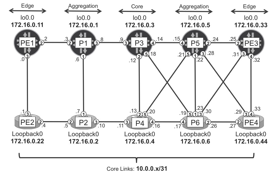
Figure 16-1. Example topology for intra-domain scaling
To provide MPLS-based services (e.g., L3VPN), MPLS transport needs to be established between each pair of routers of the outer (edge or aggregation) layers.
Let’s suppose that RSVP-TE is the only MPLS transport signaling protocol enabled in the network. PE1 signals LSPs toward all of these routers: PE2, P1, P2, P5, P6, PE3, and PE4. This is basically a O(n2) scaling problem, as the number of RSVP LSPs in the network is proportional to the square of the number of endpoints (PE and PE/P layer, in our example). Based on the example topology, the number of RSVP LSPs that need to be established is 8*(8 – 1) = 56. Despite the fact that not all LSPs are traversing all the routers, a proper design needs to take into account possible network failures, which would eventually cause more concentration of LSPs after LSP rerouting. From a scaling perspective, the most affected routers are closer to the center of the core, because they typically concentrate a high number of transit LSPs.
However, RSVP-TE is a unique protocol, and it can do things that no other protocol can do; for example, reserving bandwidth for LSPs. This makes it the core MPLS protocol for big Internet Service Providers (ISPs). Actually, although these core networks typically have very powerful Label Edge Routers (LERs)/Label Switch Routers (LSRs), the actual number of devices is not extremely high. It is high, but it’s nothing compared to universal edge and high-scale data center environments, for which there are many more devices, and these devices have a relatively weaker control plane. That said, ISPs typically prefer not to have a full RSVP mesh due to the O(n2) scaling problem.
There are basically two ways to scale RSVP: on the protocol itself, and with hierarchical designs. RSVP is a stateful protocol, and there are tools to optimize the amount of state and signaling that it can create in large networks with a high number of LSPs.
RSVP-TE Protocol Best Practices
Before discussing hierarchical designs, let’s touch upon basic RSVP features to enhance scaling (and stability) mechanisms, as described in RFC 2961 - RSVP Refresh Overhead Reduction Extensions and RFC 2747 - RSVP Cryptographic Authentication. A well-designed network should use these extensions:
-
Refresh Overhead Reduction Extensions (RFC 2961):
-
Message bundling (aggregation)
-
Reliable message delivery: acknowledgments and retransmissions
-
Summary refresh
-
-
RSVP cryptographic authentication (RFC 2747, RFC 3097)
Without RFC 2961 RSVP generates separate messages for every LSP; as you can imagine, there could be quite a considerable number in very large networks. In addition, the delivery of the RSVP message is not acknowledged by the recipient, which requires a constant refresh of the RSVP state by resending the messages quite frequently.
RFC 2961 addresses this problem in several manners:
- Bundling or aggregating the messages
- Standard Path/Resv RSVP messages are bundled into one large message.
- Introducing the Summary Refresh concept
- Multiple LSP states can be refreshed with a single RSVP message.
- Reliable delivery mechanism
- ACK, NACK, and retransmissions with exponential timers. These mechanisms are similar to the reliable delivery used, for example, in OSPF or IS-IS.
Further steps to increase RSVP’s overall stability can also increase its potential scalability; for example, with the introduction of cryptographic checksums (RFC 2747 and RFC 3097), which improve the reliability in detecting RSVP message corruption.
All these features are supported in both Junos and IOS XR, and example configurations from routers P1 and P2 (Example 16-1 and Example 16-2) are provided for reference. Refresh reduction is enabled by default on IOS XR, whereas you need explicitly enable it on Junos. You need to manually enable cryptographic checksum in both cases.
Example 16-1. RSVP scaling enhancements on P1 (Junos)
groups {
    GR-RSVP {
        protocols {
            rsvp {
                interface <ge-*> {
                    authentication-key "$9$OyXSIhyM87s2alK2aZU.mO1R";
                    aggregate;
                    reliable;
}}}}}
protocols {
    rsvp {
        apply-groups GR-RSVP;
        interface ge-0/0/2.0;
        interface ge-0/0/3.0;
        interface ge-0/0/4.0;
}}
Example 16-2. RSVP scaling enhancements on P2 (IOS XR)
group GR-RSVP
 rsvp
  interface 'GigabitEthernet.*'
   authentication
    key-source key-chain KC-RSVP
 !
end-group
!
key chain KC-RSVP
 key 0
  accept-lifetime 00:00:00 january 01 1993 infinite
  key-string password 002E06080D4B0E14
  send-lifetime 00:00:00 january 01 1993 infinite
  cryptographic-algorithm HMAC-MD5
!
rsvp
 apply-group GR-RSVP
 interface GigabitEthernet0/0/0/1
 interface GigabitEthernet0/0/0/2
 interface GigabitEthernet0/0/0/3
!
Intradomain LSP Hierarchy
Suppose that you need to satisfy the following four requirements at the same time:
-
You need to fully mesh MPLS transport from any PE to any other PE.
-
You want to use RSVP-TE due to its unique feature set.
-
You do not want to face the O(n2) scaling problem associated to establishing the full mesh with RSVP-TE LSPs only.
-
You do not want to split the IGP domain.
In certain network topologies, it is possible to define an innermost core layer within the IGP domain—and without splitting the domain. This layer is typically composed of the most powerful devices in the network and they are a lower number of devices, thereby easing the O(n2) challenge.
For the Internet service, some ISPs run only RSVP-TE on the innermost core layer and they tactically perform IP lookups at the edge of this layer. In other words, the Internet service is only MPLS-aware at the inner core. This can be done with the Internet service because it is an unlabeled one. For labeled services such as L3VPN or L2VPN, it is essential to have end-to-end MPLS on the entire domain.
The solution to this challenge is using LSP hierarchy:
-
The external core devices establish a full mesh of edge LSPs, which may include the internal core devices (as endpoints), too. This edge LSP layer can naturally be built with LDP or SPRING, and with some tricks, also with RSVP-TE (this will be discussed soon).
-
The internal core devices establish a full mesh of core LSPs based on RSVP-TE.
-
The edge LSPs are tunneled inside the core LSPs.
You can view the edge and core LSPs as client and server LSPs, respectively.
Let’s look at the different options available to achieve this kind of LSP hierarchy. These options can coexist. Remember that you can configure several global loopback addresses on the PEs and create different service planes, each with its own MPLS transport technology (for more details, go to Chapter 3). Additionally, you can still signal flat (nonhierarchical) RSVP-LSPs between two edge devices in a tactical manner, because you need it for a given service and not for full-mesh connectivity requirements.
Tunneling RSVP-TE LSPs Inside RSVP-TE LSPs
Pure RSVP-TE LSP hierarchy concepts are described in RFC 4206. Figure 16-2 illustrates the idea with two LSPs:
-
A core P1→P5 LSP with two hops: P1→P3 and P3→P5
-
An edge PE1→PE3 LSP with three hops only: PE1→P1, P1→P5 and P5→PE3
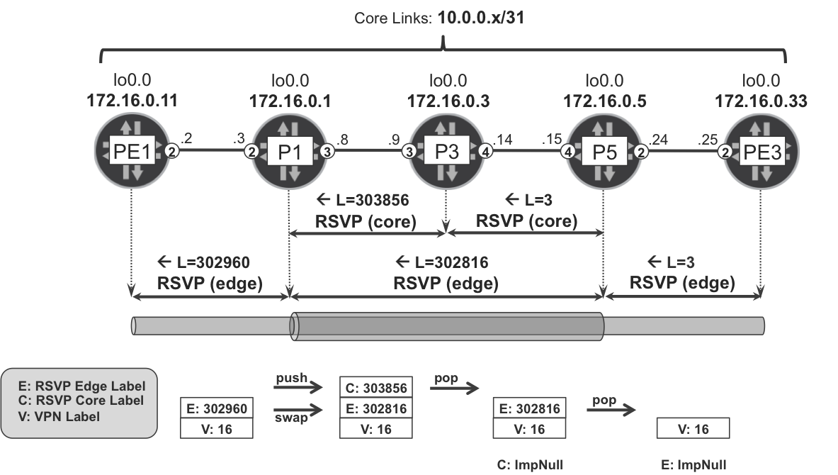
Figure 16-2. Tunneling RSVP-TE LSPs inside RSVP-TE LSPs
Because P1 and P5 are not directly connected, the core LSP is responsible for tunneling the edge LSP, so the P1→P5 path looks like one hop. The inner LSR (P3) is totally unaware of the edge LSP, reducing the state and signaling that P3 needs to handle. As for P1 and P5, they keep some edge LSP state, but only for their geographical region.
As of this writing, this model is not supported in IOS XR, and in Junos it is only implemented for networks using OSPF as the IGP. For this reason, this book does not cover it in detail.
Tunneling LDP LSPs Inside RSVP-TE LSPs
This model, commonly called LDP tunneling, covers a slightly different case. Although this time the network design still requires RSVP-based traffic engineering features in the core, these features are no longer required in the edge.
Based on the sample topology presented in Figure 16-3, Example 16-3 and Example 16-4 contain the basic configuration required to implement LDP tunneling in Junos (P1) and IOS XR (P2) devices. A similar configuration needs to be deployed on P5 and P6 routers, too. LDP tunneling is currently supported for IS-IS and OSPF in both operating systems. This example uses IS-IS and the metrics are left to the default value (10) except on the PE1-PE2 and PE3-PE4 links, where it is set to 100.

Figure 16-3. LDP Tunneling topology
Example 16-3. LDP tunneling configuration at P1 (Junos)
groups {
    GR-LSP {
        protocols {
            mpls {
                label-switched-path <*> {
                    ldp-tunneling;
                }
}}}}
protocols {
    rsvp {
        interface ge-0/0/1.0;
        interface ge-0/0/3.0;
    }
    mpls {
        apply-groups GR-LSP;
        label-switched-path P1--->P2 to 172.16.0.2;
        label-switched-path P1--->P5 to 172.16.0.5;
        label-switched-path P1--->P6 to 172.16.0.6;
        interface ge-0/0/1.0;
        interface ge-0/0/2.0;
        interface ge-0/0/3.0;
    }
    ldp {
        interface ge-0/0/2.0;
        interface lo0.0;
}}
Example 16-4. LDP tunneling configuration at P2 (IOS XR)
interface tunnel-te1
 signalled-name P2--->P1
 destination 172.16.0.1
!
interface tunnel-te5
 signalled-name P2--->P5
 destination 172.16.0.5
!
interface tunnel-te6
 signalled-name P2--->P6
 destination 172.16.0.6
!
rsvp
 interface GigabitEthernet0/0/0/1
 interface GigabitEthernet0/0/0/3
!
mpls traffic-eng
 interface GigabitEthernet0/0/0/1
 interface GigabitEthernet0/0/0/3
!
mpls ldp
 interface tunnel-te1
  address-family ipv4
 !
 interface tunnel-te5
  address-family ipv4
 !
 interface tunnel-te6
  address-family ipv4
 !
 interface GigabitEthernet0/0/0/2
  address-family ipv4
!
The following major configuration elements can be emphasized from this example:
-
RSVP is enabled only on the interfaces toward the core (P routers), and is no longer enabled on interfaces toward the edge (PE routers).
-
LDP is enabled on the interface toward edge (PE routers) as well as over the RSVP tunnels. In Junos, you need to explicitly enable LDP on the loopback interface.
Note
As a best practice, you can also enable LDP on all the IS-IS interfaces, providing a backup MPLS transport mechanism.
When LDP tunneling is enabled, the aggregation routers establish LDP sessions that are targeted to the remote end of the P→P RSVP LSPs, as visible in Example 16-5 and Example 16-6. The word “targeted” here means not necessarily between directly connected neighbors. These sessions make it possible for the routers to exchange the LDP labels required to establish end-to-end forwarding paths.
Example 16-5. Targeted LDP session on P1 (Junos)
juniper@P1> show ldp session
  Address      State        Connection     Hold time  Adv. Mode
172.16.0.11    Operational  Open             26         DU
172.16.0.2     Operational  Open             25         DU
172.16.0.5     Operational  Open             27         DU
172.16.0.6     Operational  Open             22         DU
Example 16-6. Targeted LDP session on P2 (IOS XR)
RP/0/0/CPU0:P2#show mpls ldp neighbor brief
Peer               Up Time     Discovery  Address  IPv4 Label
-----------------  ----------  ---------  -------  ----------
172.16.0.22:0      1d01h               2        4          10
172.16.0.1:0       1d01h               1        2           9
172.16.0.5:0       00:38:41            1        3           8
172.16.0.6:0       00:38:44            1        7          10
The targeted LDP sessions exchange LDP bindings for the access PEs (PE1, PE2, PE3, and PE4). A targeted LDP session, viewed as one piece of the LDP end-to-end LSP, exchanges label bindings to “glue” together other LDP LSP segments. These other segments are signaled with hop-by-hop LDP sessions outside the RSVP domain.
LDP tunneling in action
Let’s suppose that an IP VPN service is provisioned on all the PEs and, according to the BGP next hop, a user packet needs to be label-switched from PE1 to PE4.
The key piece is the following label exchange. P1 learns from P6 the label value 16022 to reach the loopback of PE4 (172.16.0.44).
Example 16-7. FEC binding over targeted LDP on P1 (Junos)
juniper@P1> show ldp database session 172.16.0.6 | match <pattern>

Input label database, 172.16.0.1:0--172.16.0.6:0
  16022      172.16.0.44/32
Output label database, 172.16.0.1:0--172.16.0.6:0
 299808      172.16.0.44/32
As a result of this signaling, P1 installs the entry shown in Example 16-8 in its LFIB.
Example 16-8. LDP tunneling—forwarding plane on P1 (Junos)
1     juniper@P1> show route label 299808 table mpls.0
2
3     299808  *[LDP/9] 00:00:20, metric 30
4              > to 10.0.0.9 via ge-2/0/3.0, label-switched-path P1-->P5
5              > to 10.0.0.9 via ge-2/0/3.0, label-switched-path P1-->P6
6
7     juniper@P1> show route forwarding-table label 299808
8
9     Routing table: default.mpls
10    MPLS:
11    Destination  Type RtRef  Type Index    NhRef
12    299808       user     0  ulst 1048579     2
13    Next hop                                 Index  NhRef Netif
14    10.0.0.9  Swap 300016, Push 300112(top)    556     1  ge-2/0/3.0
15    10.0.0.9  Swap 16022, Push 301104(top)     563     1  ge-2/0/3.0
Due to the classical Equal-Cost Multipath (ECMP)–awareness of LDP, the traffic is load-balanced between the following equal-cost paths:
-
PE1→P1→P3→P5→PE4 (lines 4 and 14).
-
PE1→P1→P3→P6→PE4 (lines 5 and 15).
Figure 16-4 shows the signaling and forwarding-plane details for an L3VPN user packet that flows through the second path: PE1→P1→P3→P6→PE4.
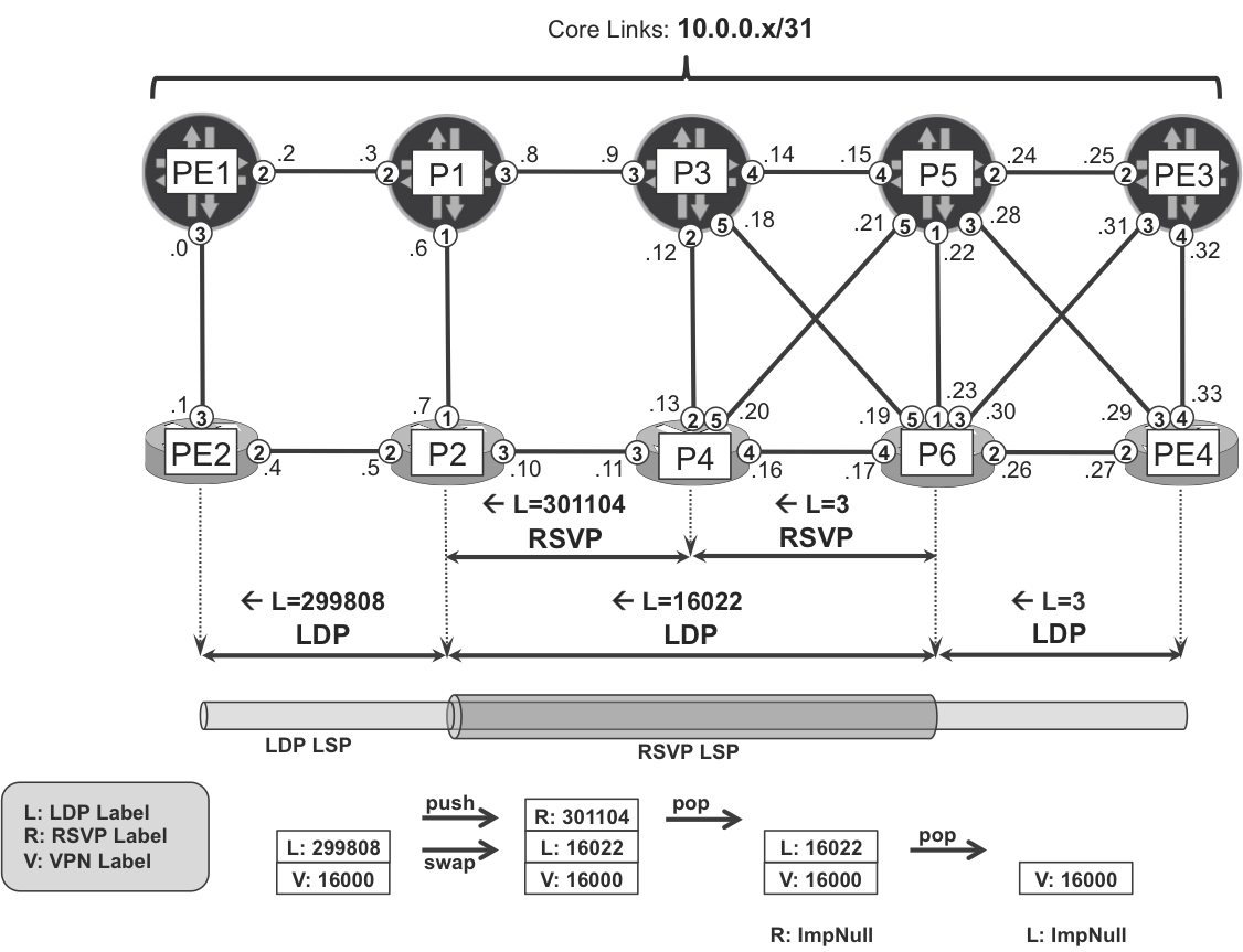
Figure 16-4. Tunneling to-PE4 LDP LSP in P1→P6 RSVP-TE LSP
The label stack in the core now has three labels, from top to bottom: the RSVP label, the LDP label, and the VPN label.
Tunneling SPRING LSPs Inside RSVP-TE LSPs
This model is very similar to LDP tunneling, with one important difference: it does not require any extra signaling. There is no strict equivalent to the targeted LDP session. As you know, IGP-based SPRING encodes segment information in the Link State Packets, and LERs/LSRs automatically translate these segments into MPLS labels. This solution is therefore operationally simpler than LDP tunneling.
Like LDP, SPRING is natively ECMP-aware, so there are several possible paths. This example focuses on the PE1→P1→P3→P6→PE4 path, as shown in Figure 16-5.
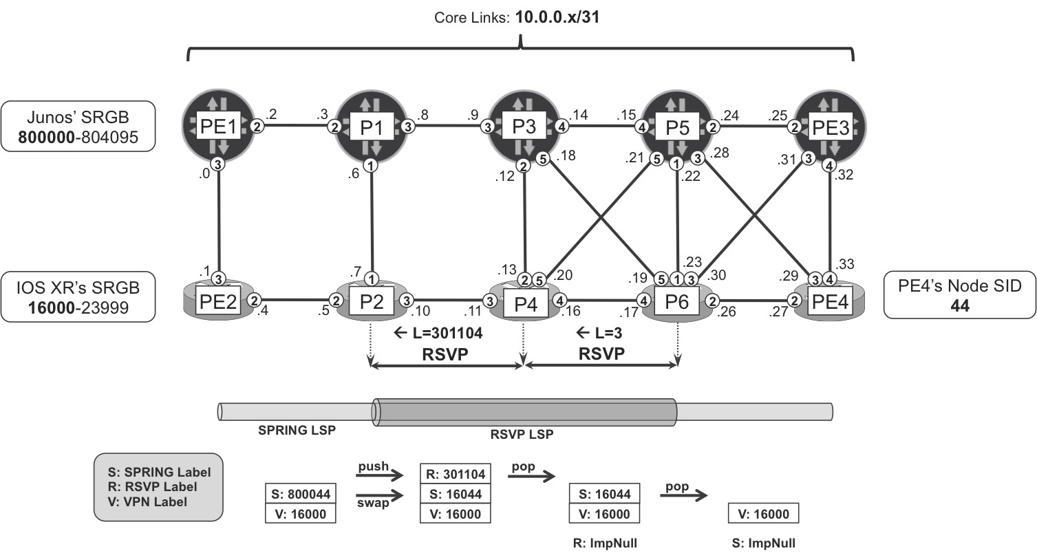
Figure 16-5. Tunneling to-PE4 SPRING LSP in P1→P6 RSVP-TE LSP
This is the path followed by a user packet that is label-switched from PE1 to PE4:
-
PE1 pushes the VPN label and the SPRING label calculated from P1’s Segment Routing Global Block (SRGB) and PE4’s node SID, and then sends the packet to P1.
-
P1 swaps the incoming SPRING label for the SPRING label calculated from P6’s SRGB and PE4’s node SID. Then, it pushes the transport label associated to the RSVP-TE LSP P1→P6 and sends the packet to P3.
-
P3 pops the RSVP label and sends the packet to P6.
-
P6 pops the SPRING label and sends the packet to PE4.
Let’s have a look at the forwarding state at P1.
Example 16-9. SPRING shortcuts on P1 (Junos)
juniper@P1> show route label 800044 table mpls.0

800044  *[L-ISIS/14] 00:00:21, metric 30
         > to 10.0.0.9 via ge-2/0/3.0, label-switched-path P1-->P5
         > to 10.0.0.9 via ge-2/0/3.0, label-switched-path P1-->P6

juniper@P1> show route forwarding-table label 800044

Routing table: default.mpls
MPLS:
Destination  Type RtRef  Type Index    NhRef
800044       user     0  ulst 1048596     2
Next hop                                 Index  NhRef Netif
10.0.0.9  Swap 800044, Push 300112(top)    576     1  ge-2/0/3.0
10.0.0.9  Swap 16044, Push 301104(top)     593     1  ge-2/0/3.0
This tunneling mechanism is enabled in Junos with the following syntax, assuming that the IGP is IS-IS:
Example 16-10. Configuring TE shortcuts on P1 (Junos)
protocols {
    isis {
        traffic-engineering {
            family inet {
                shortcuts;
}}}}
This configuration basically installs the RSVP-TE LSP as a next hop for all the destinations that are at or behind the tail end.
You can achieve the same behavior in IOS XR by using the autoroute announce command.
Interdomain Transport Scaling
As a network grows, it might no longer be possible to keep a single IGP domain. The network is often divided into multiple IGP domains to cope with the increased scale requirements. This is especially important when low-end devices with limited scalability are deployed. Depending on the actual design requirements, the division can be based on different IGP areas, different (sub)ASs, or a combination of the two.
Note
In this chapter, splitting the network in different domains has a scaling purpose. The context is therefore different from that of Chapter 9, where each AS really represented one single administrative domain.
From the MPLS perspective, multidomain transport architectures add additional challenges. To provide end-to-end services (e.g., L3VPN) across multiple domains, you can consider two high-level approaches:
- Nonsegmented tunnels
- End-to-end transport LSPs established across domains and service provisioning only takes place at the LSP endpoints. This model is conceptually aligned to inter-AS Option C, and it typically relies on LSP hierarchy. The next-hop attributes for the service BGP routes are not changed at the boundaries.
- Segmented tunnels
- Transport LSPs span only a local domain and service-aware “stitching” takes place at the domain boundaries (Area Border Router [ABR], Autonomous System Border Router [ASBR]). This model is conceptually aligned to inter-AS Option B, and in it, next-hop attributes for the service BGP routes typically are changed at the domain boundaries.
Both approaches have their advantages and disadvantages. Depending on the scaling capabilities of the devices deployed in the network, functional elements of both architectural solutions can be found in most typical large-scale IP/MPLS designs.
Let’s begin the discussion covering the options to provide nonsegmented, end-to-end transport LSPs across a divided network; we’ll leaving the service stitching concepts for the Chapter 17, which focuses on service scaling. Nonsegmented tunnels can be further classified as Nonhierarchical and Hierarchical. Let’s look at each of them in detail.
Nonhierarchical Interdomain Tunnels
To provide end-to-end transport LSPs across domains, you can use different techniques:
-
Redistribution of /32 loopback addresses between IGP domains, to enable end-to-end LDP-based LSPs between IGP domains. This is in conformance with LDP specification (RFC 5036), which requires an exact match between routing table prefixes and the FECs to which labels are mapped.
-
Redistribution of summary routes (loopback address ranges) between IGP domains. This is in conformance with LDP inter-area (RFC 5283), which relaxes the requirements of RFC 5036 by allowing nonexact matches. It also relaxes the stress on the IP routing tables in very-large-scale networks. Now, FEC label bindings can still be processed if they match a less-specific prefix (e.g., a default route), even if the exact /32 route is not present in the routing table.
-
RSVP inter-area LSP, based on RFC 4105.
Note
Inter-area SPRING has not been explored in this book’s tests.
The real benefit of the LDP-based or SPRING-based interdomain solutions is their simplicity.
The first option (loopback redistribution) can still suffer from IGP/LDP scalability problems, especially on low-end devices. The size of the IGP database, the IP Forwarding Information Base (FIB) and the MPLS FIB might still be too big.
The second option (loopback summary redistribution) relaxes the scaling issue associated with the IGP and IP FIB size, but still might cause MPLS FIB scalability problems. Indeed, LDP bindings for all the loopbacks are still exchanged among IGP domains.
One way to mitigate this problem is to apply LDP policies at the IGP domain boundary, in such a way that redistribution takes place only for selected FECs. Another option is to deploy LDP Downstream on Demand (DoD) in access domains. Unlike the default label distribution method in LDP (downstream unsolicited), DoD makes it possible for low-scale devices to request labels for selected FECs only.
In many cases, the operational challenge lies on the definition of a set of selected FECs. If the low-scale access PEs provide only L2 PWs, the selection is quite obvious: only labels for the remote endpoints of L2 PWs are required. If, however, multipoint services such as L3VPNs are implemented, as well, the definition of selected FECs is no longer straightforward, unless there is a limited number of hub-and-spoke–style L3VPNs only. Another method to mitigate the problem is a service design that removes the requirement to have label bindings for remote loopbacks, which is discussed in detail in the Chapter 17.
Many network operators rely on traffic engineering (TE) techniques, so RSVP becomes their preferred protocol. Although inter-area RSVP is an option, its scalability is limited. There is a conceptual conflict between dividing the network in smaller pieces (domains) while maintaining an end-to-end RSVP LSP full mesh. Therefore, although you can use inter-area end-to-end RSVP LSPs tactically in some scoped scenarios, they are not a generic strategy to fully mesh all the PE routers in large-scale networks.
Hierarchical Interdomain Tunnels (Seamless MPLS)
Let’s discuss the most robust scaling architecture that is available for ISPs.
Seamless MPLS overview
Scaling and BGP often go hand in hand. In this approach, whereas the MPLS transport inside each IGP domain is provided by LDP, RSVP, or SPRING (or by a combination of these), end-to-end LSPs between domains are provided by BGP. The architecture is relatively new, and it is defined in draft-ietf-mpls-seamless-mpls. In reality, this model is based on a mature protocol (BGP labeled unicast: RFC 3107). What’s new is how this protocol is used to provide a very scalable MPLS architecture, supporting up to 100,000 routers.
At a high level, Seamless MPLS is similar to the aforementioned LSP Hierarchy concept. Each IGP domain establishes standard intradomain LSPs by using LDP, RSVP, or SPRING. Tunneled inside these intradomain LSPs, there are other—interdomain—LSPs based on the BGP Labeled Unicast (BGP-LU) protocol. Why choose BGP-LU? Because of its proven scalability.
Chapter 2 explains BGP-LU in the context of flat (nonhierarchical) LSPs. Chapter 9 goes one step further by showing hierarchical LSPs; however, for a slightly different use case: interprovider services. Now, let’s see how to build hierarchical LSPs in a single organization domain, which is partitioned in different areas and/or ASs.
It is important to remember that BGP-LU carries information about provider infrastructure prefixes. The label in BGP-LU is a transport (and not a service) label, mapped to the global loopback address of a PE router. In that sense, you can view BGP-LU as a tool to interconnect different routing domains.
In contrast, a PE router is typically the endpoint of an MPLS service such as L3VPN, L2VPN, and so on. This is the service context of BGP, implemented through other NLRIs such as IP VPN and L2VPN, as already discussed in Chapter 3 through Chapter 8.
Note
If you read Chapter 9, this paradigm might sound familiar to you. Indeed, Seamless MPLS has much in common with Inter-AS Option C.
Let’s use a bigger example topology to discuss the Seamless MPLS architecture, as illustrated in Figure 16-6.
In Figure 16-6, the network is divided in two ASs: 65001 and 65002. Moreover, AS 65002 is further divided in two IS-IS domains: an L2 domain with area ID 49.000, and an L1 domain with area ID 49.0001. There is no IS-IS route exchange between the two domains: both L1 to L2 leaking and L2 to L1 leaking are blocked. The L1 routers are explicitly configured to ignore the attached bit of the ABR’s L1 Link State PDUs. This example uses different MPLS protocols inside the different domains to show that they are completely independent from one another. Thus, there is plain LDP in IS-IS L1 area 49.0001, LDP tunneling–over-RSVP in IS-IS L2 domain, and plain RSVP in OSPF area 0.0.0.0. In some sense, you can look at this architecture from different angles.
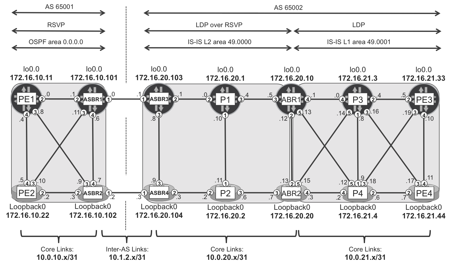
Figure 16-6. Seamless MPLS topology
OSPF, IS-IS, LDP, and RSVP use standard configurations, so let’s concentrate on configuring interdomain LSPs based on BGP-LU.
Going back to the description of LDP tunneling over RSVP (previously in this chapter), a targeted LDP session was established between the endpoints of a RSVP LSP. This targeted LDP session served an important role in facilitating the creation of the end-to-end LDP LSP. It exchanged label bindings in order to “glue” together other LDP LSP segments. These other segments were signaled with hop-by-hop LDP sessions outside the RSVP domain.
There is a powerful analogy between LDP tunneling over RSVP and the Seamless MPLS scenario. BGP-LU also glues together different LSP segments that are built on top of a different underlying technology. There are several types of BGP-LU sessions:
-
BGP-LU sessions established between the endpoints of an underlying intradomain (LDP, RSVP, etc.) LSP. Let’s think of these as targeted sessions.
-
BGP-LU sessions established between directly connected neighbors, if there is no underlying LSP available for tunneling; for example, at the inter-AS border between AS 65001 and AS 65002. Let’s think of these as single-hop (hop-by-hop) sessions.
One major difference compared to LDP tunneling is that you need to configure the BGP-LU sessions manually, whereas targeted LDP sessions were created automatically as a result of the LDP tunneling configuration. On the other hand, LDP tunneling works exclusively over RSVP-TE tunnels, whereas multihop BGP-LU is totally agnostic of the specific intradomain MPLS protocol—it can be LDP, RSVP-TE, SPRING, and so on.
Similar to the LDP tunneling case, in every BGP-LU session, a new MPLS label is allocated and stitched to the label of the previous segment. Whereas in LDP this is automatic, there is a pitfall to avoid in BGP. Very often, the border routers (such as ABR1 and ABR2 in the example topology) act as BGP-LU Route Reflectors (RRs) between domains. It is essential to ensure that every time a border router reflects a BGP-LU route, the BGP next-hop attribute is changed to self: this, in turn, triggers a new label allocation. This is fine because BGP-LU’s purpose is to build transport LSPs.
Note that this recommendation does not apply to service RRs, where changing the BGP next hop is a bad idea. Changing the next-hop on service RRs forces all the upstream traffic in the domain to traverse the RR instead of using the optimal path.
The architecture, showing BGP-LU session structure and hierarchical LSPs in Seamless MPLS designs, is illustrated in Figure 16-7.
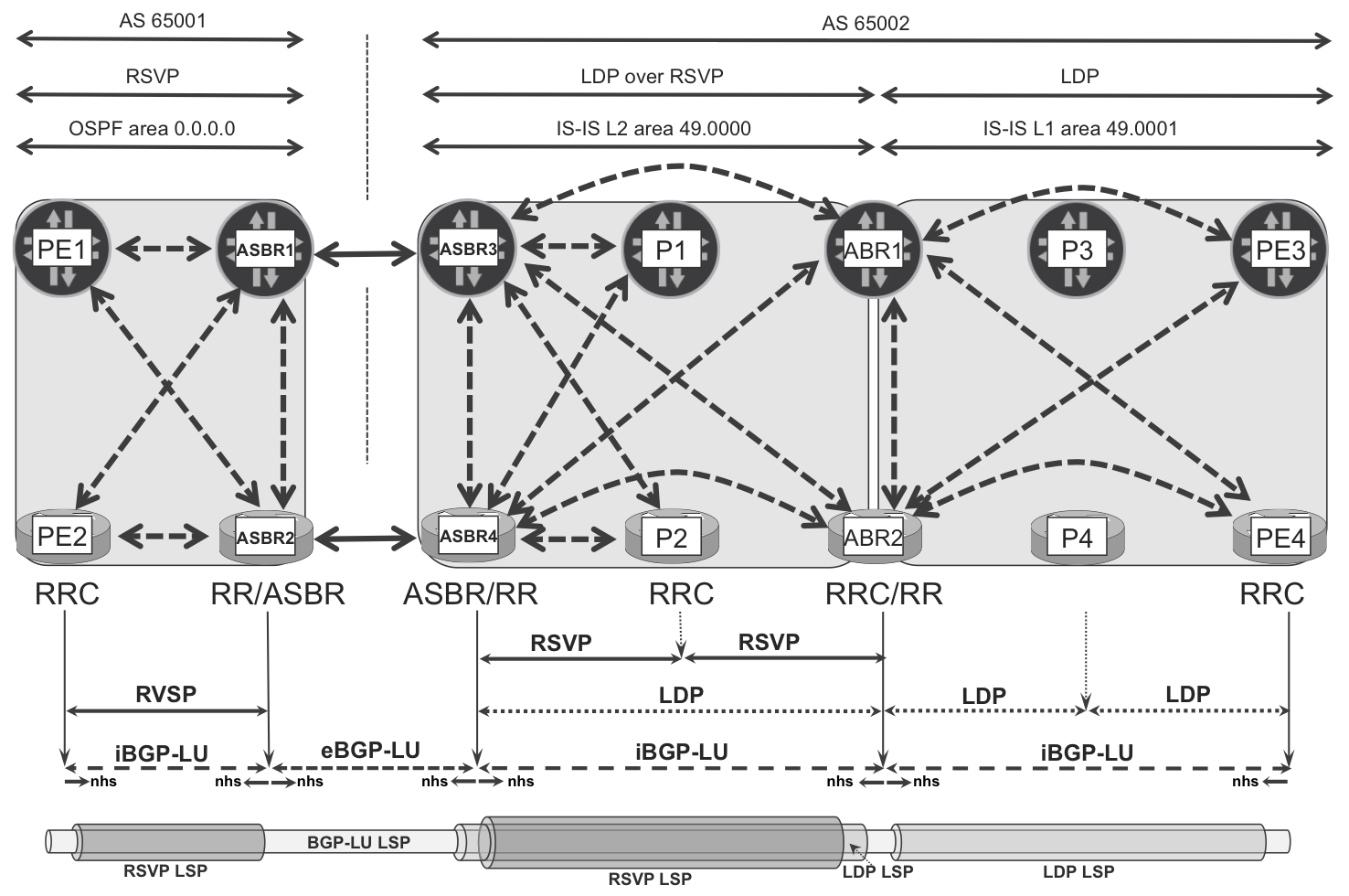
Figure 16-7. BGP-LU architecture for Seamless MPLS
In general, not all the routers participate in the BGP-LU route distribution. For example, routers P3 and P4 do not have any BGP-LU sessions. This illustrates an important fact: the only labeled loopbacks that need to be distributed with BGP-LU correspond to the routers that instantiate the end services (L3VPN, L2VPN, etc.). It also illustrates another fact: routers with limited service capabilities but with sufficient label stack depth can be used as transit nodes. Other loopbacks are not necessarily mapped to labels, unless the administrator wants to run MPLS ping between any two loopbacks in the network for troubleshooting purposes. That having been said, P1 and P2 are included in the BGP-LU distribution; we’ll explain the reason later.
The BGP-LU design is similar to a classical hierarchical RR infrastructure. Four ASBR routers are connected with four BGP sessions in a square: two multihop iBGP sessions between intradomain loopbacks, and two single-hop eBGP sessions between physical link addresses. These ASBRs are at the same time the main BGP-LU RR inside each AS. In AS 65001, there are only two RR clients (RRCs). In AS 65002, however, ASBR3 and ASBR4 have four RRCs: two of them (ABR1 and ABR2) build a second level of RR hierarchy, whose clients are PE3 and PE4. As mentioned earlier, every time a BGP-LU prefix is advertised across a domain (area or AS) boundary, the advertising border router performs a BGP next-hop self action. This is the default behavior on eBGP sessions, but you need to configure it explicitly on iBGP sessions.
The end result, as shown at the bottom of Figure 16-7, is an end-to-end BGP-LU LSP established between PE routers of remote domains. This BGP-LU LSP is tunneled inside the respective intradomain LSPs of each domain, and it is native (not tunneled) on ASBR-ASBR links.
Seamless MPLS—BGP-LU path selection
One important topic related to BGP-LU is the handling of cumulative IGP link metrics. In the case of a MPLS network with a single IGP domain, it’s easy: the IGP calculates end-to-end costs accurately, so the lowest-cost path is selected automatically. In the case of interdomain BGP-LU LSPs, finding the shortest path relies on BGP metric attributes because the IGP cost between IGP domains is not shared across domains.
The standard BGP metric is Multi Exit Discriminator (MED). In principle, one could use MED as the end-to-end cost metric across domains. However, MED has certain limitations that could make large deployments (with many interconnected domains) quite challenging:
-
MED is sent only to a neighboring AS (RFC 4271, Section 5.1.4 - The MULTI_EXIT_DISC attribute received from a neighboring AS MUST NOT be propagated to other neighboring ASes). In a large-scale design with multiple interconnected ASs, the MED might be lost at some place, so the ultimate goal of measuring end-to-end costs in an entire network might be difficult.
-
In the BGP path selection process (RFC 4271, Section 9.1.2.2), the MED is used as a standalone tie-breaking criterion at Step C. The MED takes strict precedence over the IGP metric comparison at Step E. In a BGP-LU–based Seamless MPLS architecture, this is not a good idea.
Let’s illustrate the second bullet point with the example topology. For simplicity, all links have cost 1000, with the exception of three links (as outlined in Figure 16-8), whose IGP metric is temporarily increased to 1500. Also, the diagonal links (PE1-ASBR2, PE2-ASBR1, ABR1-P4, ABR2-P3, P3-PE4, and P4-PE3) are temporarily disabled.
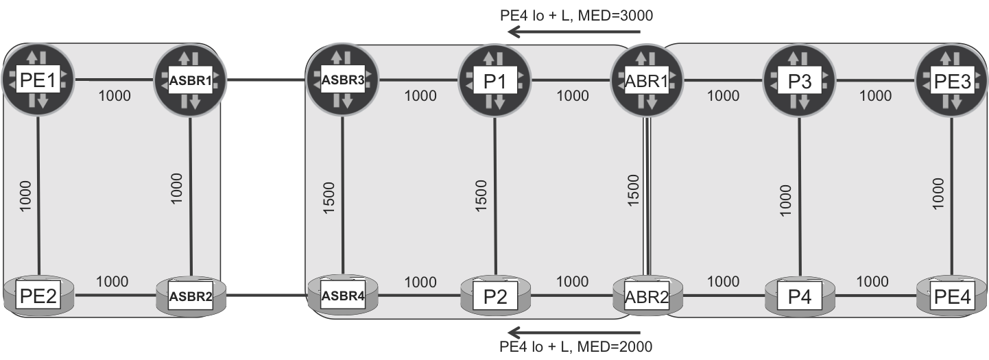
Figure 16-8. BGP-LU MED propagation
Taking into account the cumulative IGP metric, there are multiple possible shortest paths from PE1 to PE4, including these two:
-
PE1→ASBR1→ASBR3→P1→ABR1→P3→PE3→PE4
-
PE1→PE2→ASBR2→ASBR4→P2→ABR2→P4→PE4
The IGP costs in the L1 IS-IS domain are 3000 from ABR1 to PE4, and 2000 from ABR2 to PE4. When the ABRs advertise PE4’s loopback address to the higher-level RRs (ASBR3 and ASBR4), a common practice is to copy the IGP metric into the MED attribute of the BGP-LU route. As a result, ABR1 and ABR2 announce PE4’s loopback with MED values 3000 and 2000, respectively. Following BGP selection rules, both ASBR3 and ASBR4 select the route advertised by ABR2 due to its lower MED value. This makes sense for ASBR4, whose shortest path to PE4 is via ABR2. But it’s not the best option for ASBR3, whose best cumulative IGP metric path is via ABR1.
Even such a simple example shows that using MED in Seamless MPLS scenarios might not be the best choice. To overcome this limitation, RFC 7311 - The Accumulated IGP Metric Attribute for BGP introduces a new BGP attribute called Accumulated IGP cost, or in short, AIGP. This extension to BGP introduces the following behavior:
-
Every time that the BGP next hop (NH) changes, the Accumulated IGP (AIGP) attribute is automatically updated to the value of current_AIGP + IGP_cost_to_current_BGP_NH. This ensures that the total IGP cost across multiple IGP domains is automatically tracked in the AIGP attribute.
-
In the BGP path selection process, among the multiple paths available, the one with a lowest value of current_AIGP + IGP_cost_to_current_BGP_NH wins. This check is performed at the very beginning of the process, even before comparing the AS_PATH attribute length.
Figure 16-9 illustrates the basic principles of AIGP. The BGP-LU prefix (PE4 loopback) is injected initially with AIGP=0. Because the ABR routers change the BGP next hop, they also update the AIGP: ABR1 sets it to 3000, whereas ABR2 sets it to 2000. When ASBR3 receives the updates from ABR1 and ABR2, it performs a path selection using the AIGP logic. ASBR3 compares the value of current_AIGP + IGP_cost_to_current_BGP_NH, chooses the route advertised by ABR1, and propagates it with an updated AIGP value. ASBR4, on the other hand, selects the route advertised by ABR2—again, due to AIGP logic.

Figure 16-9. BGP-LU AIGP propagation
Seamless MPLS—BGP-LU configuration on edge routers (PE1, PE2, PE3, and PE4)
This is the third BGP-LU example in the book. There is a detailed example in Chapter 2 and one more in Chapter 9. For brevity, this section only shows the configuration that is specific to Seamless MPLS as compared to inter-AS Option C.
The first difference is that in the Seamless MPLS architecture some domains are ASs and other domains are IGP areas within a larger AS. BGP is used as a loop-prevention mechanism based on the AS path—if I receive a route with my AS in the AS path, I reject it. Inside an AS there is a similar mechanism based on the cluster list attribute: every iBGP RR adds its cluster ID when it reflects a route and rejects the received routes whose cluster list contains the local cluster ID. Despite the existence of these mechanisms, it is better from a scaling and operational perspective to deploy policies that control the route advertisement flow on the domain borders.
Such policies rely on a geographical community that will eventually help to filter the prefixes based on where the prefix is originally injected.
Example 16-11. Geographical communities
65000:11XYY
    X – autonomous system (1 – 65001, 2 – 65002)
    YY – area (00 – area 0.0.0.0 or 49.0000, 01 – area 49.0001)
For example, PE1 leaks its own loopback from inet.0 to inet.3 with a community called CM-LOOPBACKS-100 (65000:11100). PE1 then announces its local loopback via BGP-LU with this community.
The second difference with respect to inter-AS Option C is that Seamless MPLS uses the AIGP metric attribute in BGP. Putting it all together, following is the delta configuration at PE1:
Example 16-12. Advertising local loopback via BGP-LU on PE1 (Junos)
1     protocols {
2         bgp {
3             group iBGP-RR {
4                 family inet {
5                     labeled-unicast {
6                         aigp;
7                     }
8                 }
9                 export PL-BGP-LU-UP-EXP;
10    }}}
11    policy-options {
12        policy-statement PL-BGP-LU-UP-EXP {
13            term LOCAL-LOOPBACK {
14                from {
15                    protocol direct;
16                    rib inet.3;
17                    community CM-LOOPBACKS-100;
18                }
19                then {
20                    aigp-originate;
21    }}}}
A similar configuration is required on PE3, with the appropriate community.
In the IOS XR configuration shown in Example 16-13, the AIGP attribute is initialized to zero for consistency with Junos. This is the delta configuration for PE2.
Example 16-13. Advertising local loopback via BGP-LU on PE2 (IOS XR)
route-policy PL-BGP-LU-UP-EXP
  if community matches-any CM-LOOPBACKS-100 then
    set aigp-metric 0
    pass
  endif
end-policy
!
router bgp 65001
 neighbor-group iBGP-RR
  address-family ipv4 labeled-unicast
   route-policy PL-BGP-LU-UP-EXP out
!
Let’s look at the receiving side (ASBR2) and verify that the AIGP is correctly set by PE2.
Example 16-14. Received neighbor loopback on ASBR2 (IOS XR)
RP/0/0/CPU0:ASBR2#show bgp 172.16.10.22/32 | begin "Path #1"
 Path #1: Received by speaker 0
 Advertised to peers (in unique update groups):
   10.1.2.3        172.16.10.101
 Local, (Received from a RR-client), (received & used)
   172.16.10.22 (metric 1001) from 172.16.10.22 (172.16.10.22)
     Received Label 3
     Origin incomplete, metric 0, localpref 100, aigp metric 0, [...]
     Community: 65000:11100
     Total AIGP metric 1001
(...)
The Total AIGP metric is 1001, which is the value of the current AIGP (zero) plus the IGP cost (1001) to the next hop (172.16.10.22). The default OSPF metric for a loopback in IOS XR is 1, plus the configured link cost (1000) yields 1001. The Total AIGP metric is used in the BGP path selection process, as discussed earlier. For the sake of completeness, let’s also look at PE2’s BGP-LU route on ASBR1 (Junos).
Example 16-15. Received neighbor loopback on ASBR1 (Junos)
1    juniper@ASBR1> show route receive-protocol bgp 172.16.10.22
2                    table inet.3 detail
3     inet.3: 12 destinations, 25 routes (12 active, 0 holddown, 0 hidden)
4       172.16.10.22/32 (3 entries, 2 announced)
5          Accepted
6          Route Label: 3
7          Nexthop: 172.16.10.22
8          MED: 0
9          Localpref: 100
10         AS path: ?
11         Communities: 65000:11100
12         AIGP: 0
This looks fine, too, although the Total AIGP metric (sum of current AIGP + IGP cost to next hop) is not explicitly displayed in Junos.
Seamless MPLS—BGP-LU configuration on border routers (ASBRs and ABRs)
As already discussed, the ASBR and ABR routers play the role of RRs for BGP-LU prefixes. They perform next-hop self and automatically update the AIGP attribute by taking into account the IGP cost toward the current next hop.
The following design optimizes BGP-LU loopback distribution. This optimization is important in large-scale deployments; otherwise, you can skip it for simplicity.
ASBR1 and ASBR2 have three BGP-LU peer groups, each with a different route policy applied:
-
ASBR1/2 to BGP-LU RRCs (PE1 and PE2) → “DOWN” direction
-
Don’t advertise local loopbacks via BGP-LU, and don’t reflect the loopbacks learned from the local domain back to PE1 and PE2. These prefixes are reachable anyway thanks to the local domain’s IGP/LDP/RSVP protocols.
-
Reflect the BGP-LU loopbacks learned from upstream (eBGP) peers, changing the next hop (configured action) and updating the AIGP (default action).
-
These peers are configured as RR clients (Junos:
cluster, IOS XR:route-reflector-client).
-
-
ASBR1/2 to BGP-LU RR peers (ASBR2 to ASBR1, and the opposite: ASBR1 to ASBR2) → “RR peer” direction
-
Advertise local loopbacks with initial AIGP value (“0”).
-
Reflect the BGP-LU loopbacks learned from upstream (eBGP) peers, changing the next hop (configured action) and updating the AIGP (default action).
-
Reflect other BGP-LU loopbacks, like the ones received from downstream iBGP peers PE1 and PE2, with no attribute (next hop or AIGP) change.
-
-
ASBR1/2 to BGP-LU external peers (ASBR1 to ASBR3, and ASBR2 to ASBR4) → “UP” direction
-
Advertise local loopbacks with initial AIGP value (“0”)
-
Propagate the BGP-LU loopbacks learned from iBGP (downstream or RR) peers, explicitly changing the next hop and updating the AIGP (default action).
-
The configuration is long but has nothing special, just BGP business as usual. Routes can be matched on community, protocol, RIB (Junos), route type (Junos: route-type external, IOS XR: path-type is ebgp), and so on.
The main caveat to be aware of is an implementation difference between Junos and IOS XR in the way the AIGP is handled at the domain border.
Example 16-16 shows the specific BGP-LU configuration at Junos ASBR1.
Example 16-16. BGP-LU policies on ASBR1 (Junos)
1     protocols {
2         bgp {
3             group iBGP-DOWN:LU+VPN {         ## towards PE1 and PE2 (RRC)
4                 family inet {
5                     labeled-unicast { ... }  ## similar config to PE1's
6                 }
7                 export PL-BGP-LU-DOWN-EXP;
8                 cluster 172.16.10.101;
9             }
10            group iBGP-RR:LU+VPN {           ## towards ASBR2 (RR)
11                family inet {
12                    labeled-unicast { ... }
13                }
14                export PL-BGP-LU-RR-EXP;
15            }
16            group eBGP-UP:LU {               ## towards ASBR3 (eBGP)
17                family inet {
18                    labeled-unicast { ... }
19                }
20                export PL-BGP-LU-UP-EXP;
21    }}}
22    policy-options {
23        policy-statement PL-BGP-LU-DOWN-EXP {
24            term 100-LOOPBACKS {
25                from {
26                    protocol [ bgp direct ];
27                    rib inet.3;
28                    community CM-LOOPBACKS-100;
29                }
30                then reject;
31            }
32            term eBGP-LOOPBACKS {
33                from {
34                    protocol bgp;
35                    rib inet.3;
36                    community CM-LOOPBACKS-ALL;
37                    route-type external;
38                }
39                then {
40                    next-hop self;
41                    accept;
42                }
43            }
44            from rib inet.3;
45            then reject;
46        }
47        policy-statement PL-BGP-LU-RR-EXP {
48            term LOCAL-LOOPBACK {
49                from {
50                    protocol direct;
51                    rib inet.3;
52                    community CM-LOOPBACKS-100;
53                }
54                then {
55                    metric 0;
56                    aigp-originate;
57                    next-hop self;
58                    accept;
59                }
60            }
61            term eBGP-LOOPBACKS {
62                from {
63                    protocol bgp;
64                    rib inet.3;
65                    community CM-LOOPBACKS-ALL;
66                    route-type external;
67                }
68                then {
69                    next-hop self;
70                    accept;
71                }
72            }
73            term ALL-LOOPBACKS {
74                from {
75                    protocol [ bgp direct ];
76                    rib inet.3;
77                    community CM-LOOPBACKS-ALL;
78                }
79                then accept;
80            }
81            from rib inet.3;
82            then reject;
83        }
84        policy-statement PL-BGP-LU-UP-EXP {
85            term LOCAL-LOOPBACK {
86                from {
87                    protocol direct;
88                    rib inet.3;
89                    community CM-LOOPBACKS-100;
90                }
91                then {
92                    metric 0;
93                    aigp-originate;
94                    next-hop self;
95                    accept;
96                }
97            }
98            term ALL-LOOPBACKS {
99                from {
100                   protocol bgp;
101                   rib inet.3;
102                   community CM-LOOPBACKS-ALL;
103               }
104               then {
105                   metric 0;
106                   next-hop self;
107                   accept;
108               }
109           }
110           from rib inet.3;
111           then reject;
112       }
113       community CM-LOOPBACKS-100 members 65000:11100;
114       community CM-LOOPBACKS-ALL members 65000:11...;
115   }
Example 16-17 shows the relevant BGP-LU configuration applied to ASBR2.
Example 16-17. BGP-LU policies on ASBR2 (IOS XR)
1     community-set CM-LOOPBACKS-100
2       65000:11100
3     end-set
4     !
5     route-policy PL-BGP-LU-DOWN-EXP
6       if community matches-any (65000:11100) then
7         drop
8       endif
9       if community matches-any (65000:[11000..11999]) then
10        if path-type is ebgp then
11          set next-hop self
12          set aigp-metric + 1
13          done
14        endif
15      endif
16    end-policy
17    !
18    route-policy PL-BGP-LU-RR-EXP
19      if destination in (172.16.10.102/32) then
20        set community CM-LOOPBACKS-100
21        set aigp-metric 0
22        done
23      endif
24      if community matches-any (65000:[11000..11999]) then
25        if path-type is ebgp then
26          set next-hop self
27          set aigp-metric + 1
28          done
29        endif
30        if path-type is ibgp then
31          done
32        endif
33      endif
34    end-policy
35    !
36    route-policy PL-BGP-LU-UP-EXP
37      if destination in (172.16.10.102/32) then
38        set community CM-LOOPBACKS-100
39        set aigp-metric 0
40        set med 0
41        done
42      endif
43      if community matches-any (65000:[11000..11999]) then
44        set med 0
45        done
46      endif
47    end-policy
48    !
49    router bgp 65001
50     bgp router-id 172.16.10.102
51     mpls activate
52      interface GigabitEthernet0/0/0/1
53     !
54     bgp unsafe-ebgp-policy
55     ibgp policy out enforce-modifications
56     address-family ipv4 unicast
57      redistribute connected
58      allocate-label all
59     !
60     neighbor-group iBGP-DOWN:LU_VPN           !! towards PE1 and PE2 (RRC)
61      address-family ipv4 labeled-unicast
62       route-reflector-client
63       route-policy PL-BGP-LU-DOWN-EXP out
64      !
65     !
66     neighbor-group iBGP-RR:LU_VPN             !! towards ASBR1 (RR)
67      address-family ipv4 labeled-unicast
68       route-policy PL-BGP-LU-RR-EXP out
69      !
70     !
71     neighbor-group eBGP-UP:LU                 !! towards ASBR4 (eBGP)
72      address-family ipv4 labeled-unicast
73       aigp
74       send-community-ebgp
75       route-policy PL-BGP-LU-UP-EXP out
76      !
77     !
78    !
79    router static
80     address-family ipv4 unicast
81      10.1.2.3/32 GigabitEthernet0/0/0/1
82     !
83    !
The BGP and policy configurations of ASBR3, ASBR4, ABR1, and ABR2 follow the same principles.
There are some small differences between the default behavior of Junos and IOS XR when it comes to BGP-LU configuration. To unify the overall network behavior, the following measures are taken (in addition to those already mentioned in Chapter 2):
-
AIGP support needs to be explicitly configured for both iBGP and eBGP sessions in Junos (see the syntax in Example 16-12, line 6). In IOS XR, AIGP is enabled by default for iBGP and you need to explicitly configure it for eBGP sessions only (see the syntax on Example 16-17, line 73).
-
An ASBR-to-ASBR link does not have an IGP running. How does the AIGP metric take this link into account? The answer varies across vendors: Junos increases AIGP by default by a value of 1, whereas IOS XR does not alter AIGP when sending BGP updates over such link. To achieve a uniform metric scheme across vendors, the configuration in IOS XR is set to increase the AIGP metric of reflected eBGP prefixes by a value of 1 (see Example 16-17, lines 12 and 27).
-
The manipulation of attributes via outbound route-policies on iBGP sessions is disabled by default in IOS XR, and you need to explicitly enable it (see Example 6-17, line 55).
Seamless MPLS—IPv4 intradomain connectivity between PEs
Now that all the configurations are in place, let’s verify end-to-end LSP connectivity. First, from PE1 to PE4, as demonstrated here:
Example 16-18. BGP-LU Ping from PE1 (Junos) to PE4 (IOS XR)
juniper@PE1> ping mpls bgp 172.16.21.44/32 source 172.16.10.11
!!!!!
--- lsping statistics ---
5 packets transmitted, 5 packets received, 0% packet loss
And now from PE2 to PE3:
Example 16-19. BGP-LU Ping from PE2 (IOS XR) to PE3 (Junos)
RP/0/0/CPU0:PE2#ping mpls ipv4 172.16.21.33/32 fec-type
                bgp source 172.16.10.22
(...)
.....
Success rate is 0 percent (0/5)
Hmm. The MPLS (BGP-LU) ping from Junos to IOS XR across the Seamless MPLS network is fine, but it fails from IOS XR to Junos. This is because the MPLS Echo Reply is a standard UDP over IPv4 packet, and PE3 does not have a route to reach PE2 on its global routing table, as illustrated here:
Example 16-20. Route from PE3 (Junos) to PE2 (IOS XR)
juniper@PE3> show route 172.16.10.22 active-path

inet.3: 14 destinations, 24 routes (14 active, 0 holddown, 0 hidden)
+ = Active Route, - = Last Active, * = Both

172.16.10.22/32
    *[BGP/170] 00:16:15, MED 0, localpref 100, from 172.16.20.10
       AS path: 65001 ?, validation-state: unverified
The route is present, but only in the inet.3 table. As already discussed, the inet.3 table provides BGP next-hop resolution for MPLS-based services, but it is not used for normal packet forwarding. There is no entry in the FIB to forward the IPv4 UDP packet toward PE2, and as a result the forwarding lookup hits the default “reject” entry in the FIB.
Example 16-21. Forwarding entry from PE3 (Junos) to PE2 (IOS XR)
juniper@PE3> show route forwarding-table destination 172.16.10.22/32
             table default
(...)
Destination    Type RtRef Next hop       Type Index    NhRef Netif
default        perm     0                rjct       36     1
To solve the interdomain connectivity problem for regular IP packets in a Seamless MPLS topology, there are two alternative generic solutions:
-
Copying the remote PE’s BGP-LU routes from
inet.3toinet.0. This technique is explained in Chapter 2. -
Alternatively, ABRs can inject into the L1 49.0001 area a default route, or a summary route including the loopbacks of remote PEs. Currently, there is no redistribution or leaking in that sense and the baseline IS-IS configuration in this example is set to explicitly ignore the attached bit.
In large Seamless MPLS networks with up to approximately 100,000 loopbacks, the first option might be applied to devices for which installing all the loopbacks in the FIB is not an issue; the second option should be used for devices with limited FIB capacity.
Let’s see how to configure the second option. The assumption is that PE3 and PE4 are low FIB scale devices, so ABR1 and ABR2 conditionally inject a default route into the 49.0001 area. All the other Junos routers are assumed to be high FIB scale devices that install all the received BGP-LU loopbacks into both inet.3 and inet.0. Example 16-22 and Example 16-23 provide the configuration at ABR1 and ABR2, respectively.
Example 16-22. Conditional default route advertisement on ABR1 (Junos)
routing-options {
    aggregate {
        route 0.0.0.0/0 {
            policy PL-DEFAULT-ROUTE-CONDITION;
            metric 0;
            preference 9;
            discard;
}}}
protocols {
    isis {
        export PL-ISIS-EXP;
}}
policy-options {
    policy-statement PL-DEFAULT-ROUTE-CONDITION {
        term 100-LOOPBACKS {
            from {
                protocol bgp;
                community CM-LOOPBACKS-100;
            }
            then accept;
        }
        then reject;
    }
    policy-statement PL-ISIS-EXP {
        term DEFAULT-ROUTE {
            from {
                protocol aggregate;
                route-filter 0.0.0.0/0 exact;
            }
            to level 1;
            then {
                metric 0;
                accept;
 }}}}
Example 16-23. Conditional default route advertisement on ABR2 (IOS XR)
route-policy PL-DEFAULT-ROUTE-CONDITION
  if rib-has-route in (172.16.10.11/32, 172.16.10.22/32) then
    set level level-1
  endif
end-policy
!
router static
 address-family ipv4 unicast
  0.0.0.0/0 Null0
 !
!
router isis core
 address-family ipv4 unicast
  default-information originate route-policy PL-DEFAULT-ROUTE-CONDITION
In Example 16-22 and Example 16-23, the condition on ABR1 (Junos) is the existence of routes with a specific community, whereas on ABR2 (IOS XR), there is an exact prefix match. In both cases, the ABRs only generate the default route if they have at least one route to one of the loopbacks in AS 65001. For consistency, the Junos configuration explicitly advertises the default route with metric 0, which is the default in IOS XR. The preference of ABR1’s aggregate default route is set to 9, which is lower than the preference of IS-IS routes. Otherwise, the default route from ABR2 would suppress the advertisement from ABR1.
With this configuration in place, PE3 should be able to reach PE2’s loopback via a default route installed both in the inet.0 RIB and in the FIB.
Example 16-24. Route in the RIB of PE3 (Junos) toward PE2 (IOS XR)
juniper@PE3> show route 172.16.10.22 table inet.0

inet.0: 23 destinations, 23 routes (23 active, 0 holddown, 0 hidden)
+ = Active Route, - = Last Active, * = Both

0.0.0.0/0          *[IS-IS/15] 01:20:57, metric 2000
                      to 10.0.21.4 via ge-0/0/2.0
                    > to 10.0.21.18 via ge-0/0/3.0
And, as shown in Example 16-25, the MPLS ping between PE2 and PE3 now works without any problems.
Example 16-25. BGP-LU ping from PE2 (IOS XR) to PE3 (Junos)
RP/0/0/CPU0:PE2#ping mpls ipv4 172.16.21.33/32 fec-type bgp
                source 172.16.10.22
(...)
!!!!!
Success rate is 100 percent (5/5), round-trip min/avg/max = 1/12/30 ms
Services in Seamless MPLS architecture
Now that BGP-LU has built end-to-end transport LSPs through the example topology, it’s time to focus on the end services. Let’s choose IPv4 VPN for illustration purposes. Actually, there are already some BGP sessions established for the exchange of IPv4 labeled unicast prefixes, but can these sessions be reused to signal the IPv4 VPN unicast routes, too? The answer is yes, they can, and if two routers exchange prefixes of both address families directly, there is one BGP session only. But the BGP session layout is different for each address family. To get the complete picture, look at both Figure 16-7 (BGP-LU) and Figure 16-10 (IPv4 VPN).

Figure 16-10. BGP IPv4 VPN unicast in Seamless MPLS architecture
The session layout and the BGP next-hop manipulation for each address family are completely different. This is for a reason: MPLS transport and VPN services are two different worlds, even if the same protocol (BGP) can signal both. The RRs in the IS-IS L2 domain are different for each address family: ASBR3/4 for IPv4 labeled unicast, and P1/2 for IPv4 VPN unicast.
L3VPN in the Seamless MPLS architecture is similar to inter-AS Option C. The most critical aspect is the BGP next-hop handling for each address family:
-
For IPv4 labeled unicast (SAFI=4), the BGP next-hop attribute changes at the border of each domain (area or AS). This provides transport hierarchy, using the local tunneling mechanism of each domain.
-
For IPv4 VPN unicast (SAFI=128), the BGP next hop never changes, as expected with inter-AS Option C. This is the default behavior on iBGP RRs, but it requires a specific configuration on eBGP to preserve the original next-hop value.
No inbound or outbound BGP policies are required for IPv4 VPN. Here are some special configuration requirements:
-
Enabling eBGP multihop between RRs in different ASs
-
Disabling next-hop change on eBGP sessions
-
Disabling the “reject all” default policy of eBGP sessions in IOS XR
-
For BGP sessions that signal both the IPv4 LU and the IPv4 VPN Unicast NLRI (like those represented by double-arrow solid lines in Figure 16-10), ensure that the BGP policy terms treat each address family independently. We discuss this topic in “Multiprotocol BGP policies”.
There is one detail of Figure 16-7 that requires further explanation. P1 and P2 peer with the BGP-LU RRs ASBR3 and ASBR4. From the point of view of end-to-end PE-PE transport LSPs, this is not required: the L2 IS-IS domain has its own tunneling mechanism that is not BGP-LU, and pure P-routers can be completely BGP-free. So why are these sessions configured? The answer is on Figure 16-10: P1 and P2 are the RRs for L3VPN prefixes. Consequently, P1 and P2 need to have reachability to the loopbacks of ASBR1 and ASBR2, and that is why Figure 16-7 shows P1 and P2 as BGP-LU peers.
If P1 and P2 did not participate in BGP-LU distribution, other options would be as follows:
-
Redistributing ASBR1 and ASBR2 loopbacks from BGP-LU into IS-IS at routers ASBR3 and ASBR4
-
ASBR3 and ASBR4 injecting a default route (or a summary route covering ASBR1 and ASBR2 loopbacks) into IS-IS
RRs are a crucial component of the network infrastructure. Using default or summary routes (which suppress more specific routes) to reach these crucial components is considered a bad practice. Redistribution from BGP-LU to IGP is slightly better, but it defeats part of the purpose of using BGP. Thus, the best recommended practice is to include RRs in the BGP-LU delivery mechanism, even if they do not provide VPN services themselves.
The service design model used in this chapter results in all the PE routers receiving all the service prefixes. This approach might not scale for micro-PE (low-scale PE) devices, so Chapter 17 spends more time on optimizing the design.
Multiprotocol BGP policies
In Junos, the following policies evaluate, filter, and modify IP VPN (Unicast) prefixes. It is not mandatory to have all of the policies in place. For example, if there is no local VRF, then there is no vrf-[export|import].
-
For prefix export, the VRF’s
vrf-exportpolicy chain is executed before the globalexportpolicy chain applied to the BGP session (see Example 16-12, line 9, and Example 16-16, lines 7, 14, and 20). You need thevpn-apply-exportknob in order to evaluate the global policy chain. Otherwise, only thevrf-exportpolicy chain (if any) is executed. -
For prefix import, the global import policy chain applied at the BGP session (if any) is executed before the VRF’s
vrf-importpolicy chain (if any).
Note
A policy chain is an ordered sequence of policies. Very often, it consists of one single policy.
-
The IP LU case is simpler: only the global BGP policy chains (applied to the BGP session) evaluate IP LU prefixes.
Here comes the tricky aspect. The same global (import and export) policy chains evaluate both IP LU and IP VPN prefixes. Therefore, you need to carefully define the policy terms so that each term only evaluates prefixes of one address family.
Tip
You can select IP LU prefixes with the condition from rib inet.3. Selecting IP VPN prefixes is trickier, as several RIBs are involved (see Chapter 3 and Chapter 17).
In this Seamless MPLS scenario, the global BGP policies only have to process the IP LU prefixes (in order to change the MED, AIGP, and NH). For this reason, only the from rib inet.3 condition becomes handy. In Chapter 17, you will see an example in which IP VPN prefixes are matched, too.
In IOS XR, policies are applied separately for each address family. Thus, it is easy to keep track of distinct rules that need to be applied to prefixes from different address families. As a result, when multiple address families are deployed, you always need separate policies.
Seamless MPLS—end-to-end forwarding path
Now, after achieving basic connectivity, let’s look at Figure 16-11 and Example 16-26 to understand the label states and operations performed on the IPv4 VPN packets. Note that multiple equal-cost paths exist; therefore, multiple traceroute outputs are possible. ASBR1 was temporarily disabled to reduce the available paths and ensure that the traffic traverses both Junos and IOS XR devices.
Example 16-26. Traceroute from VRF on PE1 (Junos) to PE4 (IOS XR)
juniper@PE1> traceroute routing-instance VRF-A 192.168.1.44
traceroute to 192.168.1.44 (192.168.1.44), 30 hops max, ...
 1  10.0.10.9 (10.0.10.9)  6.919 ms  7.274 ms  5.375 ms
     MPLS Label=16010 CoS=0 TTL=1 S=0
     MPLS Label=16006 CoS=0 TTL=1 S=1
 2  10.1.2.3 (10.1.2.3)  5.781 ms  17.325 ms  6.071 ms
     MPLS Label=16010 CoS=0 TTL=1 S=0
     MPLS Label=16006 CoS=0 TTL=2 S=1
 3  10.0.20.2 (10.0.20.2)  5.988 ms  5.712 ms  5.417 ms
     MPLS Label=16012 CoS=0 TTL=1 S=0
     MPLS Label=16004 CoS=0 TTL=1 S=0
     MPLS Label=16006 CoS=0 TTL=3 S=1
 4  10.0.20.7 (10.0.20.7)  6.037 ms  5.723 ms  5.503 ms
     MPLS Label=16004 CoS=0 TTL=1 S=0
     MPLS Label=16006 CoS=0 TTL=4 S=1
 5  10.0.21.14 (10.0.21.14)  7.514 ms  6.142 ms  7.800 ms
     MPLS Label=301776 CoS=0 TTL=1 S=0
     MPLS Label=16006 CoS=0 TTL=5 S=1
 6  10.0.21.17 (10.0.21.17)  6.020 ms *  7.052 ms
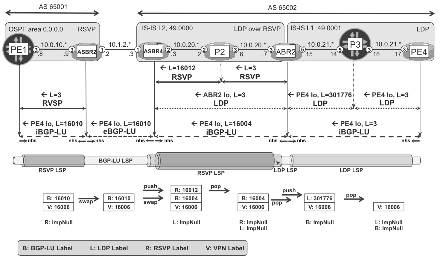
Figure 16-11. MPLS label operations in a Seamless MPLS network
There is label swap operation 16010→16010 at ASBR2. This is totally fine: labels are locally significant and they can have different or the same values.
From the perspective of LDP, the LSP in IS-IS L2 domain of AS 65002 is single hop. If it were multihop, you would see four MPLS labels at this point of the path.
IGP-Less Transport Scaling
Imagine a large-scale data center with more than 100,000 servers in an IGP-less topology (such as the one described in Chapter 2). This data center would require more than 100,000 transport labels to be programmed on the FIB of each device. This is definitely feasible for high-end LSRs, but how about switches with forwarding engines based on merchant silicon? In any case, regardless of the hardware capacity, it is clear that reducing this amount of state would be beneficial. There are at least two complementary strategies to achieve such optimization:
-
Implement a hierarchy between different BGP-LU layers.
-
Take the servers off BGP-LU and use a lighter control plane to program their forwarding plane.
Let’s discuss these two strategies separately.
BGP-LU Hierarchy
As of this writing, this model is not defined in any drafts. It is an original idea by Kaliraj Vairavakkalai, who happens to be one of the key contributors of this book.
So far in this chapter, you have seen the following hierarchical LSP examples: RSVP in RSVP, LDP in RSVP, SPRING in RSVP, and BGP-LU in LDP/RSVP/SPRING. Now it’s the turn of BGP-LU in BGP-LU. Or BGP-LU in BGP-LU in BGP-LU. You can add as many layers as you want to this hierarchy, which is based on a clever manipulation of the BGP-LU routes’ next-hop attribute.
Figure 16-12 is a real lab scenario based on the simplified data center topology from Chapter 2. However, the solution also works on Seamless MPLS scenarios.
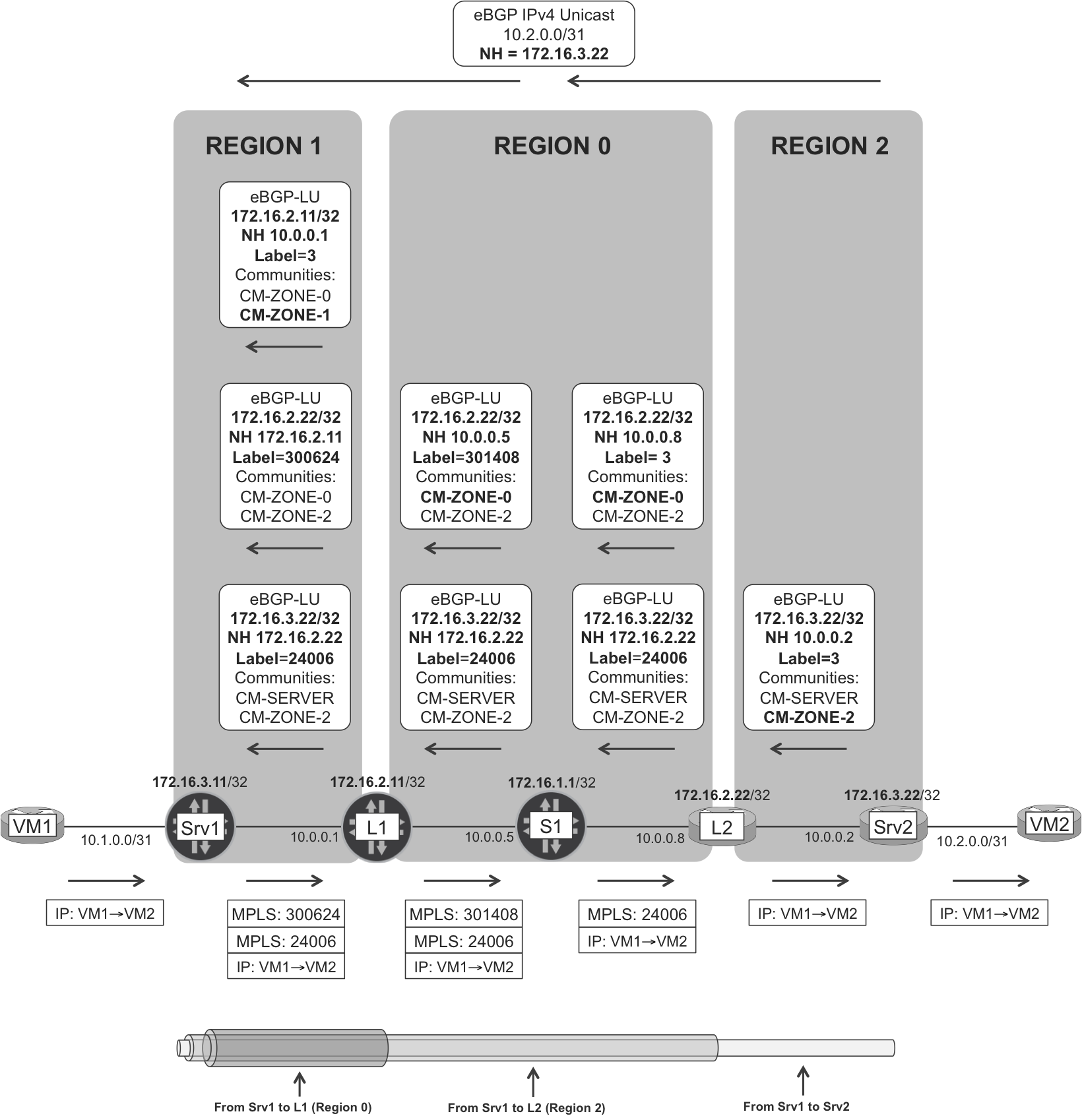
Figure 16-12. BGP-LU hierarchy in IGP-less MPLS network
Note
The key concept is region. A region is basically a part of the network. It can be an IGP area, or an AS, or an AS set.
Indeed, in the IGP-less eBGP scenario illustrated in Figure 16-12 and fully explained in Chapter 2, each router is a different AS. Thus, in this example, any router set is an AS set, and regions typically identify parts of the data center. As you might remember from Chapter 10, modern data center topologies are hierarchical, and it is quite feasible to partition them in regions (e.g., a collection of PODs).
BGP-LU Hierarchy—control plane
With this generalized region concept in mind, the BGP-LU next-hop rewrite rules are as follows:
-
The network is partitioned in regions, and a unique BGP standard community identifies each region.
-
Each router R belongs to a region set, which consists of one or more regions. For example, Srv1’s region set is {1}, whereas L1’s region set is {0,1}.
-
Each region set has an associated regional community set. For example, L1’s regional community set is {CM-ZONE-0, CM-ZONE-1}.
-
When R advertises a non-BGP route (e.g., its own loopback address) into BGP-LU, R is considered to be the originator of the route. R adds to the route all the communities from R’s regional community set.
-
If R has to (re)advertise a BGP-LU route that has at least one community matching R’s regional community set, R considers the route as intraregion. So, R rewrites the route’s BGP next hop of the route to a local address. Which one? It depends on whether the peer is inside or outside the route’s region set. You can extract the rule from Figure 16-12.
-
If R has to (re)advertise a BGP-LU route that has no single community matching R’s regional community set, R considers this route to be interregion. So R does not rewrite the route’s BGP NH.
Note
In summary, only if the route is intraregion, the BGP next hop is rewritten.
Let’s analyze the routes in Figure 16-12 one by one:
- eBGP-LU route 172.16.3.22
- The route is originated by Srv2, whose region set is {2}. Hence, the route has one regional community only: CM-ZONE-2. L2 also belongs to region 2 (and region 0, but this is not important here); hence, it rewrites the BGP next hop of the route to its own loopback address (172.16.2.22) and allocates a locally significant label. Neither of the other routers (S1, L1, Srv1) belongs to region 2, so neither of them touches the BGP next hop or the label.
- eBGP-LU route 172.16.2.22
- The route is originated by L2, whose region set is {0, 2}. As a result, the route has two regional communities: CM-ZONE-0 and CM-ZONE-2. S1 also belongs to region 0; hence, it rewrites the BGP next hop of the route to the eBGP peering address and allocates a locally significant label. L1 also belongs to region 0; hence, it rewrites the BGP of the route to its own loopback address (172.16.2.11) and allocates a new label. As you can see, S1 and L1 followed a different BGP next hop rewrite logic. Indeed, L1 is advertising the route to a peer that, from L1’s perspective, is in region 1. And the route’s region set being {0, 2} does not contain 1 so the route is becoming inter-region.
- eBGP-LU route 172.16.2.11
- Srv1 and L1 are directly connected so this intraregion LSP is very short and has no label due to Penultimate Hop Popping (PHP). If there were another LSR between Srv1 and L1, Srv1 would push a three-label stack just for transport.
Note
The number of BGP routes handled at the control plane is still the same (you could achieve a reduction by using similar techniques to those discussed in Chapter 17).
The scaling benefit of this model is at the FIB or forwarding-plane level. Neither L1 nor S1 need to allocate a label for Srv2’s loopback. In other words, LSRs only allocate labels for prefixes originated in their own region set. So a large-scale data center with more than 100,000 servers no longer requires LSRs to allocate more than 100,000 labels. Allocating a label requires one FIB entry, so the fewer labels that are allocated, the thinner the FIB is.
This example topology is too small to appreciate the real benefits. Think of a network with 1,000 different regions!
Example 16-27 shows the three recursive routes from the perspective of Srv1.
Example 16-27. Hierarchical BGP-LU signaling—Srv1 (Junos)
juniper@Srv1> show route receive-protocol bgp 10.0.0.1
              table inet.3 detail

inet.3: 12 destinations, 12 routes (11 active, ...)
[...]
* 172.16.2.11/32 (1 entry, 1 announced)
     Accepted
     Route Label: 3
     Nexthop: 10.0.0.1
     AS path: 65201 I
     Communities: 65000:1000 65000:1001

* 172.16.2.22/32 (1 entry, 1 announced)
     Accepted
     Route Label: 300624
     Nexthop: 172.16.2.11
     AS path: 65201 65101 65202 ?
     Communities: 65000:1000

* 172.16.3.22/32 (1 entry, 1 announced)
     Accepted
     Route Label: 24006
     Nexthop: 172.16.2.22
     AS path: 65201 65101 65202 65302 ?
     Communities: 65000:3 65000:1002
You can match the routes, next hops, and labels, from Figure 16-12 to Example 16-27. Here are the standard communities in the example:
-
Regional communities: CM-ZONE-X (65000:100X), where X is the region number.
-
Other communities (see Chapter 2): CM-SERVER (65000:3) identifies server loopbacks and CM-VM (65000:100) identifies the end-user virtual machines (VMs).
BGP-LU hierarchy—forwarding plane
As you can see, the hierarchical transport LSP is ready at the ingress PE (Srv1).
Example 16-28. Forwarding next-hop in Hierarchical BGP-LU—Srv1 (Junos)
juniper@Srv1> show route 172.16.3.22 table inet.3

inet.3: 12 destinations, 12 routes (11 active, ...)
[...]
172.16.3.22/32  *[BGP/170] 02:01:28, localpref 10
                   AS path: 65201 65101 65202 65302 ?
                 > to 10.0.0.1 via ge-2/0/2.0,
                                   Push 24006, Push 300624(top)
The MPLS service in this example is global (no VPN) IPv4 unicast. Of course, it could be VPN and that would require yet another (service) label. The service IPv4 unicast route is 10.2.0.0/31, and its BGP next hop (172.16.3.22) has already been resolved, so VM2 is now reachable from VM1. This prefix exchange is depicted on top of Figure 16-12. Please refer to Example 2-11 from Chapter 2 for the layout of BGP sessions distributing service prefixes.
Example 16-29. Forwarding next-hop in Hierarchical BGP-LU—Srv1 (Junos)
juniper@Srv1> show route receive-protocol bgp 172.16.1.1 detail

inet.0: 11 destinations, 11 routes (10 active, ...)
* 10.2.0.0/31 (1 entry, 1 announced)
     Accepted
     Nexthop: 172.16.3.22
     AS path: 65101 65302 ?
     Communities: 65000:100

juniper@Srv1> show route 10.2.0.0/31 table inet.0

inet.0: 11 destinations, 11 routes (10 active, ...)

10.2.0.0/31  *[BGP/170] 00:32:11, localpref 100, from 172.16.1.1
                AS path: 65101 65302 ?
              > to 10.0.0.1 via ge-2/0/2.0,
                                Push 24006, Push 300624(top)

RP/0/0/CPU0:VM#traceroute vrf VM1 10.2.0.1
[...]
 1  10.1.0.0 0 msec  0 msec  0 msec
 2  10.0.0.1 [MPLS: Labels 300624/24006 Exp 0] 29 msec  ...
 3  10.0.0.5 [MPLS: Labels 301408/24006 Exp 0] 0 msec  ...
 4  10.0.0.8 [MPLS: Label 24006 Exp 0] 9 msec  0 msec  ...
 5  10.0.0.2 9 msec  ...
 6  10.2.0.1 9 msec  ...
BGP-LU hierarchy—configuration
You can configure Hierarchical BGP-LU LSPs with plain BGP-LU: no extensions are required. Example 16-30 shows an example of how one eBGP-LU session is configured at L1.
Example 16-30. Hierarchical BGP-LU configuration—L1 (Junos)
1     protocols {
2         bgp {
3             group eBGP-LU-65301 {
4                 multihop {
5                     no-nexthop-change;
6                 }
7                 export PL-eBGP-LU-OUT-REGION-1;
8     }}}
9     policy-options {
10        policy-statement PL-eBGP-LU-OUT-REGION-1 {
11            term LOCAL-LOOPBACK {
12                from interface lo0.0;
13                then {
14                    community add CM-REGION-0;
15                    community add CM-REGION-1;
16                    accept;
17                }
18            }
19            term REGION-0 {
20                from community CM-REGION-0;
21                then {
22                    next-hop 172.16.2.11;
23    }}}
24        community CM-REGION-0 members 65000:1000;
25        community CM-REGION-1 members 65000:1001;
26    }
Note
Junos default BGP policies accept BGP prefixes not already accepted or rejected by any term in the explicit policy (chain) shown in Example 16-30.
The key configuration is on lines 4 and 5:
-
Even if the actual eBGP session is single hop, Junos needs the
multihopstatement in order to set (or accept) the BGP next hop to anything different from the single-hop eBGP peering address. In this example, L1 needs to rewrite the BGP next hop of the 172.16.2.22/32 route to L1’s loopback address 172.16.2.11 before advertising the route to Srv1. -
The
no-nexthop-changeJunos knob means: do not change the BGP NH unless the export policy explicitly changes it. Because this solution requires a mix of rewrites and non-rewrites, the configuration is absolutely required.
As for IOS XR, ebgp-multihop is also required to accept prefixes with a BGP next hop different from the single-hop eBGP peering address. On the other hand, as of this writing, you can configure one single eBGP session in IOS XR in one of these modes: rewrite the next hop of all the prefixes (default) or rewrite the next hop of no prefixes (next-hop-unchanged). The Hierarchical eBGP-LU solution requires a mix of rewrite and non-rewrites, and the authors did not manage to make it work in IOS XR with one single session. IOS XR still supports this solution if you configure two IPv4 addresses on the peering interfaces, establish two parallel eBGP-LU sessions, and carefully use the communities.
MPLS-Capable Servers and Static Labels
Srv1, an MPLS-capable server (acting as a PE) is performing a relatively complex task. Even with hierarchical LSPs, Srv1 still needs to process the eBGP-LU routes of all the remote servers, not to mention the service BGP (IP Unicast, IP VPN, etc.) routes.
Although BGP has many mechanisms to reduce the state (communities, policies RTC, etc.), some large-scale data center administrators prefer to use central controllers that directly program static label stacks on the servers’ FIB.
Note
Of course, eBGP remains the preferred option for the data center fabric (L1, S1, L2, S2, etc.).
For example, if Srv1 does not run eBGP-LU, applying this static configuration to Srv1 would work fine, too, as demonstrated here:
Example 16-31. Static label stack configuration—Srv1 (Junos)
protocols {
    mpls {
        static-label-switched-path Srv1--->Srv2 {
             label-stack;
             ingress {
                 to 172.16.3.22;
                 next-hop 10.0.0.1;
                 push [ 24006 300624 ];
}}}}
The problem is that label values are dynamic and can change at any time. If the controller needs to react every time that a dynamic label value changes in the network, the overall solution does not scale.
There are two alternative ways to solve this challenge:
-
Deterministic labels with BGP-LU Prefix SID extensions (discussed in Chapter 2)
-
Assigning a static label at L1, map it to the FEC 172.16.3.22/32, and push it from Srv1
Static label stitching
Static LSPs like those described in Chapter 1 do not scale, because they require assigning and programming labels at every hop. The following model is better in that the label only needs to be statically allocated at L1. Let’s see how it works.
Example 16-32. Static label stitching configuration at the ingress PE—L1 (Junos)
protocols {
    mpls {
        static-label-switched-path ANY-to-Srv2 {
            transit 1000000 {
                next-hop 172.16.3.22;
                stitch;
}}}}
With this configuration, if L1 receives a MPLS packet with topmost label 1000000, it processes the packet according to how 172.16.3.22 resolves in L1’s inet.3 table. More precisely, the Label Forwarding Information Base (LFIB) entry is: 1000000 → Swap 24006, Push 301408, send to 10.0.0.5.
And if the dynamic labels change, L1 automatically updates the LFIB entry accordingly.
Now suppose that L2 has the following configuration:
Example 16-33. Static label stitching configuration at the egress PE—L2 (IOS XR)
mpls static
 address-family ipv4 unicast
  local-label 1000111 allocate
   forward
    path 1 nexthop GigabitEthernet0/0/0/0 10.0.0.2 out-label pop
!
All that Srv1 needs to do is push label 1000111, then label 1000000, and send the packet to L1. When the packet arrives to L2, it has only one label (1000111) and it is safely delivered to the Srv2.