Chapter 8: Training Models with MLflow
In this chapter, you will learn about creating production-ready training jobs with MLflow. In the bigger scope of things, we will focus on how to move from the training jobs in the notebook environment that we looked at in the early chapters to a standardized format and blueprint to create training jobs.
Specifically, we will look at the following sections in this chapter:
- Creating your training project with MLflow
- Implementing the training job
- Evaluating the model
- Deploying the model in the Model Registry
- Creating a Docker image for your training job
It's time to add to the pyStock machine learning (ML) platform training infrastructure to take proof-of-concept models created in the workbench developed in Chapter 3, Your Data Science Workbench to a Production Environment.
In this chapter, you will be developing a training project that runs periodically or when triggered by a dataset arrival. The main output of the training project is a new model that is generated as output and registered in the Model Registry with different details.
Here is an overview of the training workflow:

Figure 8.1 – Training workflow
Figure 8.1 describes at a high level the general process, whereby a training dataset arrives and a training job kicks in. The training job produces a model that is finally evaluated and deployed in the Model Registry. Systems upstream are now able to deploy inference application programming interfaces (APIs) or batch jobs with the newly deployed model.
Technical requirements
For this chapter, you will need the following prerequisites:
- The latest version of Docker installed on your machine. If you don't already have it installed, please follow the instructions at https://docs.docker.com/get-docker/.
- The latest version of Docker Compose installed—please follow the instructions at https://docs.docker.com/compose/install/.
- Access to Git in the command line, and installed as described at https://git-scm.com/book/en/v2/Getting-Started-Installing-Git.
- Access to a Bash terminal (Linux or Windows).
- Access to a browser.
- Python 3.5+ installed.
- The latest version of your ML library installed locally as described in Chapter 4, Experiment Management in MLflow
Creating your training project with MLflow
You receive a specification from a data scientist based on the XGBoost model being ready to move from a proof-of-concept to a production phase.
We can review the original Jupyter notebook from which the model was registered initially by the data scientist, which is a starting point to start creating an ML engineering pipeline. After initial prototyping and training in the notebook, they are ready to move to production.
Some companies go directly to productionize the notebooks themselves and this is definitely a possibility, but it becomes impossible for the following reasons:
- It's hard to version notebooks.
- It's hard to unit-test the code.
- It's unreliable for long-running tests.
With these three distinct phases, we ensure reproducibility of the training data-generation process and visibility and clear separation of the different steps of the process.
We will start by organizing our MLflow project into steps and creating placeholders for each of the components of the pipeline, as follows:
- Start a new folder in your local machine and name this pystock-training. Add the MLProject file, as follows:
name: pystock_training
conda_env: conda.yaml
entry_points:
main:
data_file: path
command: "python main.py"
train_model:
command: "python train_model.py"
evaluate_model:
command: "python evaluate_model.py "
register_model:
command: "python register_model.py"
- Add the following conda.yaml file:
name: pystock-training
channels:
- defaults
dependencies:
- python=3.8
- numpy
- scipy
- pandas
- cloudpickle
- pip:
- git+git://github.com/mlflow/mlflow
- sklearn
- pandas_datareader
- great-expectations==0.13.15
- pandas-profiling
- xgboost
- You can add now a sample main.py file to the folder to ensure that the basic structure of the project is working, as follows:
import mlflow
import click
import os
def _run(entrypoint, parameters={}, source_version=None, use_cache=True):
print("Launching new run for entrypoint=%s and parameters=%s" % (entrypoint, parameters))
submitted_run = mlflow.run(".", entrypoint, parameters=parameters)
return mlflow.tracking.MlflowClient().get_run(submitted_run.run_id)
@click.command()
def workflow():
with mlflow.start_run(run_name ="pystock-training") as active_run:
mlflow.set_tag("mlflow.runName", "pystock-training")
_run("train_model")
_run("evaluate_model")
_run("register_model")
if __name__=="__main__":
workflow()
- Test the basic structure by running the following command:
mlflow run.
This command will build your project based on the environment created by your conda.yaml file and run the basic project you just created. It should error out, as we need to add the missing files.
At this stage, we have the basic blocks of the MLflow project of the data pipeline that we will be building in this chapter. You will next fill in the Python file to train the data.
Implementing the training job
We will use the training data produced in the previous chapter. The assumption here is that an independent job populates the data pipeline in a specific folder. In the book's GitHub repository, you can look at the data in https://github.com/PacktPublishing/Machine-Learning-Engineering-with-MLflow/blob/master/Chapter08/psystock-training/data/training/data.csv.
We will now create a train_model.py file that will be responsible for loading the training data to fit and produce a model. Test predictions will be produced and persisted in the environment so that other steps of the workflow can use the data to evaluate the model.
The file produced in this section is available at the following link:
https://github.com/PacktPublishing/Machine-Learning-Engineering-with-MLflow/blob/master/Chapter08/psystock-training/train_model.py:
- We will start by importing the relevant packages. In this case, we will need pandas to handle the data, xgboost to run the training algorithm, and—obviously—mlflow to track and log the data run. Here is the code you'll need to do this:
import pandas as pd
import mlflow
import xgboost as xgb
import mlflow.xgboost
from sklearn.model_selection import train_test_split
- Next, you should add a function to execute the split of the data relying on train_test_split from sklearn. Our chosen split is 33/67% for testing and training data respectively. We specify the random_state parameter in order to make the process reproducible, as follows:
def train_test_split_pandas(pandas_df,t_size=0.33,r_state=42):
X=pandas_df.iloc[:,:-1]
Y=pandas_df.iloc[:,-1]
X_train, X_test, y_train, y_test = train_test_split(X, Y, test_size=t_size, random_state=r_state)
return X_train, X_test, y_train, y_test
- This function returns the train and test dataset and the targets for each dataset. We rely on the xgboost matrix xgb.Dmatrix data format to efficiently load the training and testing data and feed the xgboost.train method. The code is illustrated in the following snippet:
if __name__ == "__main__":
THRESHOLD = 0.5
mlflow.xgboost.autolog()
with mlflow.start_run(run_name="train_model") as run:
mlflow.set_tag("mlflow.runName", "train_model")
pandas_df=pd.read_csv("data/training/data.csv")
pandas_df.reset_index(inplace=True)
X_train, X_test, y_train, y_test = train_test_split_pandas(pandas_df)
train_data = xgb.DMatrix(X_train, label=y_train)
test_data = xgb.DMatrix(X_test)
model = xgb.train(dtrain=train_data,params={})
- We also use this moment to produce test predictions using the model.predict method. Some data transformation is executed to discretize the probability of the stock going up or down and transform it into 0 (not going up) or 1 (going up), as follows:
y_probas=model.predict(test_data)
y_preds = [1 if y_proba > THRESHOLD else 0. for y_proba in y_probas]
- As a last step, we will persist the test predictions on the result variable. We drop the index so that the saved pandas DataFrame doesn't include the index when running the result.to_csv command, as follows:
test_prediction_results = pd.DataFrame(data={'y_pred':y_preds,'y_test':y_test})
result = test_prediction_results.reset_index(drop=True)
result.to_csv("data/predictions/test_predictions.csv")
- You can look at your MLflow user interface (UI) by running the following command to see the metrics logged:
mlflow ui
You should be able to look at your MLflow UI, available to view in the following screenshot, where you can see the persisted model and the different model information of the just-trained model:
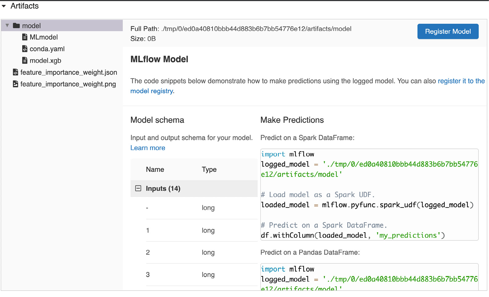
Figure 8.2 – Training model
At this stage, we have our model saved and persisted on the artifacts of our MLflow installation. We will next add a new step to our workflow to produce the metrics of the model just produced.
Evaluating the model
We will now move on to collect evaluation metrics for our model, to add to the metadata of the model.
We will work on the evaluate_model.py file. You can follow along by working in an empty file or by going to https://github.com/PacktPublishing/Machine-Learning-Engineering-with-MLflow/blob/master/Chapter08/psystock-training/evaluate_model.py. Proceed as follows:
- Import the relevant packages—pandas and mlflow—for reading and running the steps, respectively. We will rely on importing a selection of model-evaluation metrics available in sklearn for classification algorithms, as follows:
import pandas as pd
import mlflow
from sklearn.model_selection import train_test_split
from sklearn.metrics import
classification_report,
confusion_matrix,
accuracy_score,
auc,
average_precision_score,
balanced_accuracy_score,
f1_score,
fbeta_score,
hamming_loss,
jaccard_score,
log_loss,
matthews_corrcoef,
precision_score,
recall_score,
zero_one_loss
At this stage, we have imported all the functions we need for the metrics we need to extract in the next section.
- Next, you should add a classification_metrics function to generate metrics based on a df parameter. The assumption is that the DataFrame has two columns: y_pred, which is the target predicted by the training model, and y_test, which is the target present on the training data file. Here is the code you will need:
def classification_metrics(df:None):
metrics={}
metrics["accuracy_score"]=accuracy_score(df["y_pred"], df["y_test"] )
metrics["average_precision_score"]=average_precision_score( df["y_pred"], df["y_test"] )
metrics["f1_score"]=f1_score( df["y_pred"], df["y_test"] )
metrics["jaccard_score"]=jaccard_score( df["y_pred"], df["y_test"] )
metrics["log_loss"]=log_loss( df["y_pred"], df["y_test"] )
metrics["matthews_corrcoef"]=matthews_corrcoef( df["y_pred"], df["y_test"] )
metrics["precision_score"]=precision_score( df["y_pred"], df["y_test"] )
metrics["recall_score"]=recall_score( df["y_pred"], df["y_test"] )
metrics["zero_one_loss"]=zero_one_loss( df["y_pred"], df["y_test"] )
return metrics
The preceding function produces a metrics dictionary based on the predicted values and the test predictions.
- After creating this function that generates the metrics, we need to use start_run, whereby we basically read the prediction test file and run the metrics. We post all the metrics in MLflow by using the mlflow.log_metrics method to log a dictionary of multiple metrics at the same time. The code is illustrated in the following snippet:
if __name__ == "__main__":
with mlflow.start_run(run_name="evaluate_model") as run:
mlflow.set_tag("mlflow.runName", "evaluate_model")
df=pd.read_csv("data/predictions/test_predictions.csv")
metrics = classification_metrics(df)
mlflow.log_metrics(metrics)
- We can look again at the MLflow UI, where we can see the different metrics just persisted. You can view the output here:

Figure 8.3 – Training model metrics persisted
At this stage, we have a model evaluation for our training job, providing metrics and information to model implementers/deployers. We will now move on to the last step of the training process, which is to register the model in the MLflow Model Registry so that it can be deployed in production.
Deploying the model in the Model Registry
Next, you should add the register_model.py function to register the model in the Model Registry.
This is as simple as executing the mlflow.register_model method with the Uniform Resource Identifier (URI) of the model and the name of the model. Basically, a model will be created if it doesn't already exist. If it's already in the registry, a new version will be added, allowing the deployment tools to look at the models and trace the training jobs and metrics. It also allows a decision to be made as to whether to promote the model to production or not. The code you'll need is illustrated in the following snippet:
import mlflow
if __name__ == "__main__":
with mlflow.start_run(run_name="register_model") as run:
mlflow.set_tag("mlflow.runName", "register_model")
model_uri = "runs:/{}/sklearn-model".format(run.info.run_id)
result = mlflow.register_model(model_uri, "training-model-psystock")
In the following screenshot, the registered model is presented, and we can change state and move into staging or production, depending on our workflow:
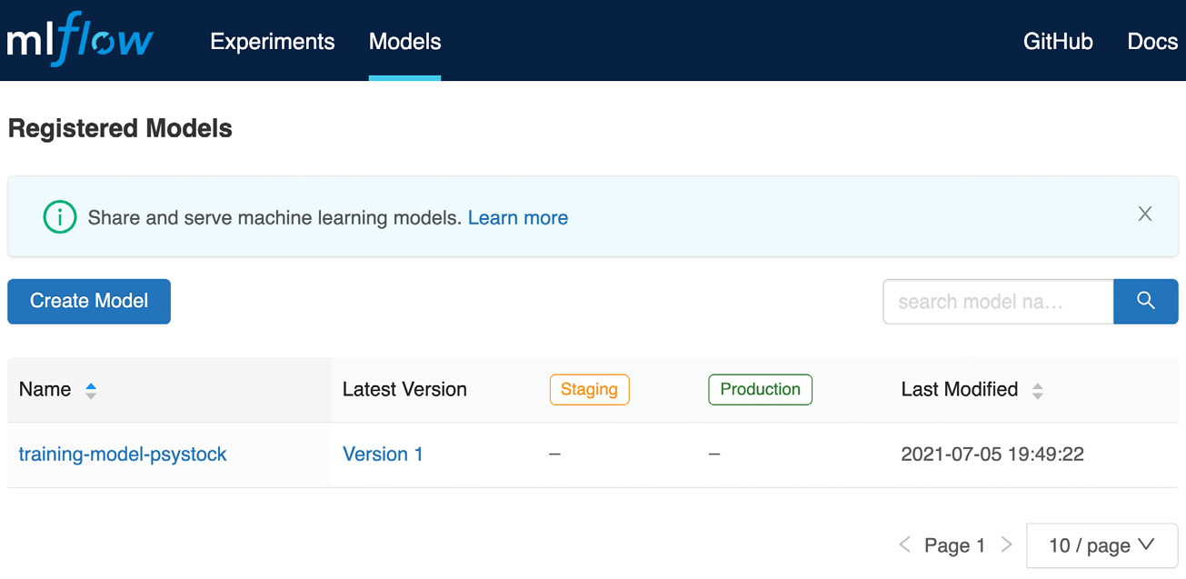
Figure 8.4 – Registered model
After having registered our model, we will now move on to prepare a Docker image of our training job that can be used in a public cloud environment or in a Kubernetes cluster.
Creating a Docker image for your training job
A Docker image is, in many contexts, the most critical deliverable of a model developer to a more specialized systems infrastructure team in production for a training job. The project is contained in the following folder of the repository: https://github.com/PacktPublishing/Machine-Learning-Engineering-with-MLflow/tree/master/Chapter08/psystock-training-docker. In the following steps, we will produce a ready-to-deploy Docker image of the code produced:
- You need to set up a Docker file in the root folder of the project, as shown in the following code snippet:
FROM continuumio/miniconda3:4.9.2
RUN apt-get update && apt-get install build-essential -y
RUN pip install
mlflow==1.18.0
pymysql==1.0.2
boto3
COPY ./training_project /src
WORKDIR /src
- We will start by building and training the image by running the following command:
docker build -t psystock_docker_training_image .
- You can run your image, specifying your tracking server Uniform Resource Locator (URL). If you are using a local address for your MLflow Tracking Server to test the newly created image, you can use the $TRACKING_SERVER_URI value to reach http://host.docker.internal:5000, as illustrated in the following code snippet:
docker run -e MLflow_TRACKING_SERVER=$TRACKING_SERVER_URI psystock_docker_training_image
At this stage, we have concluded all the steps of our complete training workflow. In the next chapter, we will proceed to deploy the different components of the platform in production environments, leveraging all the MLflow projects created so far.
Summary
In this chapter, we introduced the concepts and different features in terms of using MLflow to create production training processes.
We started by setting up the basic blocks of the MLflow training project and followed along throughout the chapter to, in sequence, train a model, evaluate a trained model, and register a trained model. We also delved into the creation of a ready-to-use image for your training job.
This was an important component of the architecture, and it will allow us to build an end-to-end production system for our ML system in production. In the next chapter, we will deploy different components and illustrate the deployment process of models.
Further reading
In order to further your knowledge, you can consult the official documentation at the following link: