Chapter 4: Online Learning with River

In this and the coming three chapters, you will learn how to work with a library for online machine learning called River. Online machine learning is a part of machine learning in which models are designed in such a way that they can update their learned model on the reception of any new data point.

Online machine learning is the opposite of offline machine learning, which is the regular machine learning that you are probably already aware of. In general, in machine learning, a model will try to learn a mathematical rule that can perform a certain task. This task is learned on the basis of a number of data points. The mathematics behind these tasks is based on statistics and algorithmics.

In this chapter, you will discover how to work with online machine learning, and you will discover multiple types of online machine learning. You will go more in depth into the differences between online and offline machine learning. You will also see how to build online machine learning models using River in Python.

This chapter covers the following topics:

• What is online machine learning?
• River for online learning
• A super simple example with River
• A second example with River

Technical requirements

You can find all the code for this book on GitHub at the following link: https://github.com/PacktPublishing/Machine-Learning-for-Streaming-Data-with-Python. If you are not yet familiar with Git and GitHub, the easiest way to download the notebooks and code samples is the following:

1. Go to the link of the repository.
2. Go to the green Code button.
3. Select Download ZIP.

When you download the ZIP file, unzip it in your local environment, and you will be able to access the code through your preferred Python editor.

Python environment

To follow along with this book, you can download the code in the repository and execute it using your preferred Python editor.

If you are not yet familiar with Python environments, I would advise you to check out Anaconda (https://www.anaconda.com/products/individual), which comes with the Jupyter Notebook and JupyterLabs, which are both great for executing notebooks. It also comes with Spyder and VSCode for editing scripts and programs.

If you have difficulty installing Python or the associated programs on your machine, you can check out Google Colab (https://colab.research.google.com/) or Kaggle Notebooks (https://www.kaggle.com/code), which both allow you to run Python code in online notebooks for free, without any setup to do.

Note

The code in the book will generally use Colab and Kaggle notebooks with Python version 3.7.13 and you can set up your own environment to mimic this.

What is online machine learning?

In machine learning, the most common way to train a model is to do a single training pass. The general steps in this approach are as follows:

1. Data preparation.
2. Create a train-test split.
3. Do model benchmarking and hyperparameter tuning.
4. Select the best model.
5. Move this model to production.

This approach is called offline learning.

With streaming data, you can often use this type of model very well. You can build the model once, deploy it, and use it for predicting your input stream. You can probably track the performance metrics of your model, and when the performance starts to change, you can do an update or retraining of your model, deploy the new version, and let it set in the production environment as long as it works.

Online machine learning is a branch of machine learning that contains models that work very differently. They do not learn a full dataset at once, but rather, update the learned model (the decision rules for prediction) through sequential steps. Using such an approach, you can automatically update your model that is in production; it continues to learn on new data.

How is online learning different from regular learning?

The practice of building online learning systems takes a different angle at the machine learning problem than the offline machine learning approach. With offline learning, there is a real possibility to test what a model has learned, whereas, for online learning systems, this can change at any moment.

For some use cases, it is impossible to use offline learning. An example is forecasting use cases. In general, for forecasting, you predict a value in the future. To do so, you use the most recent data available to train and retrain your model. In many forecasting applications, machine learning models are retrained every time a new forecast must be predicted.

Outlier detection is another example where offline learning can be less appropriate. If your model does not integrate each new data point, these data points cannot be used as reference cases against new values. This can be solved through offline learning as well, but online learning may be the more appropriate solution to tackle this use case.

Advantages of online learning

Online learning has two main advantages:

• The first main advantage is that online learning algorithms can be updated. They can, therefore, learn in multiple passes. This way, a big dataset does not have to pass at once in a model but can be passed in multiple steps. This is a big advantage when the datasets are large, or when the computing resources are limited.
• The second advantage of online learning is that an online model can adapt to newer processes when updating: it is less fixed. Therefore, where an offline model can become obsolete when data trends change slightly over time, an online model can adapt to these changes and remain performant.

Challenges of online learning

However, there are also disadvantages to using online learning.

First, the concept is less widespread, and it will be a bit harder to find model implementations and documentation for online learning use cases.

Second, and more important, online learning has a risk of models learning things that you don't want them to learn or things that are wrong. With offline learning, you have much more control to validate what a model learns before pushing it to a production environment, whereas when pushing online learning to production environments, it may well continue to learn and decrease in performance due to the updates that it has learned.

Now that you understand the concept of online learning, let's now discover multiple types of online learning.

Types of online learning

Although there is no clearly defined distinction in types of online machine learning, it is good to consider at least the following three terms: incremental learning, adaptive learning, and reinforcement learning.

Incremental learning

Incremental learning methods are models that can be updated with a single observation at a time. As described previously, one of the main added values of online machine learning is this, as this is something that is not possible with standard offline learning.

Adaptive learning

Just updating the model, however, may not be enough for the second important added value of online learning that was cited before. If you want a model to adapt well to more recent data, you will have to choose an adaptive online learning method. These methods deal well with any situation that would need a model to adapt, for example, new trends that appear in the underlying data before people even become aware of them.

Reinforcement learning

Reinforcement learning is not necessarily considered a subfield of online learning. Although the approach of reinforcement learning is different than the previously cited online learning approaches, it can be used for the same business problems. It is, therefore, important to learn about reinforcement learning as well. It will be covered in more depth in a later chapter. In the coming section, you will see how to use the River package in Python to build online machine learning models.

Using River for online learning

In this section, you will discover the River library for online learning. River is a Python library that is made specifically for online machine learning. Its code base is a result of the combination of the creme and the scikit-multiflow libraries. The goal of River is to become the go-to library for machine learning on streaming data.

In this example, you'll see how to train an online model on a well-known dataset. The steps that you will take throughout this example are the following:

1. Import the data.
2. Reclassify the data to obtain a binary classification problem.
3. Fit an online model for binary classification.
4. Improve the model evaluation using a train-test split.
5. Fit an online multiclass classification model using one-vs-rest.

Training an online model with River

For this example, you will use the well-known iris dataset. You can download it from the UCI machine learning repository, but you can also use the following code to download it directly into pandas.

The steps to get to our goal are as follows:

1. Importing the data
2. Reclassifying the data into a binary problem
3. Converting the data into a suitable input format
4. Learning the model one data point at a time
5. Evaluating the model

We will get started using the following steps:

1. We will first import the dataset as seen here:

Code Block 4-1

#iris dataset classification example

import pandas as pd

colnames = ['sepal_length','sepal_width','petal_length','petal_width','class']

data = pd.read_csv('https://archive.ics.uci.edu/ml/machine-learning-databases/iris/iris.data', names=colnames)

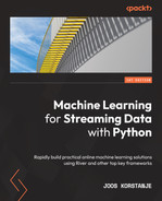
data.head()

The dataset looks as follows:

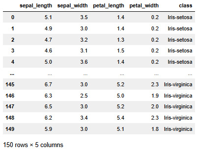
Figure 4.1 – The iris dataset

The iris dataset is very commonly used, mainly in tutorials and examples. The dataset contains a number of observations of three different iris species, a type of flower. For each flower, you have the length and width of specific parts of the plant. You can use the four variables to predict the species of iris.

2. For this first model, you will need to convert the class column into a binary column, as you will use the LogisticRegression model from River, which does not support multiclass:

Code Block 4-2

data['setosa'] = data['class'] == 'Iris-setosa'

data['setosa']

This results in the following output:

Figure 4.2 – The series with Boolean data type

3. As a next step, we will write code to loop through the data to simulate a streaming data input. The X data should be in dictionary format, and y can be string, int, or Boolean. In the following code, you see a loop that stops after the first iteration, so that it prints one X and one y:

Code Block 4-3

# convert to streaming dataset

for i,row in data.sample(1).iterrows():

    X = row[['sepal_length', 'sepal_width', 'petal_length', 'petal_width']]

    X = X.to_dict()

    

    y = row['setosa']

    

    print(X)

    print(y)

    break

You can see that X has to be in a dictionary format, which is relatively uncommon for those who are familiar with offline learning. Then, y can be either Boolean, a string, or an int. This will look as follows:

Figure 4.3 – The x and y inputs for the model

4. Now, let's fit the model one by one. It is important to add .sample(frac=1) to avoid getting the data in order. If you do not add this, the model would first receive all the data from one class and then from the other classes. The model has a hard time dealing with that, so a random order should be introduced using the sample function:

Code Block 4-4

!pip install river

from river import linear_model

model =  linear_model.LogisticRegression()

for i,row in data.sample(frac=1).iterrows():

    X = row[['sepal_length', 'sepal_width', 'petal_length', 'petal_width']]

    X = X.to_dict()

    y = row['setosa']

        

    model.learn_one(X, y)

5. Let's see how the predictions can be made on the training data. You can use predict_many to predict on a data frame, or else you can use predict_one:

Code Block 4-5

preds = model.predict_many(data[['sepal_length', 'sepal_width', 'petal_length', 'petal_width']])

print(preds)

The result looks as follows:

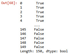
Figure 4.4 – The 150 Boolean observations

6. You can use the scikit-learn accuracy score to estimate the training accuracy of this model:

Code Block 4-6

from sklearn.metrics import accuracy_score

accuracy_score(data['setosa'], preds)

The obtained training accuracy, in this case, is 1, indicating that the model has perfectly learned the training data. Although the model has learned perfect prediction on the data that it has seen during the learning process, it is unlikely that the performance would be as good on new, unseen data points. In the next section, we will improve our model evaluation so that we avoid having overestimated performance metrics.

Improving the model evaluation

In the first example, there was no real relearning and updating.

In this example, we will update and track the accuracy throughout the learning process. You will also see how to keep a training and separate test set. You can use each data point for learning once it arrives, and you will use the updated model for the prediction of the next data point to arrive. This more closely resembles a streaming use case.

The steps to get there are as follows:

1. Train-test split.
2. Fit the model on the training data.
3. Check out the learning curve.
4. Compute performance metrics on the test data.

We will get started as follows:

1. Let's start with a stratified train-test split on the data:

Code Block 4-7

# add a stratified train test split

from sklearn.model_selection import train_test_split

train,test = train_test_split(data, stratify =data['setosa'])

2. You can now redo the same learning loop as before but on the training data. You can see that there is a list called correct to track how the learning has gone over time:

Code Block 4-8

from river import linear_model,metrics

model =  linear_model.LogisticRegression()

correct = []

for i,row in train.sample(frac=1).iterrows():

    X = row[['sepal_length', 'sepal_width', 'petal_length', 'petal_width']]

    X = X.to_dict()

    

    y = row['setosa']

    

    model.predict_one(X)

    correct.append(y == model.predict_one(X))

    

    model.learn_one(X,y)

3. Let's plot the cumulative sum of correct scores over time, to see whether the model learned well from the beginning, or whether the model had fewer errors at the end of the learning curve:

Code Block 4-9

# this model is learning quite stable from the start

import matplotlib.pyplot as plt

import numpy as np

plt.plot(np.cumsum(correct))

You can see that the learning curve is quite linear; the accuracy stays more or less constant over time. It would have been expected to see an improvement in accuracy over time (more correct responses over time, with an exponential-like curve) if the ml was actually improving with training. You can check out the learning curve in the following graph:

Figure 4.5 – The learning curve

4. Finally, let's compute the accuracy on the test score to see how well the model generates out-of-sample data:

Code Block 4-10

# model was not so good on out of sample

accuracy_score(test['setosa'],model.predict_many(test[['sepal_length', 'sepal_width', 'petal_length', 'petal_width']]))

The score that this obtained is 0.94, which is slightly lower than the 1.0 obtained on the train set. This teaches us that the model learned quite well.

In the coming chapters, you'll see more tricks and tools that can help improve models and accuracy.

Building a multiclass classifier using one-vs-rest

In the previous example, you have seen how to build a binary classifier. To do this, you reclassified the target variable into setosa-vs-rest. However, you would want to build one model that allows you to do all of the three classes at the same time. This can be done using River's OneVsRest classifier. Let's now see an example of this:

1. You can start with the same train-test split as before, except that now, you can stratify on the class:

Code Block 4-11

# add a stratified train test split

from sklearn.model_selection import train_test_split

train,test = train_test_split(data, stratify =data['class'])

2. You then fit the model on the training data. The code is almost the same, except that you use OneVsRestClassifier around the call to LogisticRegression:

Code Block 4-12

from river import linear_model,metrics,multiclass

model =  multiclass.OneVsRestClassifier(linear_model.LogisticRegression())

correct = []

for i,row in train.sample(frac=1).iterrows():

    X = row[['sepal_length', 'sepal_width', 'petal_length', 'petal_width']]

    X = X.to_dict()

    

    y = row['class']

    

    model.predict_one(X)

    correct.append(y == model.predict_one(X))

    model.learn_one(X,y)

3. When looking at the learning over time, you can see that the model has started learning better after around 40 observations. Before 40 observations, it had much fewer correct predictions than after:

Code Block 4-13

# this model predicts better after 40 observations

import matplotlib.pyplot as plt

import numpy as np

plt.plot(np.cumsum(correct))

The plot looks as follows. It clearly has a less steep slope in the first 40 observations and accuracy improves after that:

Figure 4.6 – A better learning curve

4. You can again use predict_many to see whether the predictions are any good. When doing predict, you will now not have True/False, but instead, have the string values of each of the iris types:

Code Block 4-14

model.predict_many(test[['sepal_length', 'sepal_width', 'petal_length', 'petal_width']])

This results in the following output:

Figure 4.7 – The multiclass target

5. The test accuracy of the model can be computed using the following code:

Code Block 4-15

# model scores 0.63 on the test data

from sklearn.metrics import accuracy_score

accuracy_score(test['class'],model.predict_many(test[['sepal_length', 'sepal_width', 'petal_length', 'petal_width']]))

The model obtains an accuracy score of 0.63 on the test data.

Summary

In this chapter, you have learned the basics of online machine learning in both theory and practice. You have seen different types of online machine learning, including incremental, adaptive, and reinforcement learning.

You have seen a number of advantages and disadvantages of online machine learning. Among other reasons, you may be almost obliged to refer to online methods if quick relearning is required. A disadvantage is that fewer methods are commonly available, as batch learning remains the industry standard for now.

Finally, you have started practicing and implementing online machine learning through a Python example on the well-known iris dataset.

In the coming chapter, you'll go much deeper into online machine learning, focusing on anomaly detection. You'll see how machine learning can be used to replace the fixed rule alerting system that was built in previous chapters. In the chapters after that, you'll learn more about online classification and regression using River with examples that continue the learnings from the iris classification model from the current chapter.

Further reading

• UCI Machine Learning Repository: https://archive.ics.uci.edu/ml/index.php
• River ML: https://riverml.xyz/latest/
• Online Machine Learning: https://en.wikipedia.org/wiki/Online_machine_learning
• Incremental Learning: https://en.wikipedia.org/wiki/Incremental_learning
• Reinforcement Learning: https://en.wikipedia.org/wiki/Reinforcement_learning
• Logistic Regression: https://www.statisticssolutions.com/free-resources/directory-of-statistical-analyses/what-is-logistic-regression/
• One vs Rest: https://stats.stackexchange.com/questions/167623/understanding-the-one-vs-the-rest-classifier
• Multiclass classification: https://en.wikipedia.org/wiki/Multiclass_classification
• scikit-learn metrics: https://scikit-learn.org/stable/modules/model_evaluation.html