12

Network Data Analysis with Elastic Stack

In Chapter 7, Network Monitoring with Python – Part 1, and Chapter 8, Network Monitoring with Python Part – 2, we discussed the various ways in which we can monitor a network. In the two chapters, we looked at two different approaches for network data collection: we can either retrieve data from network devices such as SNMP or we can listen for the data sent by network devices using flow-based exports. After the data is collected, we will need to store the data in a database, then analyze the data to gain insights in order to decide what the data means. Most of the time, the analyzed results are displayed in a graph, whether that be a line graph, bar graph, or a pie chart. We can use individual tools such as PySNMP, Matplotlib, and Pygal for each of the steps, or we can leverage all-in-one tools such as Cacti or Ntop for monitoring. The tools introduced in those two chapters allowed us to have basic monitoring and understanding of the network.

We then moved on to Chapter 9, Building Network Web Services with Python, to build API services to abstract our network from higher-level tools. In Chapter 10, AWS Cloud Networking, and Chapter 11, Azure Cloud Networking, we extended our on-premises network to the cloud by way of AWS and Azure. We have covered a lot of ground in these chapters and have a solid set of tools to help us make our network programmable.

Starting with this chapter, we will build on our toolsets from previous chapters and look at other tools and projects that I have found useful in my own journey once I was comfortable with the tools covered in previous chapters. In this chapter, we will take a look at an open source project, Elastic Stack (https://www.elastic.co), that can help us with analyzing and monitoring our network beyond what we have seen before.

In this chapter, we will look at the following topics:

• What is the Elastic (or ELK) Stack?
• Elastic Stack installation
• Data ingestion with Logstash
• Data ingestion with Beats
• Search with Elasticsearch
• Data visualization with Kibana

Let's begin by answering the question: what exactly is the Elastic Stack?

What is the Elastic Stack?

The Elastic Stack is also known as the "ELK" Stack. So, what is it? Let's see what the developers have to say in their own words (https://www.elastic.co/what-is/elk-stack):

"ELK" is the acronym for three open source projects: Elasticsearch, Logstash, and Kibana. Elasticsearch is a search and analytics engine. Logstash is a serverside data processing pipeline that ingests data from multiple sources simultaneously, transforms it, and then sends it to a "stash" like Elasticsearch. Kibana lets users visualize data with charts and graphs in Elasticsearch. The Elastic Stack is the next evolution of the ELK Stack.

Figure 1: Elastic Stack (source: https://www.elastic.co/what-is/elk-stack)

As we can see from the statement, the Elastic Stack is really a collection of different projects working together to cover the whole spectrum of data collection, storage, retrieval, analytics, and visualization. What is nice about the stack is that it is tightly integrated but each component can also be used separately. If we do not like Kibana for visualization, we can easily plug in Grafana for the graphs. What if we have other data ingestion tools that we want to use? No problem, we can use the RESTful API to post our data to Elasticsearch. At the center of the stack is Elasticsearch, which is an open source, distributed search engine. The other projects were created to enhance and support the search function. This might sound a bit confusing at first, but as we look deeper at the components of the project, it will become clearer.

We will focus on the network monitoring and data analysis aspects of the Elastic Stack, but the stack has many different use cases including risk management, e-commerce personalization, security analysis, fraud detection, and more. They are being used by a range of organizations; from web companies such as Cisco, Box, and Adobe, to government agencies such as NASA JPL, the United States Census Bureau, and more (https://www.elastic.co/customers/).

Now that we have a better idea of what the ELK Stack is, let's take a look at the lab topology for this chapter.

Lab topology

For the network lab, we will reuse the network topology we used in Chapter 8, Network Monitoring with Python – Part 2. The network gear will have the management interfaces in the 172.16.1.0/24 management network with the interconnections in the 10.0.0.0/8 network and the subnets in /30s.

Where can we install the ELK Stack in the lab? One option is to install the ELK Stack on the management station we have been using up to this point. Another option is to install it on a separate virtual machine (VM) besides the management station with two NICs, one connected to the management network and the other connected to the outside network. My personal preference is to separate the monitoring server from the management server and pick the latter option. The reason for this is that the monitoring server typically has different hardware and software requirements than other servers, as you will see in later sections in this chapter. Another reason for separation is that this setup is more in line with what we will typically see in production; it allows us to separate the management and monitoring between the two servers. Following is a graphical representation of our lab topology:

Figure 2: Lab topology

The ELK Stack will be installed on a new Ubuntu 18.04 server with two NICs, with the first NIC's IP address located in the same management network, 172.16.1.200. The VM will have a second NIC with an IP address of 192.168.2.200 that connects my home network with internet access.

In production, we typically want our ELK cluster to have at least a 3-node system with master and data nodes. In terms of functions, ELK master nodes can control the cluster and index the data while data nodes can perform data-retrieval operations. The 3-node system is recommended for redundancy: 1 node is the active master, while the 2 other nodes are master-eligible if the master node goes down. All three nodes will also be data nodes. We do not need to worry about that for the lab; instead, we will install a 1-node system with a node that is both the master and data node without redundancy.

The hardware requirements for the ELK Stack largely depend on the amount of data we want to put in the system. Since this is a lab, we will not need a lot of horsepower behind the hardware since we will not have a ton of data.

In general, Elasticsearch is more memory-intensive but not as demanding about CPU and storage. We will create a separate VM with the following specifications:

• CPU: 1 vCPU
• Memory: 4 GB (more if possible)
• Disk: 20 GB
• Network: 1 NIC in the lab management network, an (optional) additional NIC for internet access

Elasticsearch is built using Java; each distribution includes a bundle version of OpenJDK. We can download the latest Elasticsearch version from Elastic.co:

echou@elk-stack-mpn:~$ wget https://artifacts.elastic.co/downloads/elasticsearch/elasticsearch-7.4.2-linux-x86_64.tar.gz
echou@elk-stack-mpn:~$ tar -xvzf elasticsearch-7.4.2-linux-x86_64.tar.gz
echou@elk-stack-mpn:~$ cd elasticsearch-7.4.2/

We will need to tweak the default virtual memory settings on the node (https://www.elastic.co/guide/en/elasticsearch/reference/current/vm-max-map-count.html):

echou@elk-stack-mpn:~$ sudo sysctl -w vm.max_map_count=262144

Elasticsearch nodes, by default, will try to discover and form a cluster with other nodes. It is best practice to change the node name and cluster-related items before launching. Let's configure the settings in the elasticsearch.yml file:

echou@elk-stack-mpn:~/elasticsearch-7.4.2$ vim config/elasticsearch.yml
# change the following settings
node.name: mpn-node-1
network.host: <change to your host IP>
http.port: 9200
discovery.seed_hosts: ["mpn-node-1"]
cluster.initial_master_nodes: ["mpn-node-1"]

We can now run Elasticsearch in the background:

echou@elk-stack-mpn:~/elasticsearch-7.4.2$ ./bin/elasticsearch &

We can test the result by performing an HTTP GET request on the host running Elasticsearch this can be done on either the management host or locally on the monitoring host:

(venv) $ curl 192.168.2.200:9200
{
  "name" : "mpn-node-1",
  "cluster_name" : "elasticsearch",
  "cluster_uuid" : "9hTywXc-S9eg3jMi6__XSQ",
  "version" : {
    "number" : "7.4.2",
    "build_flavor" : "default",
    "build_type" : "tar",
    "build_hash" : "2f90bbf7b93631e52bafb59b3b049cb44ec25e96",
    "build_date" : "2019-10-28T20:40:44.881551Z",
    "build_snapshot" : false,
    "lucene_version" : "8.2.0",
    "minimum_wire_compatibility_version" : "6.8.0",
    "minimum_index_compatibility_version" : "6.0.0-beta1"
  },
  "tagline" : "You Know, for Search"
}

Let's repeat this process for the installation of Kibana, our visualization tool:

echou@elk-stack-mpn:~/ $ wget https://artifacts.elastic.co/downloads/kibana/kibana-7.4.2-linux-x86_64.tar.gz
echou@elk-stack-mpn:~/ $ tar -xvzf kibana-7.4.2-linux-x86_64.tar.gz
echou@elk-stack-mpn:~/ $ cd kibana-7.4.2-linux-x86_64/

We'll make some configuration changes in the configuration file as well:

echou@elk-stack-mpn:~/ kibana-7.4.2-linux-x86_64$ vim config/kibana.yml
server.port: 5601
server.host: "192.168.2.200"
server.name: "mastering-python-networking"
elasticsearch.hosts: ["http://192.168.2.200:9200"]

We can start the Kibana process in the background:

echou@elk-stack-mpn:~/kibana-7.4.2-linux-x86_64$ ./bin/kibana &

Once the process has finished launching, we can point our browser to http://<ip address>:5601:

Figure 3: Kibana landing page

We will be presented with an option to load some sample data. This is a great way to get our feet wet with the tool, so let's import this data:

Figure 4: Add Data to Kibana

Great! We are almost done. The last piece of the puzzle is Logstash. Unlike Elasticsearch, the Logstash bundle does not include Java out of the box. We will need to install Java 8 or Java 11 first:

echou@elk-stack-mpn:~$ sudo apt install openjdk-11-jre-headless
echou@elk-stack-mpn:~$ java --version
openjdk 11.0.4 2019-07-16
OpenJDK Runtime Environment (build 11.0.4+11-post-Ubuntu-1ubuntu218.04.3)
OpenJDK 64-Bit Server VM (build 11.0.4+11-post-Ubuntu-1ubuntu218.04.3, mixed mode, sharing)

We can download, extract, and configure Logstash in the same way that we did for Elasticsearch and Kibana:

echou@elk-stack-mpn:~$ wget https://artifacts.elastic.co/downloads/logstash/logstash-7.4.2.tar.gz
echou@elk-stack-mpn:~$ tar -xvzf logstash-7.4.2.tar.gz
echou@elk-stack-mpn:~$ cd logstash-7.4.2/
echou@elk-stack-mpn:~/logstash-7.4.2$ vim config/logstash.yml
node.name: mastering-python-networking
http.host: "192.168.2.200"
http.port: 9600-9700

We will not start Logstash at this time. We'll wait until we have installed the network-related plugins and created the necessary configuration file later in the chapter in order to start the Logstash process.

Let's take a moment to look at deploying the ELK Stack as a hosted service in the next section.

Elastic Stack as a Service

Elasticsearch is a popular service that is available as a hosted option by both Elastic.co and AWS. Elastic Cloud (https://www.elastic.co/cloud/) does not have an infrastructure of its own, but it offers the option to spin up deployments on AWS, Google Cloud Platform, or Azure. Because Elastic Cloud is built on other public cloud VM offerings, the cost will be a bit more than getting it directly from the cloud provider, such as AWS:

Figure 5: Elastic Cloud offerings

AWS offers a hosted Elasticsearch product (https://aws.amazon.com/elasticsearch-service/) that is tightly integrated with the existing AWS offerings. For example, AWS CloudWatch Logs can be streamed directly to the AWS Elasticsearch instance (https://docs.aws.amazon.com/AmazonCloudWatch/latest/logs/CWL_ES_Stream.html):

Figure 6: AWS Elasticsearch service

From my own experience, as attractive as the Elastic Stack is for its advantages, it is a project that I feel is easy to get started but hard to scale without a steep learning curve. The learning curve is even steeper when we do not deal with Elasticsearch on a daily basis. If you, like me, want to take advantage of the features Elastic Stack offers but do not want to become a full-time Elastic engineer, I would highly recommend using one of the hosted options for production.

Which hosted provider to choose depends on your preference of cloud provider lockdown and if you want to use the latest features. Since Elastic Cloud is built by the folks behind the Elastic Stack project, they tend to offer the latest features faster than AWS. On the other hand, if your infrastructure is fully built in the AWS cloud, having a tightly integrated Elasticsearch instance saves you the time and effort required to maintain a separate cluster.

Let's take a look at an end-to-end example from data ingestion to visualization in the next section.

First End-to-End example

One of the most common pieces of feedback from people new to Elastic Stack is the amount of detail you need to understand in order to get started. To get the first usable record in the Elastic Stack, the user needs to build a cluster, allocate master and data nodes, ingest the data, create the index, and manage it via the web or command line interface. Over the years, Elastic Stack has simplified the installation process, improved its documentation, and created sample datasets for new users to get familiar with the tools before using the stack in production.

Before we dig deeper into the different components of the Elastic Stack, it is helpful to look at an example that spans across Logstash, Elasticsearch, and Kibana. By going over this end-to-end example, we will become familiar with the function that each component provides. When we look at each component in more detail later in the chapter, we will be able to compartmentalize where the particular component fits into the overall picture.

Let's start by putting our log data into Logstash. We will configure each of the routers to export the log data to the Logstash server:

r[1-6]#sh run | i logging
logging host 172.16.1.200 vrf Mgmt-intf transport udp port 5144

On our Elastic Stack host, with all of the components installed, we will create a simple Logstash configuration that listens on UDP port 5144 and outputs the data to the Elasticsearch host:

echou@elk-stack-mpn:~$ cd logstash-7.4.2/
echou@elk-stack-mpn:~/logstash-7.4.2$ mkdir network_configs
echou@elk-stack-mpn:~/logstash-7.4.2$ touch network_configs/simple_config.cfg

echou@elk-stack-mpn:~/logstash-7.4.2$ cat network_configs/simple_config.cfg
input {
  udp {
    port => 5144
    type => "syslog-ios"
  }
}

output {
  elasticsearch {
    hosts => ["http://192.168.2.200:9200"]
    index => "cisco-syslog-%{+YYYY.MM.dd}"
  }
}

The configuration file consists of only an input section and an output section without modifying the data. The type, syslog-ios, is a name we picked to identify this index. In the output section, we configure the index name with variables representing today's date. We can run the Logstash process directly from the binary directory in the foreground:

echou@elk-stack-mpn:~/logstash-7.4.2$ sudo bin/logstash -f network_configs/simple_config.cfg
[2019-11-03T09:54:37,201][INFO ][logstash.inputs.udp      ][main] UDP listener started {:address=>"0.0.0.0:5144", :receive_buffer_bytes=>"106496", :queue_size=>"2000"}
<skip>

By default, Elasticsearch allows automatic index generation when data is sent to it. We can generate some log data on the router by resetting the interface, reloading BGP, or simply going into the configuration mode and exiting out. Once there are some new logs generated, we will see the cisco-syslog-<date> index being created:

[2019-11-03T10:01:09,029][INFO ][o.e.c.m.MetaDataCreateIndexService] [mpn-node-1] [cisco-syslog-2019.11.03] creating index, cause [auto(bulk api)], templates [], shards [1]/[1], mappings []
[2019-11-03T10:01:09,130][INFO ][o.e.c.m.MetaDataMappingService] [mpn-node-1] [cisco-syslog-2019.11.03/00NRNwGlRx2OTf_b-qt9SQ] create_mapping [_doc]

At this point, we can do a quick curl to see the index created on Elasticsearch:

(venv) $ curl http://192.168.2.200:9200/_cat/indices/cisco*
yellow open cisco-syslog-2019.11.03 00NRNwGlRx2OTf_b-qt9SQ 1 1 7 0 20.2kb 20.2kb

We can now use Kibana to create the index by going to Settings -> Kibana -> Index Patterns:

Figure 7: Elasticsearch add Index Patterns

Since the index is already in Elasticsearch, we will only need to match the index name. Remember that our index name is a variable based on time; we can use a star wildcard (*) to match all the current and future indices starting with the word Cisco:

Figure 8: Elasticsearch define index pattern

Our index is time-based, that is, we have a field that can be used as a timestamp, and we can search based on time. We should specify the field that we designated as the timestamp. In our case, Elasticsearch was already smart enough to pick a field from our syslog for the timestamp; we just need to choose it in the second step from the drop-down menu:

Figure 9: Elasticsearch configure index pattern timestamp

After the index pattern is created, we can use the Kibana Discover tab to look at the entries visually:

Figure 10: Elasticsearch Index document discovery

After we have collected some more log information, we can stop the Logstash process by using Ctrl + C on the Elastic Stack server. This first example shows how we can leverage the Elastic Stack from data ingestion, to storage, to visualization. The data ingestion used in Logstash (or Beats) is a continuous data stream that automatically flows into Elasticsearch. The Kibana visualization tool provides a way for us to analyze the data in Elasticsearch in a more intuitive way, then create a permanent visualization once we are happy with the result. There are more visualization graphs we can create with Kibana, which we will see more examples of later in the chapter.

Even with just one example, we can see the most important part of the workflow is Elasticsearch. It is the simple RESTful interface, storage scalability, automatic indexing, and quick search result that gives the stack the power to adapt to our network analyzation needs.

In the next section, we will take a look at how we can use Python to interact with Elasticsearch.

Elasticsearch with a Python client

We can interact with Elasticsearch via its HTTP RESTful API using a Python library. For instance, in the following example, we will use the requests library to perform a GET operation to retrieve information from the Elasticsearch host. For example, we know that HTTP GET for the following URL endpoint can retrieve the current indices starting with kibana:

(venv) $ curl http://192.168.2.200:9200/_cat/indices/kibana*
green open kibana_sample_data_ecommerce Pg5I-1d8SIu-LbpUtn67mA 1 0  4675 0    5mb    5mb
green open kibana_sample_data_logs      3Z2JMdk2T5OPEXnke9l5YQ 1 0 14074 0 11.2mb 11.2mb
green open kibana_sample_data_flights   sjIzh4FeQT2icLmXXhkDvA 1 0 13059 0  6.2mb  6.2mb

We can use the requests library to make a similar function in a Python script, Chapter12_1.py:

#!/usr/bin/env python3
import requests

def current_indices_list(es_host, index_prefix):
    current_indices = []
    http_header = {'content-type': 'application/json'}
    response = requests.get(es_host + "/_cat/indices/" + index_prefix + "*", headers=http_header)
    for line in response.text.split('
'):
        if line:
            current_indices.append(line.split()[2])
    return current_indices

if __name__ == "__main__":
    es_host = 'http://192.168.2.200:9200'
    indices_list = current_indices_list(es_host, 'kibana')
    print(indices_list)

Executing the script will give us a list of indices starting with kibana:

(venv) $ python Chapter12_1.py
['kibana_sample_data_ecommerce', 'kibana_sample_data_logs', 'kibana_sample_data_flights']

We can also use the Python Elasticsearch client, https://elasticsearch-py.readthedocs.io/en/master/. It is designed as a thin wrapper around Elasticsearch's RESTful API to allow for maximum flexibility. Let's install it and run a simple example:

(venv) $ pip install elasticsearch

The example, Chapter12_2, simply connects to the Elasticsearch cluster and does a search for anything that matches the indices that start with kibana:

#!/usr/bin/env python3
from elasticsearch import Elasticsearch

es_host = Elasticsearch("http://192.168.2.200/")

res = es_host.search(index="kibana*", body={"query": {"match_all": {}}})
print("Hits Total: " + str(res['hits']['total']['value']))

By default, the result will return the first 10,000 entries:

(venv) $ python Chapter12_2.py
Hits Total: 10000

Using the simple script, the advantage of the client library is not obvious. However, the client library is very helpful when we need to create a more complex search operation such as a scroll where we need to use the return token per query to continue executing the subsequent queries until all the results are returned. The client can also help with more complicated administrative tasks such as when we need to re-index an existing index. We will see more examples using the client library in the remainder of the chapter.

In the next section, we will look at more data ingestion examples from our Cisco device syslogs.

Data ingestion with Logstash

In the last example, we used Logstash to ingest log data from network devices. Let's build on that example and add a few more configuration changes in network_config/config_2.cfg:

input {
  udp {
    port => 5144
    type => "syslog-core"
  }
  udp {
    port => 5145
    type => "syslog-edge"
  }
}
filter {
  if [type] == "syslog-edge" {
    grok {
      match => { "message" => ".*" }
      add_field => [ "received_at", "%{@timestamp}" ]
    }
  }
}
<skip>

In the input section, we will listen on two UDP ports, 5144 and 5145. When the logs are received, we will tag the log entries with either syslog-core or syslog-edge. We will also add a filter section to the configuration to specifically match the syslog-edge type and apply a regular expression section, Grok, for the message section. In this case, we will match everything and add an extra field, received_at, with the value of the timestamp.

We will change r5 and r6 to send syslog information to UDP port 5145:

r[5-6]#sh run | i logging
logging host 172.16.1.200 vrf Mgmt-intf transport udp port 5145

When we start the Logstash server, we will see that both ports are now listening:

echou@elk-stack-mpn:~/logstash-7.4.2$ sudo bin/logstash -f network_configs/config_2.cfg
<skip>
[2019-11-03T15:31:35,480][INFO ][logstash.inputs.udp      ][main] Starting UDP listener {:address=>"0.0.0.0:5145"}
[2019-11-03T15:31:35,493][INFO ][logstash.inputs.udp      ][main] Starting UDP listener {:address=>"0.0.0.0:5144"}
<skip>

By separating out the entries using different types, we can specifically search for the types in the Kibana Discover dashboard:

Figure 11: Syslog Index

If we expand on the entry with the syslog-edge type, we can see the new field that we added:

Figure 12: Syslog timestamp

The Logstash configuration file provides many options in the input, filter, and output. In particular, the filter section provides ways for us to enhance the data by selectively matching the data and further processing it before outputting to Elasticsearch. Logstash can be extended with modules; each module provides a quick end-to-end solution for ingesting data and visualizations with purpose-built dashboards.

Elastic Beats are similar to Logstash modules. They are single-purpose data shippers, usually installed as an agent, that collect data on the host and send the output data either directly to Elasticsearch or to Logstash for further processing.

There are literally hundreds of different downloadable Beats, such as Filebeat, Metricbeat, Packetbeat, Heartbeat, and so on. In the next section, we will see how we can use Filebeat to ingest syslog data into Elasticsearch.

Data ingestion with Beats

As good as Logstash is, the process of data ingestion can get complicated and hard to scale. If we expand on our network log example, we can see that even with just network logs it can get complicated trying to parse different log formats from IOS routers, NXOS routers, ASA firewalls, Meraki wireless controllers, and more. What if we need to ingest log data from Apache web logs, server host health, and security information? What about data formats such as NetFlow, SNMP, and counters? The more data we need to aggregate, the more complicated it can get.

While we cannot completely get away from aggregation and the complexity of data ingestion, the current trend is to move toward a more lightweight, single-purpose agent that sits as close to the data source as possible. For example, we can have a data collection agent installed directly on our Apache server specialized in collecting web log data; or we can have a host that only collects, aggregates, and organizes Cisco IOS logs. Elastic Stack collectively calls these lightweight data shippers Beats: https://www.elastic.co/products/beats.

Filebeat is a version of the Elastic Beats software intended for forwarding and centralizing log data. It looks for the log file we specified in the configuration to be harvested; once it has finished processing, it will send the new log data to an underlying process that aggregates the events and outputs to Elasticsearch. In this section, we will take a look at using Filebeat with the Cisco modules to collect network log data.

Let's install Filebeat and set up the Elasticsearch host with the bundled visualization template and index:

echou@elk-stack-mpn:~$ curl -L -O https://artifacts.elastic.co/downloads/beats/filebeat/filebeat-7.4.2-amd64.deb
echou@elk-stack-mpn:~$ sudo dpkg -i filebeat-7.4.2-amd64.deb

The directory layout can be confusing because they are installed in various /usr, /etc/, and /var locations:

Figure 13: Elastic Filebeat file locations (source: https://www.elastic.co/guide/en/beats/filebeat/7.4/directory-layout.html)

We will make a few changes to the configuration file, /etc/filebeat/filebeat.yml, for the location of Elasticsearch and Kibana:

setup.kibana:
  host: "192.168.2.200:5601"
output.elasticsearch:
  hosts: ["192.168.2.200:9200"]

Filebeat can be used to set up the index templates and example Kibana dashboards:

echou@elk-stack-mpn:~$ sudo filebeat setup --index-management -E output.logstash.enabled=false -E 'output.elasticsearch.hosts=["192.168.2.200:9200"]'
echou@elk-stack-mpn:~$ sudo filebeat setup –dashboards

Let's enable the Cisco module for Filebeat:

echou@elk-stack-mpn:~$ sudo filebeat modules enable cisco

Let's configure the Cisco module for syslog first. The file is located under /etc/filebeat/modules.d/cisco.yml. In our case, I am also specifying a custom log file location:

- module: cisco
  ios:
    enabled: true
    var.input: syslog
    var.syslog_host: 0.0.0.0
    var.syslog_port: 514
    var.paths: ['/home/echou/syslog/my_log.log']

We can start, stop, and check the status of the Filebeat service using the common Ubuntu Linux command, service Filebeat [start|stop|status]:

echou@elk-stack-mpn:~$ sudo service filebeat start

Modify or add UDP port 514 for syslog on our devices. We should be able to see the syslog information under the filebeat-* index search:

Figure 14: Elastic Filebeat index

If we compare that to the previous syslog example, we can see that there are a lot more fields and meta information associated with each record, such as agent.version, event.code, and event.severity:

Figure 15: Elastic Filebeat Cisco log

Why do the extra fields matter? Among other advantages, the fields make search aggregation easier, and this, in turn, allows us to graph the results better. We will see graphing examples in the upcoming section where we discuss Kibana.

Besides the cisco module, there are modules for Palo Alto Networks, AWS, Google Cloud, MongoDB, and many more. The most up-to-date module list can be viewed at https://www.elastic.co/guide/en/beats/filebeat/7.4/filebeat-modules.html.

What if we want to monitor NetFlow data? No problem, there is a module for that! We will run through the same process with the Cisco module by enabling the module and setting up the dashboard:

echou@elk-stack-mpn:~$ sudo filebeat modules enable netflow
echou@elk-stack-mpn:~$ sudo filebeat setup -e

Then, configure the module configuration file, /etc/filebeat/modules.d/netflow.yml:

- module: netflow
  log:
    enabled: true
    var:
      netflow_host: 0.0.0.0
      netflow_port: 2055

We will configure the devices to send the NetFlow data to port 2055. If you need a refresher, please read the relevant configuration in Chapter 8, Network Monitoring with Python – Part 2. We should be able to see the new netflow data input type:

Figure 16: Elastic NetFlow input

Remember that each module came pre-bundled with visualization templates? Not to jump ahead too much into visualization, but if we click on the visualization tab on the left panel, then search for netflow, we can see a few visualizations that were created for us:

Figure 17: Kibana Visualization

Click on the Conversation Partners [Filebeat Netflow] option, which will give us a nice table of the top talkers that we can reorder by each of the fields:

Figure 18: Kibana table

In the next section, we will direct our attention to the Elasticsearch part of the ELK Stack.

Search with Elasticsearch

We need more data in Elasticsearch to make the search and graph more interesting. I would recommend reloading a few of the lab devices to have the log entries for interface resets, BGP and OSPF establishments, as well as device boot up messages. Otherwise, feel free to use the sample data we imported at the beginning of this chapter for this section.

If we look back at the Chapter12_2.py script example, when we did the search, there were two pieces of information that could potentially change from each query; the index and query body. What I typically like to do is to break that information into input variables that I can dynamically change at runtime to separate the logic of the search and the script itself. Let's make a file called query_body_1.json:

{
  "query": {
    "match_all": {}
  }
}

We will create a script, Chapter12_3.py, that uses argparse to take the user input at the command line:

import argparse
parser = argparse.ArgumentParser(description='Elasticsearch Query Options')
parser.add_argument("-i", "--index", help="index to query")
parser.add_argument("-q", "--query", help="query file")

args = parser.parse_args()

We can then use the two input values to construct the search the same way we have done before:

# load elastic index and query body information
query_file = args.query
with open(query_file) as f:
    query_body = json.loads(f.read())

# Elasticsearch instance
es = Elasticsearch(['http://192.168.2.200:9200'])

# Query both index and put into dictionary
index = args.index
res = es.search(index=index, body=query_body)
print(res['hits']['total']['value'])

We can use the help option to see what arguments should be supplied with the script. Here are the results when we use the same query against the two different indices we created:

(venv) $ python3 Chapter12_3.py --help
usage: Chapter12_3.py [-h] [-i INDEX] [-q QUERY]

Elasticsearch Query Options

optional arguments:
  -h, --help            show this help message and exit
  -i INDEX, --index INDEX
                        index to query
  -q QUERY, --query QUERY
                        query file
(venv) $ python3 Chapter12_3.py -q query_body_1.json -i "cisco*"
50
(venv) $ python3 Chapter12_3.py -q query_body_1.json -i "filebeat*"
10000

When we are developing our search, it usually takes a few tries before we get the result we are looking for. One of the tools Kibana provides is a developer console that allows us to play around with the search criteria and view the search results on the same page. For example, in the following figure, we execute the same search we have done now and we're able to see the returned JSON result. This is one of my favorite tools on the Kibana interface:

Figure 19: Kibana Dev Tools

Much of the network data is based on time, such as the log and NetFlow data we have collected. The values are taken at a snapshot in time, and we will likely group the value in a time scope. For example, we might want to know "who are the NetFlow top talkers in the last 7 days?" or "which device has the most BGP reset messages in the last hour?" Most of these questions have to do with aggregation and time scope. Let's look at a query that limits the time range, query_body_2.json:

{
  "query": {
    "bool": {
    "filter": [
      {
        "range": {
          "@timestamp": {
            "gte": "now-10m"
          }
        }
      }
    ]
    }
  }
}

This is a Boolean query, https://www.elastic.co/guide/en/elasticsearch/reference/current/query-dsl-bool-query.html, which means it can take a combination of other queries. In our query, we use the filter to limit the time range to be the last 10 minutes. We copy the Chapter12_3.py script to Chapter12_4.py and modify the output to grab the number of hits as well as loop over the actual returned results list.

<skip>
res = es.search(index=index, body=query_body)
print("Total hits: " + str(res['hits']['total']['value']))
for hit in res['hits']['hits']:
    pprint(hit)

Executing the script will show that we only have 68 hits in the last 10 minutes:

(venv) $ python3 Chapter12_4.py -i "filebeat*" -q query_body_2.json
Total hits: 68

We can add another filter option in the query to limit the source IP via query_body_3.json:

{
  "query": {
    "bool": {
      "must": {
        "term": {
          "source.ip": "192.168.0.1"
        }
      },
<skip>

The result will be limited by both the source IP of r1's loopback IP in the last 10 minutes:

(venv) $ python3 Chapter12_4.py -i "filebeat*" -q query_body_3.json
Total hits: 18

Let's modify the search body one more time to add an aggregation, https://www.elastic.co/guide/en/elasticsearch/reference/current/search-aggregations-bucket.html, that takes a sum of all the network bytes from our previous search:

{
  "aggs": {
        "network_bytes_sum": {
          "sum": {
            "field": "network.bytes"
        }
    }
  },
  <skip>
}

The result will be different every time we run the script, Chapter12_5.py. The current result is about 1 MB for me when I run the script consecutively:

(venv) $ python3 Chapter12_5.py -i "filebeat*" -q query_body_4.json
1089.0
(venv) $ python3 Chapter12_5.py -i "filebeat*" -q query_body_4.json
990.0

As you can see, building a search query is an iterative process; you typically start with a wide net and gradually narrow the criteria to fine-tune the results. In the beginning, you will probably spend a lot of time reading the documentation and searching for the exact syntax and filters. As you gain more experience under your belt, the search syntax will become easier. Going back to the previous visualization we saw from the netflow module setup for the NetFlow top talker, we can use the inspection tool to see the Request body:

Figure 20: Kibana request

We can put that into a query JSON file, query_body_5.json, and execute it with the Chapter12_6.py file. We will receive the raw data that the graph was based on:

(venv) $ python3 Chapter12_6.py -i "filebeat*" -q query_body_5.json
{'1': {'value': 8156040.0}, 'doc_count': 8256, 'key': '10.0.0.5'}
{'1': {'value': 4747596.0}, 'doc_count': 103, 'key': '172.16.1.124'}
{'1': {'value': 3290688.0}, 'doc_count': 8256, 'key': '10.0.0.9'}
{'1': {'value': 576446.0}, 'doc_count': 8302, 'key': '192.168.0.2'}
{'1': {'value': 576213.0}, 'doc_count': 8197, 'key': '192.168.0.1'}
{'1': {'value': 575332.0}, 'doc_count': 8216, 'key': '192.168.0.3'}
{'1': {'value': 433260.0}, 'doc_count': 6547, 'key': '192.168.0.5'}
{'1': {'value': 431820.0}, 'doc_count': 6436, 'key': '192.168.0.4'}

In the next section, let's take a deeper look at the visualization part of the Elastic Stack: Kibana.

Data visualization with Kibana

So far, we have used Kibana to discover data, manage indices in Elasticsearch, use developer tools to develop queries, and use a few other features. We also saw the pre-populated visualization charts from NetFlow, which gave us the top talker pair from our data. In this section, we will walk through the steps of creating our own graphs. We will start by creating a pie chart.

A pie chart is great at visualizing a portion of the component in relation to the whole. Let's create a pie chart based on the Filebeat index that graphs the top 10 source IP addresses based on the number of record counts. We will select Visualization -> New Visualization -> Pie:

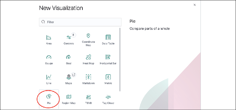
Figure 21: Kibana pie chart

Then we will type netflow in the search bar to pick our [Filebeat NetFlow] indices:

Figure 22: Kibana pie chart source

By default, we are given the total count of all the records in the default time range. The time range can be dynamically changed:

Figure 23: Kibana time range

We can assign a custom label for the graph:

Figure 24: Kibana chart label

Let's click on the Add option to add more buckets. We will choose to split the slices, pick the terms for aggregation, and select the source.ip field from the drop-down menu. We will leave the option for descending but increase the size to 10.

The change will only be applied when you click on the apply button at the top. It is a common mistake to expect the change to happen in real time when using a modern website and not by clicking on the apply button:

Figure 25: Kibana play button

We can click on the Options link at the top to turn off Donut and turn on Show labels:

Figure 26: Kibana chart options

The final graph is a nice pie chart showing the top IP sources based on the number of document counts:

Figure 27: Kibana pie chart

As with Elasticsearch, the Kibana graph is also an iterative process that typically takes a few tries to get right. What if we split the result into different charts instead of slices on the same chart? Yeah, that is not very visually appealing:

Figure 28: Kibana split chart

Let's stick to splitting things into slices on the same pie chart and change the time range to the Last 1 hour, then save the chart so that we can come back to it later.

Note that we can also share the graph either in an embedded URL (if Kibana is accessible from a shared location) or a snapshot:

Figure 29: Kibana save chart

We can also do more with the metrics operations. For example, we can pick the data table chart type and repeat our previous bucket breakdown with the source IP. But we can also add a second metric by adding up the total number of network bytes per bucket:

Figure 30: Kibana metrics

The result is a table showing both the number of document counts as well as the sum of the network bytes. This can be downloaded in CSV format for local storage:

Figure 31: Kibana tables

Kibana is a very powerful visualization tool in the Elastic Stack. We are just scratching the surface of its visualization capabilities. Besides many other graph options to better tell the story of your data, we can also group multiple visualizations onto a dashboard to be displayed. We can also use Timelion (https://www.elastic.co/guide/en/kibana/7.4/timelion.html) to group independent data sources for a single visualization, or use Canvas (https://www.elastic.co/guide/en/kibana/current/canvas.html) as a presentation tool based on data in Elasticsearch.

Kibana is typically used at the end of the workflow to present our data in a meaningful way. We have covered the basic workflow from data ingestion to storage, retrieval, and visualization in the span of a chapter. It still amazes me that we can accomplish so much in a short span of time with the aid of an integrated, open source stack such as Elastic Stack.

Summary

In this chapter, we used the Elastic Stack to ingest, analyze, and visualize network data. We used Logstash and Beats to ingest the network syslog and NetFlow data. Then we used Elasticsearch to index and categorize the data for easier retrieval. Finally, we use Kibana to visualize the data. We used Python to interact with the stack and help us gain more insights into our data. Together, Logstash, Beats, Elasticsearch, and Kibana present a powerful all-in-one project that can help us understand our data better.

In the next chapter, we will look at using Git for network development with Python.