
1
Nonlinear Corrector for CFD
This chapter examines methods for improving an already obtained numerical solution with a reasonable computational effort. In the case of a Poisson problem, two types of approaches are identified. First, the corrector can rely on an a priori estimate. Second, the corrector can rely on a fictitious computation on a twice finer mesh through the defect correction (DC) process. A nonlinear version is the central point in the discussion. The description of nonlinear methods is focused on the Reynolds-averaged Navier–Stokes (RANS) equations. Examples of applications are RANS computations around airfoil and wing and the Euler evaluation of a supersonic flow around low-boom aircraft.
1.1. Introduction
The numerical simulation of engineering problems involves a discrete solution, which is alleged to converge toward the continuous solution of the problem as the size of the elements of the mesh decreases. As the exact solution of the continuous problem is sought, the difference between the numerical and the analytical solution is often seen as an unavoidable noise. But in an engineering context, this error can have disastrous consequences on the numerical prediction which can, in turn, lead to actual accidents or misconceptions (Collins et al. 1997; Jakobsen and Rosendahl 1994; Feghaly et al. 2008). It is thus essential not only to reduce but also to estimate this error. This is usually done by applying a mesh convergence study, see the previous chapter and Oberkampf and Trucano (2002), where the error is estimated with the difference between two solutions computed on two successive meshes. However, this approach is valid only if the asymptotic mesh-convergence has already been reached and requires an additional finer mesh (and thus expensive) calculation in order to appropriately estimate the error of the current solution. A mesh convergence study is thus mandatory to have a reasonable confidence into the discrete outputs, but it may fail. For instance, the AIAA CFD prediction workshops (Rumsey et al. 2011; Levy et al. 2017; Rumsey and Slotnick 2015; Tinoco et al. 2017) have pointed out the dependency of the results on the type of meshes used, since two families of meshes may lead to two different answers. In consequence, very strict meshing guidelines based on previous experiences1 are provided to minimize this effect, but this increases substantially the time required to generate meshes that meet these guidelines. Estimations of the error are based on the fact that the discrete solution Wh does not satisfy the continuous problem Ψ(W) = 0 or on the fact that a projection of the exact solution W on the discrete space does not satisfy the discrete problem Ψh(Wh) = 0 either. This can be stated in a priori and a posteriori ways:
where ΠhW is a discrete projection of the continuous field W and Wh is the discrete solution. Notation Ψ holds for the differential operator defining the equation we are solving and Ψh is the discretization of Ψ. The idea behind correction is to use these defect equations [1.1] or [1.2] in order to estimate a corrector δWh, which can be added to the first solution to get a corrected solution ![]() :
:
which should be sufficiently closer to the exact solution than W or to its projection ΠhW.
In the a priori case we write it formally as follows:
The difference ΠhW − Wh can be approximated if we have a method to approximate Ψh(ΠhW). It is explained in section 1.2.2.
In the a posteriori case, we write formally (considering that W = Wh + δWh):
The evaluation of Ψ(Wh) is a delicate task. An insufficiently accurate evaluation results in useless corrector δWh. A robust option is to approximate the continuous residual Ψ(Wh) by a discrete residual Ψh/2(Wh) computed on a two times finer mesh. The rest of this section focuses on the a priori approach with this second option.
1.1.1. Linear correction
Corrections have been addressed by different means in the past with the dual weighted residual (DWR) method (Becker and Rannacher 1996; Giles and Suli 2002a; Venditti and Darmofal 2002; Jones et al. 2006; Leicht and Hartmann 2010; Fidkowski and Darmofal 2011), and more generally the goal-oriented method (Loseille et al. 2010b) and the error transport equations (ETEs) (Layton et al. 2002; Pierce and Giles 2004; Hay and Visonneau 2006; Derlaga and Park 2017). DWR/goal-oriented methods focus on the correction of a functional. In some cases, the corrected functional is a higher order approximation of it. ETE methods focus on solution fields. Both rely on the same principles. As concerns DWR/goal-oriented methods, the linearization of the functional reads
Since the projection ΠhW is unknown, we introduce a finer mesh h/2. Put directly, we have
In our standpoint, computing the fine-grid solution Wh/2 for evaluating a corrector is too costly. Conversely, knowing Wh, the evaluation of Ψh/2(Πh/2Wh) is affordable, and we have
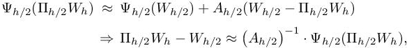
where  is the Jacobian of Ψh/2. From relations [1.4] and [1.5], we obtain
where ![]() is the adjoint of the problem. In order to avoid the computation and the inversion of the large matrix Ah/2, the functional j and the numerical system are assumed to have a similar behavior on coarser and finer meshes so that
is the adjoint of the problem. In order to avoid the computation and the inversion of the large matrix Ah/2, the functional j and the numerical system are assumed to have a similar behavior on coarser and finer meshes so that ![]() is replaced by Wh, its analog on h:
is replaced by Wh, its analog on h:
Then, the RHS is a corrected approximation of jh(Wh), which is obtained with the extra evaluation of the adjoint state ![]() and the finer grid residual
and the finer grid residual ![]() .
.
Similarly, the ETE method computes the corrected solution field from the linearization of the problem as
where ![]() is a defect residual obtained by different reconstruction means to estimate the error introduced by the discretization. The linearization of the problem is a determining factor for the quality of the corrected solution (Yan and Gooch 2015; Yan and Ollivier-Gooch 2017). This is true for both approaches. In particular, an approximate Jacobian obtained by passing to a lower spatial order of accuracy (as used in the Navier–Stokes solver introduced in Chapter 1) should not be used as it will lead to a poor correction. Lastly, would the computation of the matrix
is a defect residual obtained by different reconstruction means to estimate the error introduced by the discretization. The linearization of the problem is a determining factor for the quality of the corrected solution (Yan and Gooch 2015; Yan and Ollivier-Gooch 2017). This is true for both approaches. In particular, an approximate Jacobian obtained by passing to a lower spatial order of accuracy (as used in the Navier–Stokes solver introduced in Chapter 1) should not be used as it will lead to a poor correction. Lastly, would the computation of the matrix  even be exact, these two approaches are limited by the fact that the residual is linearized.
1.1.2. Nonlinear correction
Let us consider the ETE iteration with a RHS evaluated on a finer grid:
where ![]() is a transfer from finer grid h/2 to grid h. If the updating
is a transfer from finer grid h/2 to grid h. If the updating ![]() can be reiterated and converged, we can gain the following advantages:
can be reiterated and converged, we can gain the following advantages:
– the implementation is simple when we already have a Jacobian;
– it does not require a more accurate approximate Jacobian than the one of the flow solver;
– it automatically takes into account all numerical features and nonlinearities of the solver (limiter, flux reconstruction, Riemann solver, etc.).
This chapter is organized as follows. We first discuss in section 1.2 two ways of defining correctors for the usual P1 approximation of a Poisson problem. We then recall in section 1.3 the notations related to the RANS equations and to their discretization. In section 1.4, the nonlinear discrete corrector for that scheme is explained. In section 1.5, we show the application of the finite volume nonlinear corrector to an inviscid supersonic flow simulation for a Sonic Boom prediction workshop.
1.2. Two correctors for the Poisson problem
1.2.1. Notations
Let ![]() Ω being a sufficiently smooth computational domain of
Ω being a sufficiently smooth computational domain of ![]() . The continuous PDE system is written as
. The continuous PDE system is written as
where
and where ![]() is a positive, possibly discontinuous, scalar field in
is a positive, possibly discontinuous, scalar field in ![]() Further, we assume that the bilinear form a is coercive in space V , that is, there exists a positive α such that
Further, we assume that the bilinear form a is coercive in space V , that is, there exists a positive α such that
This model exemplifies the pressure equation in some multi-phase incompressible flow formulation for which mesh adaptation is useful (e.g. Guégan et al. 2010). Let Ωh =Ω for simplicity, τh a triangulation of Ωh and Vh be the usual P1 -continuous finite-element approximation space related to τh:
The finite-element discretization of [1.6] is written in variational and operational form:
in such a way that uh is a linear function of fh, which we denote ![]() .We denote by Πh the usual interpolation operator:
.We denote by Πh the usual interpolation operator:
Scalar correctors, that is, correctors for scalar outputs j(uh) depending on the solution, for example, j(uh)= (g, uh) with g prescribed, have been defined by Giles and Pierce (1999). Our interest concerns the correction of the unknown field itself. Two options are now proposed.
1.2.2. A priori corrector for the PDE solution
A first rather simple a priori corrector can be derived from an analysis of the error RHS. We observe that:
Assuming that the solution u is continuous, we can apply to u the usual P1 interpolator Πh and get:
We call ![]() the implicit error. By implicit, we mean that it can be obtained through solving a discrete system. It differs from the approximation error by an interpolation error:
the implicit error. By implicit, we mean that it can be obtained through solving a discrete system. It differs from the approximation error by an interpolation error:
In order to find an approximate of the implicit error, we need to evaluate the RHS of [1.8] for any test function φh. The second term of RHS of [1.8] is easy to evaluate (we know f and fh). The first term of RHS of [1.8] can be transformed as follows (assuming that ![]() is constant on each element):
is constant on each element):
Then, we get
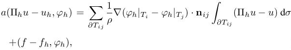
where the sum is taken for all edges ∂Tij separating triangles Ti and Tj of the triangulation. The unit vector nij normal to ∂Tij is pointing outward Ti.Now, we do not know u but uh. In order to evaluate the interpolation error, we first approximate the Hessian of u by an approximation Hh(uh) in Vh of the Hessian of uh. We apply the recovery method of Zienkiewicz-Zhu type (1992) described in section 5.4.3 of Volume 1. This produces the values at vertices of the approximate Hessian Hh(uh). Then, Πhu − u is approximated by the continuous interpolation error πhuh − uh defined in section 5.4.6 of Volume 1. This P2 by element function is zero at vertices and ![]() at mid-edges ij. We apply the same type of estimate to f − fh, namely,
at mid-edges ij. We apply the same type of estimate to f − fh, namely, ![]() In order to approximate the implicit error Πhu − uh, solution of [1.10], we define our a priori implicit corrector as follows:
In order to approximate the implicit error Πhu − uh, solution of [1.10], we define our a priori implicit corrector as follows:
This corrector is an approximation of Πhu − uh. Replacing again the unknown interpolation error by its evaluation on the discrete approximation, we define our a priori corrector as follows:
Assuming that the approximations made between [1.10] and [1.11] are small, the a priori corrector ![]() is then built in such a way that (formally)
is then built in such a way that (formally)
This corrector is easy to compute, but we shall see in Chapter 6 of this volume that its accuracy is rather low.
1.2.3. Finer-grid DC corrector for the PDE solution
A second option relies on using a fictitious finer grid. Here, we write it in the linear case. Let us assume that the approximation is in its asymptotic mesh convergence phase for the mesh Ωh under study of size h. Then, this will be also true for a strictly two times finer embedding mesh Ωh/2 and, for our second-order accurate scheme applied to a sufficiently smooth problem, the heuristics of Richardson analysis is written as
where uh and uh/2 are, respectively, the solutions on Ωh and Ωh/2. Note that in the case of local singularities, second-order convergence [1.13] is not true for uniform meshes since global convergence degrades to first-order convergence. But Chapter 2 of Volume 1 tends to show that it holds almost everywhere for a sequence of adapted meshes (see also Loseille et al. 2007).
Then, at least formally, we have
which implies
Now,
where Ph→h/2 linearly interpolates coarse values on fine mesh. This allows to evaluate Πhu − uh but needs to solve a finer grid system. Let us introduce the residual transfer Rh/2→h, which accumulates on coarser grid vertices the values at finer vertices in neighboring coarse elements multiplied with barycentric weights. In order to reduce the computational cost to solving a coarser grid system, we approximate ![]() by
by ![]()
This motivates the definition of a finer grid DC corrector as follows:
The DC corrector ![]() approximates Πhu − uh instead of u − uh and can be corrected as the previous one:
approximates Πhu − uh instead of u − uh and can be corrected as the previous one:
1.3. RANS equations
1.3.1. Vector form of the RANS system
The compressible Navier–Stokes equations for mass, momentum and energy conservation with Spalart–Allmaras turbulence model are those described in Chapter 1 of Volume 1. It is useful to re-write the RANS system in the following more compact vector form:

(+ boundary conditions), where ![]() (idem for S). W is the non-dimensionalized conservative variables vector:
(idem for S). W is the non-dimensionalized conservative variables vector:
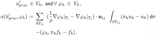
![]() are the convective (Euler) flux functions:
are the convective (Euler) flux functions:
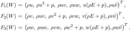
S(W) = (S1(W),S2(W), S3(W)) are the viscous fluxes:
where Tij are the components of laminar stress tensor ![]()
![]() :
:
Q(W) are the source terms, that is, the diffusion, production and destruction terms from the Spalart–Allmaras turbulence model:
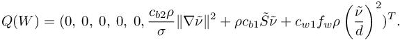
Note that Q = 0 in the case of the laminar Navier–Stokes equations, additional source terms are added (to take into account gravity, for instance).
1.3.2. Formal discretization
1.3.2.1. Finite element discretization
In the standard Galerkin (possibly stabilized) approach, the strong form of the equations over a given domain Ω is reshaped in a weak form:
with additional boundary conditions and where V (Ω) = ![]() =
= ![]() is the functional space in which the solution is sought. The problem is discretized by restricting the functional space to a subset Vh(Ω) of V (Ω). In the standard finite element approach, the domain Ω is split in a finite number of discrete elements Ki (triangles, tetrahedra, hexahedra, prisms, etc.) on which the restriction φh|Ki is a polynomial for each function φh ∈ Vh(Ω) and so that ∪iKi =Ω. The value of φh|Ki on each element is determined by a set of given nodal values and the functions φi – defined by setting the ith node to 1 and the other to 0 – form a basis of Vh(Ω). The residual vector of the discrete problem is defined by
is the functional space in which the solution is sought. The problem is discretized by restricting the functional space to a subset Vh(Ω) of V (Ω). In the standard finite element approach, the domain Ω is split in a finite number of discrete elements Ki (triangles, tetrahedra, hexahedra, prisms, etc.) on which the restriction φh|Ki is a polynomial for each function φh ∈ Vh(Ω) and so that ∪iKi =Ω. The value of φh|Ki on each element is determined by a set of given nodal values and the functions φi – defined by setting the ith node to 1 and the other to 0 – form a basis of Vh(Ω). The residual vector of the discrete problem is defined by
1.3.2.2. Finite volume discretization
In the standard finite volume approach, the domain Ω is split in a finite number of cells ∪iCi = Ω and the residual is defined as
for any continuous field W, where Ci is the cell associated with vertex Pi. The problem is discretized defining the vector Wi = ∫C WdΩ, supposed to be the mean value of the field on each cell, and a reconstructioni operator U that recovers a field W on each cell from the discrete values Wi. For flow problems, the advection terms can be written as a divergence; thus using the Green formulae, the integral of advection term is the integral of the advection fluxes over the boundaries of the cell:
where n is the inward normal and U a reconstruction operator that recovers a field W on each cell from the discrete values Wh.
1.3.3. Notations for discretization
The spatial discretization of the RANS model is described in Chapter 1 of Volume 1. We give here some details of the implementation of our in-house finite volume– finite element flow solver Wolf as this induces several constraints – as we will see – on the implementation of the corrector. In the sequel, we denote for a given vertex Pi:
– E(Pi) the set of edges joining Pi to another vertex Pj of the mesh;
– V1(Pi) the set of vertices that are neighbors of Pi, that is, the set of vertices connected to Pi by an edge. V1(Pi) is named the first-order ball of Pi.
– V2(Pi) the set of vertices that are neighbors of the neighbors of Pi. V2(Pi) is named the second-order ball of Pi. Similarly, Vk(Pi) is the kth iteration of this process.
The discretization of Euler fluxes are sufficiently described in Chapter 1 of Volume 1. Concerning the viscous terms using the P1 finite element method (FEM), we use the following notations:
where ∂Cij is the common interface between cells Ci and Cj . Let φi be the P1 finite element basis function associated with vertex Pi, we have
and as the solution is represented on the P1 basis, S(Wi) (which comes from a gradient) is assumed constant by parts on each element K, for example,
where μ|K is the mean value of μ on the element to be constant. Then, we obtain
The effective computation of the previous integral then leads to the computation of integrals of the following form:
In this expression, ∇φi|K is the constant gradient of basis function φi associated with vertex Pi. In the facts, these terms are computed element-wise and each contribution is added to each vertex of the element. Given an element K =(Pi,Pj , Pk, Pl), we have the partial flux associated with each vertex:
1.4. Nonlinear functional correction
1.4.1. Finite volume nonlinear corrector
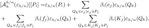
The central idea is to approximate Ψ(Wh) by Ψh/n(Wh). To accumulate on the h-mesh the residual computed on the h/n-mesh, we split the accumulation process depending on the possible configurations. If we consider a h-mesh vertex Pi, for the accumulation of the residual at Pi the different cases are as follows:
– the h/n-mesh vertex Qk coincides with the h-mesh vertex Pi, then the full residual is accumulated: εh/n(Qk) = εh/n(Pi);
– the h/n-mesh vertex Qk belongs to a h-mesh edge ej containing Pi, then we compute the barycentric coordinates βi(ej ) of Qk w.r.t. Pi on edge ej (Alauzet 2016). The accumulated residual is βi(ej )εh/n(Qk);
– the h/n-mesh vertex Qk belongs to a h-mesh face fj containing Pi, then we compute the barycentric coordinates βi(fj ) of Qk with respect to Pi on face fj . The accumulated residual is βi(fj )εh/n(Qk );
– the h/n-mesh vertex Qk is inside a h-mesh element Kj containing Pi, then we compute the barycentric coordinates βi(Kj ) of Qk with respect to Pi in element Kj . The accumulated residual is βi(Kj )εh/n(Qk).
For the h-mesh vertex Pi, the accumulation process is expressed as
For n = 2, this gives Algorithm 1.1. A 2D example of this accumulation process at the element level is illustrated in Figure 1.1.
Applying the NS solver to compute (1) the initial solution, (2) the residual on the h/2-mesh and (3) the corrected solution ensure that the corrector encompasses all the features of the solver (extrapolation, Riemann solver, limiters etc.). The number of iterations required to compute the corrected solution depends on the considered problem (essentially its nonlinearity), the simplified Jacobian and the linear solver used (preconditioner and fixed point iteration) in case of incomplete linear convergence. As the initial and the corrected solution are relatively close to each other, the number of iterations required to compute the corrected solution is typically about 1/10 to 1/100 of the number of iterations required to compute the initial solution. Finer subdivision (h/4, h/8, etc.) of the initial mesh can also be used to improve the predictions. It is very important to note that linearly interpolating the discrete solution Wh on the h/2-mesh (i.e. using Πh/2(Wh)) is nonetheless convenient but also essential to the precision of the correction. Replacing Πh/2(Wh) by a better polynomial reconstruction tends to reduce the efficiency of the correction. Indeed, as we want to quantify the error of piecewise linear solution Wh with respect to the h/2-mesh; it is counter productive to try to improve Πh/2(Wh). More numerical implementation details are given in Frazza et al. (2019).
Algorithm 1.1. Finite volume nonlinear corrector computation
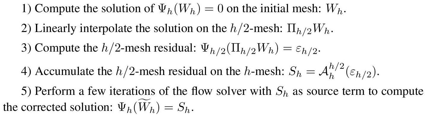
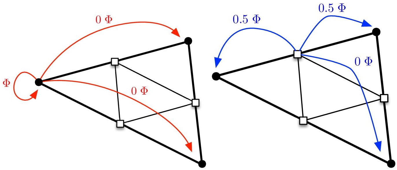
Figure 1.1. Examples of linear accumulation process when the h/2-mesh vertex Qk coincides with the h-mesh vertex Pi (left) and when the h/2-mesh vertex Qk is the mid-point of a h-mesh edge e (right). For a color version of this figure, see www.iste.co.uk/dervieux/meshadaptation2
1.4.2. Finite element corrector
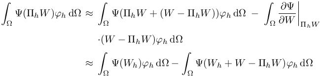
We transpose the variational derivation of section 1.2.2:
In particular, the exact solution verifies
but generally
We have

and by linearizing the fluxes in ΠhW and Wh, we have

and
From these three relations above, we deduce for all φh ∈ Vh:
This expression relies on the fact that Wh is relatively close to ΠhW, so that the derivatives  are approximatively the same. It has two major advantages. First, it does not require to compute the derivative
  , which saves a lot of trouble: as we mentioned previously, in linear approaches, the quality of the correction depends on the choice and the precision of these derivatives. Second, it automatically takes into well of the residual. As long as the higher derivatives
  the nonlinearitiesare relatively close, which is a reasonable assumption as the correction
 ![]() is a purely local correction, the Taylor developments mentioned previously can be expanded.
is a purely local correction, the Taylor developments mentioned previously can be expanded.
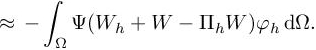
In relation [1.21], we still need to estimate W − ΠhW that represents a loss of smoothness due to the discretization of the solution; it does not depend on the absolute value of the solution but on its variations. The term W+ W − ΠhW can be thus estimated by reconstructing a smooth solution ![]() (Clément 1975; Zienkiewicz and Zhu 1992; Bank and Smith 1993) from the actual numerical solution Wh as shown in Figure 1.2. Finally, the source term can be expressed as
(Clément 1975; Zienkiewicz and Zhu 1992; Bank and Smith 1993) from the actual numerical solution Wh as shown in Figure 1.2. Finally, the source term can be expressed as

where Uk+1 holds for the (k +1)th order reconstruction if the solution is of order k. We propose Algorithm 1.2. to compute the corrector. Note that there is no need for a finer mesh in this case as the integrals are computed on the same elements, but more quadrature points are required to have a consistent computation of the source term given by relation [1.22].
Algorithm 1.2. Finite element nonlinear corrector computation
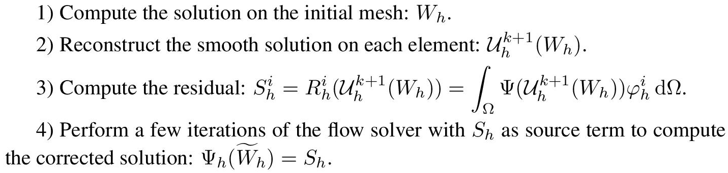
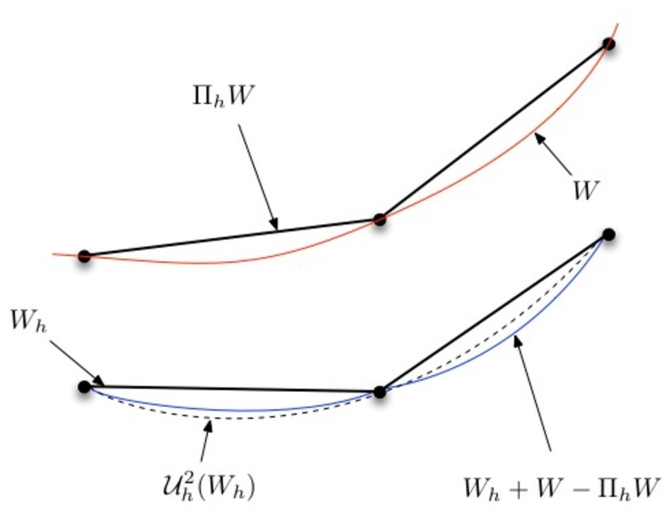
Figure 1.2. Reconstruction of a smoother solution (dashed curve) from a discrete solution (straight segments) compared to the exact solution (W) and the reconstructed solution with the exact defect (Wh + W − ΠhW). For a color version of this figure, see www.iste.co.uk/dervieux/meshadaptation2
REMARK 1.1.– For both nonlinear corrector methods, we take great care to propose methods that do not require any additional memory costs. With regard to the computational cost, the computation of the source term Sh is approximatively the cost of one flow solver iteration, which is negligible.
1.5. Example: supersonic flow
In Frazza et al. (2019), the interested reader will find, among others, numerical experiments with manufactured solutions. We shall stress here the interest of the corrector by giving a short view of a computation described in details in Frazza et al. (2019). The considered flow (C25D Euler flow) is one among those proposed for the 2nd AIAA Sonic Boom prediction workshop (Park and Nemec 2017). An idea of the geometry and the resulting flow is given in Figure 1.3. Figure 1.4 (left) shows the pressure signatures (normalized pressure difference with the free stream pressure) under the aircraft at a distance2 R/L = 1, computed on the tailored meshes provided for the workshop. Error bars represent the estimated error of each nodal value computed with the nonlinear corrector. We can see that the corrector indicates that the error level remains relatively high, even on the 13 million vertices mesh. This has been confirmed by the workshop results: the solution mesh convergence is not achieved on the provided series of tailored meshes. This is visible on the leading shock, which is still relatively smooth, and the shocks in the aft part of the signature (65 < X < 80), which are still forming. Note that the actual subdivision by two of the size of this mesh with 13 million vertices would have yielded a mesh with 104 millions vertices! Figure 1.4 (right) shows the same computations using the goal-oriented mesh adaptation of Chapter 4 of this volume, where the goal is to optimally capture the integral of pressure signature. We can see that the error bars are much smaller. This is especially visible on the mid-part of the signature (50 < X < 60). It is even more enlightening to compare the error levels predicted by the corrector on the tailored workshop mesh composed of 13 million vertices in the mid-part of the signature to the actual difference between the solutions on the tailored mesh and adapted mesh composed of 5.9 million vertices. The error predicted by the corrector on tailored mesh matches the difference between the solution on the tailored mesh (which is not converged) and the solution on the adapted mesh (which is converged in this region).
The results obtained by the corrector (and presented in more detail in Loseille et al. 2018) are interesting because they are, in particular, pointing out a large error in the aft-part of the pressure signature (65 < X < 80) on the workshop tailored meshes, while this error does not appear with adequately adapted meshes.
1.6. Concluding remarks
This chapter presents nonlinear correctors for the finite volume and the finite element methods, which are based either on a local subdivision of the mesh, or a local reconstruction of the solution, and an extra-resolution of the problem with an added source term. The main advantages of this strategy are as follows:
– we need not solve the problem on the global subdivided mesh or at a higher order that yields large memory overhead and is unsuitable when dealing with realistic cases. The proposed methods do not require any additional memory costs;
– the local subdivision makes it easy to parallelize the computation of the source term;
– the cost of computing the nonlinear corrector is usually less than 10% of the overall simulation cost;
– the corrector automatically takes into account the nonlinearities of the problem at hand because we perform many iterations of the flow solver with the added source term to compute the corrected solution;
– the corrected solution takes into account all the features of the considered numerical method.
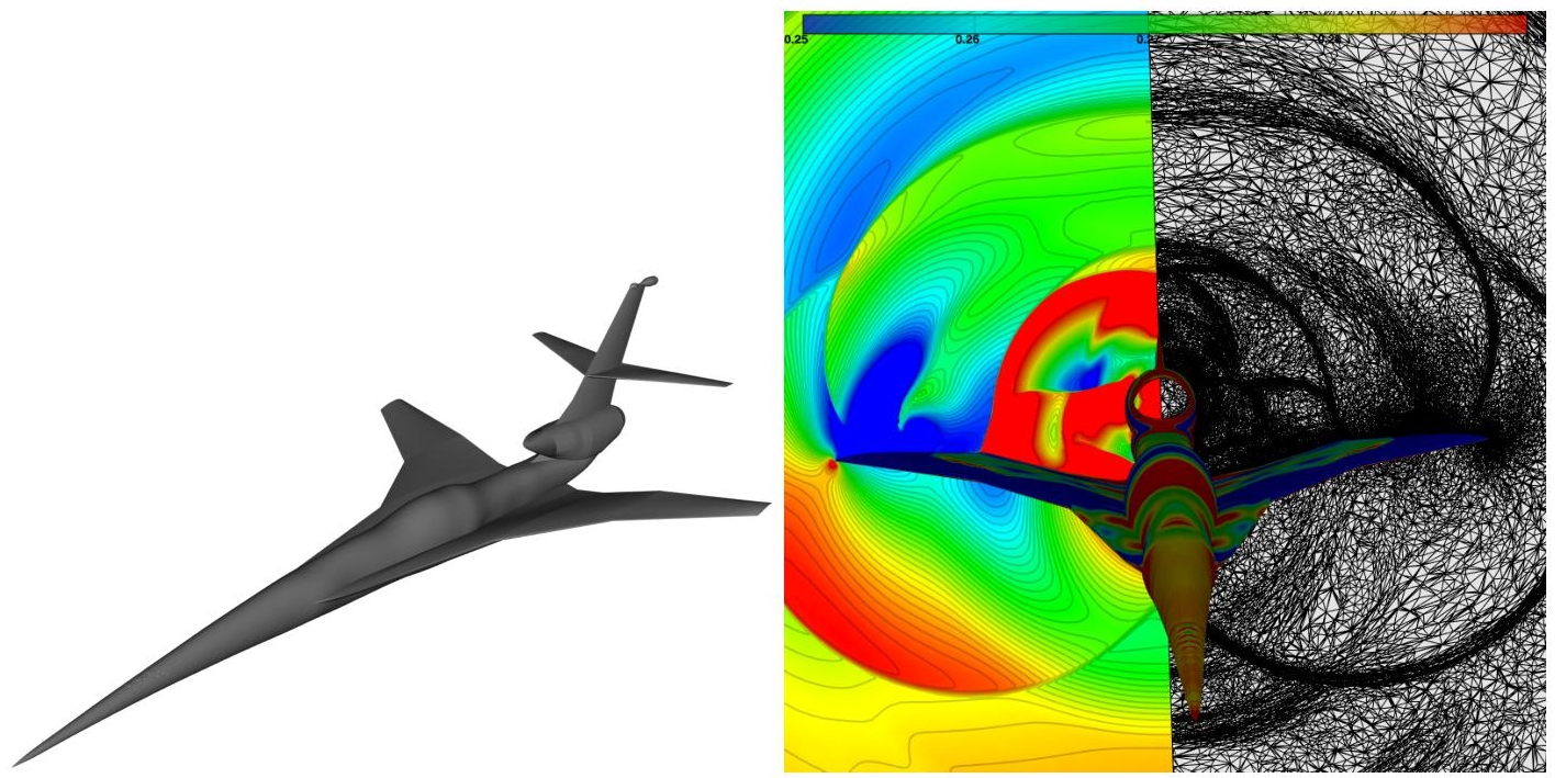
Figure 1.3. Second AIAA Sonic Boom prediction workshop. Left: C25D geometry. Right: Cut plane in the volume behind the aircraft where we can observe in the left part the Mach field and in the right part the 5.9 million vertices adapted mesh obtained with a goal-oriented mesh adaptation on the pressure signature. For a color version of this figure, see www.iste.co.uk/dervieux/meshadaptation2
This nonlinear approach has proven to bring a significant improvement for nonlinear problems, removing the dependency on the choices in the linearization. Such a corrector can be useful in the following processes.
First, a corrector is a good postprocessing for increasing the accuracy of a computation on a given mesh, without changing the mesh and without an important extra computational effort. All the numerical examples have demonstrated that this nonlinear corrector provides an efficient and pertinent correction of the solution and in turn an estimation of the numerical error. Further, the corrected solution remains second-order accurate and, in case of mesh convergence, can be used for a Richardson extrapolation.
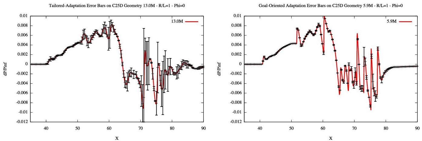
Figure 1.4. Second AIAA Sonic Boom prediction workshop. Pressure difference under the plane (continuous line) for a tailored mesh (left) composed of 13 million vertices and adapted meshes (right) composed of 5.9 million vertices. The estimated error provided by the nonlinear corrector is shown by the vertical error bars. For a color version of this figure, see www.iste.co.uk/dervieux/meshadaptation2
Second, the corrector provides an estimation of the numerical error level that can be used to assess the solution mesh convergence (indicating when to stop the convergence analysis) and to give error bars (quantification of the uncertainties due to the discretization) on the obtained numerical solution. The sonic boom results demonstrate how the corrector can be a very useful complement to mesh adaptation, since it can be checked, very coherently, that the mesh adaptation produce a flow for which the corrector is much smaller than those obtained with insufficient mesh resolution.
Third, the corrector can be used as a representation of the approximation error and replace it in the functional error of a mesh adaption process. This is the principle of the norm-oriented mesh adaptation method that is described in Chapter 6 of this volume.
1.7. Notes
More computations can be found in Frazza et al. (2019).
An important application of the computation of correctors is the derivation of norm-oriented mesh adaptation, as presented in Chapter 6 of this volume.