Tracks

Audio sequencers offer a few types of track. Those most likely to be used in mixing are:

• Audio—in the sequence window, these contain the raw tracks and their audio regions (references to audio files on the hard disk).
• Aux—used mainly for audio grouping and to accommodate effects as part of an aux send setup. In the sequence window, these tracks only display automation data.
• Master—most commonly represents the main stereo bus. In the sequence window, these tracks only display automation data.

Two more types of tracks, though less common, may still be used in mixing:

• MIDI—used to record, edit, and output MIDI information. Sometimes used during mixing to automate external digital units, or store and recall their state and presets. Might also be used as part of drum triggering.
• Instrument—tracks that contain MIDI data, which is converted to audio by a virtual instrument. On the mixer, these look and behave just like audio tracks. Might be used during drum triggering with a sampler as the virtual instrument.

Variations do exist. Cubase, for example, classifies its auxes as FX Channel and Group Channel.

Mixer strips

Figure 11.2 shows the audio mixer strips of various applications, and the collection of different sections and controls each one provides. Audio, aux, and instrument tracks look the same. Master tracks offer fewer facilities, while MIDI tracks are obviously different. We can see that, despite user interface variations, all the applications provide the same core facilities. The mixer strips are very similar to the channel strips found on a console— they have an input, and the signal flows through a specific path and is finally routed to an output. Figure 11.3 shows the simplified signal flow of a typical mixer strip. Since tracks can be either mono or stereo, mixer strips can be either mono or stereo throughout. However, a mixer strip might have mono input that changes to stereo along the signal flow (usually due to the insertion of a mono-to-stereo plugin).

The fader, mute button, and pan control need no introduction. The solo function will be explored shortly, while both automation and meters have dedicated chapters in this book. Other sections are:

• Input selection—determines what signal feeds the mixer strip. The options are either buses or the physical inputs of the audio interface. However, only aux strips truly work that way. Audio strips are always fed from the audio regions in the sequence window. When an audio track is recorded, the input selection determines the source of the recorded material, but the audio is first stored in files, and only then fed to the mixer strip (therefore, any loaded processors are not captured onto disk).
• Output selection—routes the output of the mixer strip to either physical output or a bus. Some applications enable multiple selections so the same track can be routed to any number of destinations. This can be handy in very specific routing schemes (side-chain feed, for example). Commonly, mixer strips are routed to the main physical stereo output.
  

  Figure 11.2 Audio mixer strips of different applications.

• Insert slots—lets us load plugins in series to the signal path, to facilitate the addition of processors. However, insert slots are also used to add effects, as we shall soon see. The order of processing is always top to bottom.
• Send slots—similar to the traditional aux sends, they feed either a pre- or post-fader copy of the signal to a bus, and let us control the send level or cut it altogether. Each send slot can be routed to a different bus, and the selection is made locally per mixer strip (i.e., two mixer strips can have their first slots routed to different buses).

Solos

Audio sequencers normally offer destructive in-place solo. Applications such as Cubase and Pro Tools HD also provide nondestructive solos. While some applications let us solosafe a track, others have a solo mechanism that automatically determines which channels should not be muted when a specific track is soloed. For example, soloing a track in Logic will not mute the bus track it is sent to.

Figure 11.3 A signal flow diagram for a typical software mixer strip. Note that the single line can denote either mono or stereo signal path throughout—depending on the track.

Control grouping

Control grouping was mentioned in Chapter 10 as the basic ability to link a set of motorized faders on an analog desk. Audio sequencers provide much more evolved functionality than that. Each track can be assigned to one or more groups, and a group dialog lets us select the track properties we wish to link. These might include mute, level, pan, send levels, automation-related settings, and so on. Figure 11.4 shows the control grouping facility in Logic.

Figure 11.4 Logic’s control grouping. The various backing-vocal tracks all belong to control group 1—called BV. The linked properties are ticked on the group settings window.

Control grouping, or just grouping as it is often termed, can be very useful with editing. However, when it comes to mixing, there is something of a love-hate relationship. On one hand, it removes the need for us to create an additional channel for an audio group. For example, if we have bass-DI and bass-mic, we often want the level of the two linked, and creating an audio group for just that purpose might be something of a hassle. On the other hand, control grouping does not allow collective processing over the grouped channels. There is very little we can do with control grouping that we cannot do with audio grouping. Perhaps the biggest drawback of control grouping is its actual essence— despite grouping a few tracks, often we may wish to alter some of them individually. Some applications provide more convenient means to momentarily disable a group or a specific control of a grouped track.

Audio grouping

Audio grouping provides the freedom to both individually and collectively process. As opposed to consoles, software mixers do not provide routing matrices. To audio-group tracks, we simply set the output of each included track to a bus, then feed the bus into an auxiliary track. We can process each track individually using its inserts, and process the audio group using the inserts on the aux track. Figure 11.5 illustrates how this is done.

Figure 11.5 Audio grouping on a software mixer (Digital Performer). The outputs of the various drum tracks (OH to Tom 3) are routed to bus 1–2, which is selected as the input of an aux track (Drums); the aux track output is set to the stereo bus. By looking at the insert slots at the top, we can see that each track is processed individually, and there is also collective processing occurring on the drum group.

Sends and effects

As already mentioned, the addition of effects is commonly done using the send facility. Individual tracks are sent to a bus of choice, and, similarly to audio grouping, the bus is fed to an aux track. The effects plugin is loaded as an insert on the aux track, and we must make sure that its output is set to wet signal only. The aux track has its output set to the stereo mix. Figure 11.6 illustrates this.

Other routing

The input/output routing facility can be useful for more than grouping and sends. For example, a compressor loaded on the insert slots is pre-fader, but what if we wish to gain-ride the vocals and only then apply compression? We can route the output of the vocal track to an aux and insert the compressor on that aux. Figure 11.7a shows how this is done in Logic. A small trick provides a better alternative to this situation: we can insert a gain plugin before the compressor and gain-ride the former (Figure 11.7b). However, this might not be the ideal solution if we want to use a control surface to gain-ride the fader. Cubase provides an elegant solution to affairs of this kind—each mixer strip offers both pre- and post-fader inserts.

Naming buses (housekeeping tip)

All audio sequencers let us label the physical inputs, the outputs, and the buses. If we fully mix inside-the-box, we do not use physical inputs and we only use one stereo output, so the naming of these is less critical. But a complex mix might involve many buses, and very easily we can forget the purpose of each bus. Scrolling along the mixer trying to trace the function of the different buses is time-consuming. This time can be saved if we label each bus as soon as it becomes a part of our mix. Figure 11.8 shows the same setup as in Figure 11.6 but with the reverb bus labeled.

Figure 11.6 Sends on a software mixer (Pro Tools). Each vocal track is sent to bus 1–2. The aux track input is set to bus 1–2, and the output to the stereo bus. Also, the plugin wet/dry control is set to fully wet. In this setup, the audio tracks provide the dry signal (since each track has its output set to the stereo bus) and the wet signal is all the aux adds.

Figure 11.7 (a) Setting a track output to a bus and feeding it into an aux track lets us perform gain-riding before compression. The signal will travel through the EQ, the audio track fader (Vox Pre), which we gain-ride, the aux compressor, and the aux fader (Vox). (b) The same task can be achieved if we place a gain plugin before the compressor and automate the gain plugin instead of the fader. The signal will travel through the EQ, the gain plugin, which we automate, the compressor, and the audio track fader.

Figure 11.8 Pro Tools I/O setup (one place where buses can be labeled) and a mixer with a labeled bus.

Integer notation

Digital waveforms are represented by a series of numbers. The sample rate defines the number of samples per second, and each sample holds a number that represents the amplitude of the waveform at a specific fraction of time. The possible values used to represent the amplitude are determined by the number of bits each sample consists of, along with the notation used to represent the numbers. If each sample is noted as a 16-bit integer, the possible values are 0 to 65,535 (negative integer notation is ignored throughout this section for simplicity). The highest amplitude a 16-bit sample can accommodate is represented by the number 65,535, which on a peak meter would light the full scale. Such a full-scale amplitude equals 0 dBFS, which is the highest possible level any digital system can accommodate. Mixing digital signals is done by summing (adding) sample values. Summing two samples with the value of 60,000 should result in 120,000. But since 16 bits cannot hold such a large number, a digital system will trim the result down to 65,535. Such trimming results in clipping distortion—normally, an unwanted addition. The same thing happens when we try to boost a signal beyond the highest possible value. Boosting by approximately 6 dB is done by doubling the sample value. Boosting a value of 40,000 by 6 dB should result in 80,000, but a 16-bit system will trim it down to 65,535.

Floating-point notation

Audio files are most commonly either 16- or 24-bit integer, and a D/A converter expects numbers in such form. However, audio sequencers handle digital audio with a different notation called floating-point, which is slightly more complex than the integer notation. With floating-point, some of the bits (the mantissa) represent a whole number, while other bits (the exponent) dictate how this number is multiplied or divided. It might be easier to understand how the floating-point notation works if we define a simplified system where, in a four-digit number, the three rightmost digits represent a whole number (the mantissa), and the leftmost digit defines how many zeros should be added to the right of the mantissa. For example, with the value of 3256, the whole number is 256 and three zeros are added to its right, resulting in 256,000. On the same basis, the value 0178 is equal to 178 (no added zeros). The most common floating-point notation, which has 24 bits of mantissa and 8 bits of exponent, is able to represent an enormous range of numbers, whether extremely small or extremely large. A 16-bit floating-point system supports much smaller and much larger values than a 16-bit integer system. As opposed to its integer counterpart, on a 16-bit floating-point system 60,000 + 60,000 does result in 120,000.

While the range of numbers supported by modern floating-point systems extends beyond any practical calculations mankind requires, there are some precision limitations attached. In the four-digit simplified system above, we could represent 256,000 and 178, but there is no way to represent the sum of both: 256,178. Floating-point can support very small or large numbers, but no number can extend beyond the precision of the mantissa. A deeper exploration into the floating-point notation reveals that each mantissa always starts with binary 1, so this “implied 1” is omitted and replaced with one more meaningful binary digit. Thus, the precision of the mantissa is always one bit larger than the number of bits it consists of. For instance, a 24-bit mantissa has an effective precision of 25 bits.

The precision of the mantissa defines the dynamic range of a digital system, where each bit contributes around 6 dB (more closely 6.02, or precisely 20log2). Many people wrongly conclude that the famous 32-bit floating-point notation has 193 dB of dynamic range, when in practice the 25-bit mantissa only gives us around 151 dB. Two samples on such a system can represent a very high amplitude or an extremely low amplitude, which can be around 1,638 dB apart. However, when the two samples are mixed, the loud signals “win” the calculation, and any signal 151 dB below it is removed. In our four-digit simplified system, the result of 256,000 + 178 would be 256,000.

What is in it for us?

The internal architecture of audio sequencers is based on the 32- bit floating-point notation (Pro Tools HD also uses fixed-point notation, which is very similar). The audio files that constitute the raw tracks are converted from integers to 32-bit float on-the-fly during playback. The audio data is kept as floating-point throughout the mixer, and is only converted back to integers prior to the D/A conversion or when bouncing to an integer-based audio file (Figure 11.9). From the huge range of values 32-bit float numbers can accommodate, sample values within the application are in the range of –1.0 to 1.0 (the decimal point denotes a float number). This range, which can also be considered as –100 to 100 percent, was selected as it allows the uniform handling of different integer bit depths— a value of 255 in an 8-bit integer file, and a value of 65,535 in a 16-bit file are both full-scale; thus both will be represented by 1.0 (100 percent).

We know already that a 16-bit integer system clips when two full-scale (65,535) samples are summed. Audio sequencers, with their 32-bit float implementation, have no problem summing two sample values of 1.0 (integer full-scale)—software mixers live peacefully with sample values such as 2.0, 4.0, 808.0, and much larger numbers. With such an ability to overshoot the standard value range, we can theoretically sum a million tracks at integer full-scale, or boost signals by around 764 dB, and still not clip on a 32-bit floating-point system. Practically speaking, even the most demanding mix would not cause clipping in the 32-bit floating-point domain.

However, we are all aware that audio sequencers do clip, and that the resultant distortion can be quite obvious and nasty. The reason behind this is that at some point the float data is converted back to integer, and 1.0 is converted back to integer full-scale (65,535 for 16 bits). During this conversion, a value above 1.0 is trimmed back to 1.0, which causes clipping distortion just like when integers are trimmed. The key point to remember here is that trimming—and its subsequent clipping distortion—can only happen during the float-to-integer conversion, nowhere else within the software mixer. This conversion is applied as the mix leaves the master track, therefore only overshooting signals at this stage will cause clipping distortion. While all mixer strips provide a clipping indicator with a threshold set to 1.0, none of these indicators denotes real clipping distortion—apart from the one on the master track.

Figure 11.9 Macro audio flow in an audio sequencer and integer/float conversions.

As unreasonable as this fact might seem, it can be easily demonstrated by a simple experiment that is captured in Figure 11.11. We can set up a session with one audio and one master track, set both faders to unity gain (0 dB), then insert a signal generator on the audio track and configure it to generate a sine wave at 0 dB. If we then bring up the audio fader by, say, 12 dB, both clip indicators will light up (assuming post-fader metering), and clipping distortion will be heard. However, if we then bring down the master fader by 12 dB, the clipping distortion disappears, although the clipping indicator on the audio track is still lit up. By boosting the sine wave by 12 dB, it overshoots and thus the clipping indicator lights up. But, as the master fader attenuates it back to a valid level of 0 dB, it does not overshoot the master track, following which real clipping distortion occurs.

It is worth knowing that clipping-distortion will always occur when a clipping mix is bounced, but not always when it is monitored. This is dangerous since a supposedly clean mix might distort once bounced. Both Pro Tools and Cubase are immune to this risk as the monitored and bounced mixes are identical. However, when a mix clips within Logic or Digital Performer, clipping distortion might not be audible due to headroom provided by certain audio interfaces. Still, the mix will distort once bounced. Monitoring the master track clipping indicator in these applications is vital.

Figure 11.10 This Pro Tools screenshot shows a signal first being boosted by 12 dB by the audio track fader, then attenuated by the same amount using the master fader. Despite the lit clipping indicator on the audio track, this setup will not generate any clipping distortion.

If individual tracks cannot clip, what is the point of having clipping indicators? A few possible issues make it in our interest to keep the audio below the clipping threshold. First, some processors assume that the highest possible sample value is 1.0—a gate, for example, will not act on any signals above this value, which represents the gate’s highest possible threshold (0 dB). Second, the more signals there are crossing the clipping threshold, the more likely we are to cause clipping on the master track. While we will soon see that this issue can be easily resolved, why cure what can be prevented? Last, some plugins—for no apparent reason—trim signals above 1.0, which generates clipping distortion within the software mixer. To conclude, flashing clipping indicators on anything but the master track are unlikely to denote distortion, yet:

Clipping indicators are also integrated into some plugins. It is possible, for example, that a boost on an EQ will cause clipping on the input of a succeeding compressor. It is also possible that the compressor will bring down the level of the clipping signal to below the clipping threshold, and thus the clipping indicator on the mixer strip will not light up. The same rule applies to clipping within the plugin chain—they rarely denote distortion, but it is wise to keep the signals below the clipping threshold.

Bouncing

It is worth explaining what happens when we bounce—whether it be intermediate bounces or the final mix bounce. If we bounce onto a 16-bit file, we lose 9 bits of dynamic range worth 54 dB. These 54 dB are lost forever, even if the bounced file is converted back to float during playback. Moreover, such bit reduction introduces either distortion or dither noise. While not as crucial for final mix bounces, using 16-bit for intermediate bounces simply impairs the audio quality. It would therefore be wise to bounce onto 24-bit files. Another issue is that converting from float to integer (but not the other way around) impairs the audio quality to a marginal extent. Some applications let us bounce onto 32-bit float files, which means that the bounced file is not subject to any degradation. However, this results in bigger files that might not be supported by some audio applications, including a few used by mastering engineers.

Dither

Within an audio system, digital distortion can be the outcome of either processing or bit reduction. Digital processing is done using calculations involving sample values. Since memory variables within our computers have limited precision, sometimes a digital system cannot store the precise result of a specific calculation. For example, a certain fader position might yield a division of a sample value of 1.0 by 3, resulting in infinite 3s to the right of the decimal point. In such cases, the system might round off the result, say to 0.333334. Since the rounded audio is not exactly what it should be, distortion is produced. Essentially, under these circumstances, the system becomes nonlinear just like any analog system. Luckily, the distortion produced by calculations within our audio sequencer is very quiet and in most cases cannot be heard. The problems start when such distortion accumulates (a distortion of distortion of distortion, etc.). Some plugin developers employ double-precision processing. Essentially, calculations within the plugin are done using 64-bit float, rather than 32-bit float. Any generated distortion in such systems is introduced at far lower levels (around –300 dB). But in order to bring the audio back to the standard 32-bit float, which the application uses, the plugin has to perform bit reduction. Unless dither is applied during this bit reduction, a new distortion is produced.

The reason bit reduction produces distortion is that whenever we convert from a higher bit depth to a lower one, the system truncates the least meaningful bits. This introduces errors into the stream of sample values. To give a simplified explanation why: if truncating was to remove all the digits to the right of the decimal point in the sequence 0.1, 0.8, 0.9, 0.7, the result would be a sequence of zeros. In practice, all but the first number in our example are closer to 1 than to 0. Bit reduction using rounding would not help either, since this would produce rounding errors—a distortion sequence of 0.1, 0.2, 0.1, 0.3.

Dither is low-level random noise. It is not a simple noise, but one that is generated using probability theories. Dither makes any rounding or truncating errors completely random. By definition, distortion is correlated to the signal; by randomizing the errors, we decorrelate them from the signal and thus eliminate the distortion. This makes the system linear, but not without the penalty of added noise. Nonetheless, this noise is very low in level—unless accumulating.

But the true power of dither is yet to be revealed: dither lets us keep the information stored in the truncated bits. The random noise stirs the very-low-level details into the bits that are not truncated, and thus the information is still audible even after bit reduction. The full explanation of how exactly this happens is down to the little-known fact that digital systems have unlimited dynamic range, but they do have a defined noise floor. This noise floor is determined, among other things, by the bit depth. In practice, a 16-bit system provides unlimited dynamic range, but it has its noise floor at around –96 dB. Human beings can discern information below that noise floor, but only to a point. If dither is not applied, the information in the truncated bits is lost, and distortion is produced. With dither, there is no distortion and the low-level details are maintained. However, at some point, they will be masked in our perception by the noise.

Theoretically, any processing done within a digital system can result in digital distortion. This includes compressors, equalizers, reverbs, and even faders and pan pots. Due to its huge range of numbers, any floating-point system is far less prone to digital distortion compared with an integer system. Within an audio sequencer, most of this distortion is produced around the level of –140 dB, and for the most part would be inaudible. Manufacturers of large-format digital consoles apply dither frequently along the signal path. This is something audio sequencers do not do, but many plugins do (as part of double-precision processing). Dither has to be applied in the appropriate time and place. There is no point in us randomly adding dither, since doing so would not rectify the distortion—it would just add noise on top of it. The only instance where we should dither is as part of bit reduction. Such bit reduction takes place every time we bounce onto 16-bit files. We have just seen that bit reduction also causes distortion when bouncing onto 24-bit files, so there is a rationale for dithering even when bouncing onto such files. Only if we bounce onto 32-bit float files (Cubase, for example, enables this) do we not need to dither. The rule of dither is therefore very simple:

The generation of dither noise is not a simple affair. Different manufacturers have developed different algorithms; most of them involve a method called noise-shaping that lets us minimize the perceived noise level. Since our ears are less sensitive to noise at specific frequencies, shifting some of the dither energy to those frequencies makes the noise less apparent. There are different types of noise-shaping, and the choice is usually done by experimentation.

Most audio sequencers ship with dither capabilities. It might be an individual plugin, a global option, or part of the bounce dialog. In addition, more than a few plugins, notably limiters and loudness-maximizers, provide dither as well. Essentially, what the dither process does is add dither noise, then remove any information below the destination bit depth. Figure 11.11 shows a dither plugin. The plugin is loaded on the master track in Pro Tools to establish itself as the very last process (even after the master fader). We can see the typical dither parameters: destination bit depth and noise-shaping type. In this case, the plugin is preparing for a bounce onto a 16-bit file.

Normalization

Figure 11.12 shows two audio regions. It is worth mentioning how the scale in Pro Tools works (or any other audio sequencer, for that matter). The middle mark is complete silence, otherwise roughly –151 dB; the top mark is 0 dB. Then every halving of the scale is worth –6 dB. The majority of the display shows the high-level part of the signal—there is as much space to show level variations between –12 and –18 dB as there is from –18 to –151 dB.

Figure 11.11 Pro Tools’ POWr Dither plugin.

Figure 11.12 Waveform display scales. The left and right regions are identical, except that the right region is 18 dB quieter than the left one. The scales in editor windows are divided so that each halving results in –6 dB of level. The majority of what we see is the loud part of the waveform.

Consequently, it might seem that the right region is substantially lower in level than the left region, but in fact the left region is only 18 dB lower in level.

We often want our signals to be at optimum levels. An offline process called normalization lets us do this—it boosts the signal level to maximum without causing any clipping. For example, if the highest peak is at –18 dB, the signal will be boosted by 18 dB. As an offline process, normalization creates a new file that contains the maximized audio. Normalization, however, has its shortcomings. During the process, rounding errors occur, resulting in the same distortion just discussed. This is especially an issue when 16-bit files are involved.

Normally, loud recordings are not placed next to quiet recordings as in Figure 11.12— we often simply have a whole track low in level. A more quality-aware approach to normalization involves boosting the audio in realtime within the 32-bit float domain. This can be easily done by loading a gain plugin on the first insert slot of the low-level track. This is very similar to the analog practice of raising the gain early in the signal-flow path when the signal on tape was recorded too low.

The master fader

Due to the nature of float systems, the master fader in audio sequencers is, in essence, a scaling fader. It is so-called since all it does is scale the mix output into a desired range of values. If the mix clips on the master track, the master fader can scale it down to an appropriate level. It is worth remembering that a master track might clip even if none of the individual channels overshoots the clipping threshold. In these situations, there is no need to bring down all of the channel faders—simply use the master fader. In the opposite situation, where the mix level is too low, the master fader should be used to scale it up.

This is also worth keeping in mind when bouncing. The master fader (or more wisely a gain plugin on the master track) should be used to set the bounced levels to optimum. Determining the optimum level is easy if we have a numeral peak display—we have to reset the master track’s peak display and play the bounce range once. The new reading on the peak display will be equal to the amount of boost or attenuation required to bring the signal to 0 dB (or to the safety –3 dB) (Figure 11.13).

Figure 11.13 The master track in Cubase after the bounced range has been played. The top value shows the peak measurement (–11.9 dB) and tells us that the master fader can be raised by nearly 11.9 dB before clipping will occur.

The master track in Pro Tools is worth mentioning. As opposed to all the other track types, a master track in Pro Tools has its inserts post-fader. This is in order to enable dithering at the very last stage in the digital signal chain. The consequence of this is that any dynamic processing applied on the master track, such as limiting, will be affected by the master fader. If we automate, or fade out the master fader, the amount of limiting and its sonic effect will vary (Figure 11.14a). Although seldom desired, such an effect can be heard on a few commercial mixes. To fix this issue, individual tracks are routed to a bus that feeds an auxiliary, and the limiting is applied on the auxiliary. The dithering is applied on the master track (Figure 11.14b). Here again, having both pre- and post-inserts per mixer strip, like in Cubase, would be very handy.

The playback buffer

Audio sequencers handle audio in iterations. During each iteration, the application reads samples from the various audio files, processes the audio using the mixer facilities and plugins, sums all the different tracks, and delivers the mix to the audio interface for playback. Each iteration involves a multitude of buffers; each represents a mono track or a mono bus. The playback buffer size determines how many audio samples each of these buffers holds. For example, if the playback buffer size is 480 samples, during each iteration 480 samples from each file are loaded into the track buffers; each plugin only processes 480 samples, and the different tracks are summed into the mix-bus buffer, which also consists of 480 samples. Once the mix buffer has been calculated, it is sent to the audio interface. If the buffer size is 480 samples and the playback sample rate is set to 48,000, it will take the audio interface exactly 10 ms to play each mix buffer. While the audio interface is playing the buffer, another iteration is already taking place. Each iteration must be completed, and a new mix-buffer delivered to the audio interface, before the previous buffer finishes playing (less than 10 ms in our case). If an iteration takes longer than that, the audio interface will have nothing to play, the continuous playback will stop, and a message might pop with a CPU overload warning. A computer must be powerful enough to process audio in real time faster than it takes to play it back.

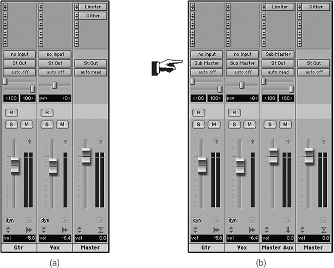
Figure 11.14 (a) Since the limiter on the master track is post-fader, any fader movements will result in varying limiting effect. (b) The individual audio tracks are first routed to an auxiliary, where limiting is applied, and only then sent to the main output, where dithering takes place post-fader. Note that in this setting both the aux and the master faders succeed the limiter, so both can be automated. Automating the aux is preferred, so the master fader remains as an automation-independent scaling control.

The playback buffer size determines the monitoring latency of input signals, and the smaller the buffer size, the lower the input latency. This is important during recording, but less so during mixdown, where input signals are rarely involved. Smaller settings, however, also mean more iterations—each with its own processing overhead—so fewer plugins can be included in the mix. With a very small buffer size (say, 32 samples), some applications might become unpredictable, start producing clicks, or skip playback. However, depending on the application, large buffer size can affect the accuracy of some mix aspects, such as automation. When choosing the buffer size, it should be large enough to allow a sufficient number of plugins and predictable performance; anything larger than that might not be beneficial. A sensible buffer size to start experimenting with is 1,024 samples.

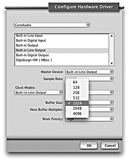
Figure 11.15 Digital Performer’s configuration window where the playback buffer size is set.

Plugin delay compensation

We have just seen that plugins process a set number of samples per iteration. Ideally, a plugin should be given an audio buffer, process it, and output the processed buffer straight away. However, some plugins can only output the processed buffer a while after, which means their output is delayed. There are two reasons for such plugin delay. The first involves plugins that run on a DSP expansion such as the UAD card. Plugins of this kind send the audio to the dedicated hardware, which returns the audio to the plugin after it has been processed. It takes time to send, process, and return the audio; therefore, delay is introduced. The second reason involves algorithms that require more samples than those provided by each playback buffer. For example, a linear-phase EQ might require around 12,000 samples in order to apply its algorithm, which falls short of the common 1,024 samples the plugin gets per iteration. To overcome this, the plugin accumulates incoming buffers until these constitute a sufficient number of samples. Only then, after some time has passed, does the plugin start processing the audio and output it back to the application.

Plugin delay, in its least harmful form, causes timing mismatches between various instruments, as if the performers are out of time with one another. A mix like that, especially one with subtle timing differences, can feel very wrong, although it can be hard to pinpoint timing as the cause. In its most harmful form, plugin delay causes comb filtering, tonal deficiencies, and timbre coloration. For example, if plugin delay is introduced on a kick track, it might cause comb filtering when mixed with the overheads.

Luckily, all audio sequencers provide automatic plugin delay compensation. In simple terms, this is achieved by making sure that all audio buffers are delayed by the same number of samples.