
4
Particular Applications
Among the distinctive and illustrative applications of the fundamental principle, the Earth’s motion is one particularly unique example. Indeed, it is highly complex, but simplified approaches can be made for the purposes of demonstration. One of the important factors of this complexity is the model which should be used to describe the body in motion since its inertial characteristics play a fundamental role in the expression of the equation. So, in the context of a simplified approach, we can consider that the Earth is a simple sphere, rotating around its polar axes; or an ellipsoid rotating around the same axis. Different approaches will be explored in the following section.
Foucault’s pendulum is another interesting case. This section is mostly drawn from the article published by Michel Cazin in the magazine Sciences of July 2000, pp. 44–59; in no way does the present chapter claim to present that particular work which is very in-depth and largely surpasses the scope of this title. We will simply lead the developments towards the movement equations and will present the conclusions surrounding motion reached by the author.
4.1. Simulation of the motion of Earth
4.1.1. Application of the fundamental principle
The Earth is not subject to any linkage; its motion is mainly due to the various forces of attraction that the bodies of the solar system apply onto it. Therefore, in the context of the application of the fundamental principle, it is treated as a free solid (S) in motion in the Galilean frame ❬g❭. The fundamental principle applied to its motion is stated
In the development that we will perform, the torsor { Δ } is a vector torsor with a null moment at the center of inertia G of the solid, thus the two following vectorial equations.

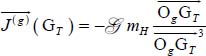
Upon first approximation, we also consider that the torsor of gravitational forces exerted by the Sun upon the Earth is a vector torsor with a null moment at the center of inertia GT of the Earth and the resultant

GH and GT are the centers of inertia of the Sun (H) and of the Earth (T), mH and mT are their respective masses, ![]() is the universal gravitational constant.
is the universal gravitational constant.
The main characteristic values of the problem are

In the following developments, we focus first of all on the motion of a solid (S) with a center of inertia G to which we apply the hypotheses we wish to explore. Next, if necessary, we explore their application to the case of Earth with its own set of data.
The two vector consequences of the fundamental principle, the equality between resultants known as the theorem of dynamic sum, and the equality between the moments at a same point, known as the theorem of dynamic moment in G, express two different aspects of the problem: the first focuses more specifically on the motion of the center of inertia of the solid and its trajectory, while the second focuses on the behavior of the solid around its center of inertia, during its progression along its trajectory.
4.1.2. Theorem of dynamic moment at G
This theorem corresponds to the vector equality of moments stemming from the torsor relation of the fundamental principle; it is therefore expressed by
with
To precise the way in which we will process the following question, we consider that:
- – the principal inertia basis in G of the solid (S) is
 ;
; - – the inertia matrix of the solid (S) in that basis is

- – the rotation rate of the solid (S) in relation to ❬g❭ is
and its derivative relative to time
The dynamic moment at G then has the following expression

If we consider the expression of the kinetic moment
considering that

we easily verify that ![]() .
.
We therefore deduce that the kinetic moment at G of the solid (S) throughout its motion in the Galilean frame ❬g❭ is independent of time
The theorem of dynamic moment therefore results in three scalar consequences

When this solid is Earth, it is a matter of examining the result of these differential equations according to the inertial model we choose to represent it with.
4.1.2.1. First case A = B = C
In this case, we have
The rotation rate ![]() is then independent of time in the motion of the solid (S) in ❬g❭; as
is then independent of time in the motion of the solid (S) in ❬g❭; as
the rotation rate vector ![]() is also independent of time in ❬S❭. According to the three scalar consequences of the theorem of dynamic moment
is also independent of time in ❬S❭. According to the three scalar consequences of the theorem of dynamic moment

In the selected case, Earth is considered as a non-deformable homogeneous sphere with concentric layers. The unit vector ![]() is driven on the axis of the poles and oriented South to North. The Earth then revolves with a constant angular velocity
is driven on the axis of the poles and oriented South to North. The Earth then revolves with a constant angular velocity
We therefore have: ![]() .
.
4.1.2.2. Second case A = B ≠ C
The three scalar consequences of the theorem of dynamic moment at G are

4.1.2.2.1. Determining the rotation rate
The third equation of section 4.1.2.2 leads to the result
which shows that the component on ![]() of the rotation rate is independent of time.
of the rotation rate is independent of time.
Stating ![]() , the first two relations become
, the first two relations become
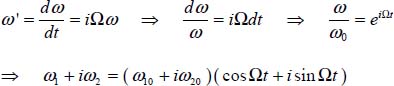
Adding the two above relations after multiplying the second by the complex number r, we obtain
and setting ω = ω1 + iω2, we have
The rotation rate of the solid (S) in ❬g❭ therefore has the components in the base ![]()


As ![]() , in the frame
, in the frame ![]() , the extremity of the rotation rate vector
, the extremity of the rotation rate vector ![]() , of origin G, draws a circle with a radius of
, of origin G, draws a circle with a radius of ![]() , (0, 0, ω30) as its center, and the axis
, (0, 0, ω30) as its center, and the axis ![]() , with a constant angular velocity Ω.
, with a constant angular velocity Ω.
4.1.2.2.2. Eulerian configuration of the motion
Let us now locate the basis ![]() in relation to the basis
in relation to the basis ![]() via the Euler angles ψ,θ,ϕ according to the following diagram
via the Euler angles ψ,θ,ϕ according to the following diagram


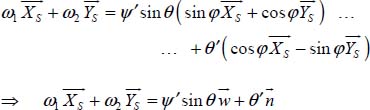
Accounting for the previously calculated components of ![]() , we obtain
, we obtain

Generally, we can’t only determine the Euler angles from these relations. This determination is only possible if we introduce new conditions upon the motion of the solid (S). We will therefore emit the hypothesis that the vector ![]() is the unit vector of the kinetic moment, so
is the unit vector of the kinetic moment, so
As with
the expression of the kinetic moment is
As the three vectors ![]() and
and ![]() are all three orthogonal to
are all three orthogonal to ![]() , the component of the kinetic moment on this last vector gives us
, the component of the kinetic moment on this last vector gives us
The nutation angle is subsequently independent of time.
Also, we have ![]() ; we obtain for the expression of the kinetic moment
; we obtain for the expression of the kinetic moment
and in identifying the components, the two relations
In the case where θ0 is non-null, we get
To recap, in the case where A = B ≠ C, the motion of (s) in relation to ❬g❭ occurs with a constant nutation θ0, a constant precession velocity ![]() and a constant spin velocity
and a constant spin velocity ![]() .
.
4.1.2.2.3. Properties of the rotation rate
In the studied case, the rotation rate has the following expression
and its derivative in relation to time in ❬g❭
keeps a constant modulus.
The unit vectors ![]() and
and ![]() keep a constant angle throughout the motion of the solid; the same goes for the components of
keep a constant angle throughout the motion of the solid; the same goes for the components of ![]() on these two axes.
on these two axes.
As ![]() makes a constant angle with
makes a constant angle with ![]() , its support draws in the frame ❬g❭ an axoid surface (A(g)) which is shaped like a cone. Similarly,
, its support draws in the frame ❬g❭ an axoid surface (A(g)) which is shaped like a cone. Similarly, ![]() forms a constant angle with
forms a constant angle with ![]() and its support draws in the frame
and its support draws in the frame ![]() an axoid surface (A(s)) which is also shaped like a cone.
an axoid surface (A(s)) which is also shaped like a cone.
The motion of (A(s)) in relation to ❬g❭ is obtained by a non-sliding roll of the cone (A(s)) over the cone (A(g)). If ![]() and
and ![]() are both positive, the two cones are exterior; if
are both positive, the two cones are exterior; if ![]() is positive and
is positive and ![]() negative, the cone (A(g)) is inside the cone (A(s)).
negative, the cone (A(g)) is inside the cone (A(s)).

In the second case above, the Earth is represented by a revolving ellipsoid flattened at the poles. The unit vector ![]() is carried by the axis of the poles,
is carried by the axis of the poles, ![]() is located along the Greenwich Meridian plane. C is the moment of inertia relating to the South towards North axis and A the one relating to a diameter of the equatorial plane.
is located along the Greenwich Meridian plane. C is the moment of inertia relating to the South towards North axis and A the one relating to a diameter of the equatorial plane.

For Earth, we are in the second case mentioned, with ![]() and
and ![]() . ω10 and ω20 are small compared to ω30, θ0 and
. ω10 and ω20 are small compared to ω30, θ0 and ![]() are small.
are small.
4.1.3. Theorem of dynamic resultant
This theorem corresponds to the vector equality of the resultants deduced from the torsor relation of the fundamental principle; it is thus expressed as
The study of the motion of the center of inertia G of the solid depends on the hypotheses made about the term ![]() . Two cases are considered here; the first one is that of a constant vector in ❬g❭, the second is that of a vector collinear to
. Two cases are considered here; the first one is that of a constant vector in ❬g❭, the second is that of a vector collinear to ![]() .
.
4.1.3.1. First case
In the first case where ![]() is a constant vector in ❬g❭, the theorem of dynamic resultant has the following consequences
is a constant vector in ❬g❭, the theorem of dynamic resultant has the following consequences

The vectors ![]() and
and ![]() are all three independent of time in ❬g❭:
are all three independent of time in ❬g❭:
- – if
 , the trajectory of G in ❬g❭ is a straight line,
 - – if
 , the trajectory of G in ❬g❭ is a parabola.
4.1.3.2. Second case
In the second case where ![]() is a vector collinear to
is a vector collinear to ![]() , the theorem of dynamic resultant is written
, the theorem of dynamic resultant is written

4.1.3.2.1. Motion constants

where ![]() is a vector independent of time in ❬g❭.
is a vector independent of time in ❬g❭.
Subsequently, ![]() is orthogonal to a constant vector in ❬g❭; the trajectory of G in ❬g❭ is a plane curve.
is orthogonal to a constant vector in ❬g❭; the trajectory of G in ❬g❭ is a plane curve.
In the case of Earth, we ignore the gravitational actions that would not be due to the Sun, that is any effects coming from the Moon and other planets of the solar system. We can then write

The motion of the center of inertia of the Earth is given by the theorem of dynamic resultant, that is
By setting

the application of the theorem of dynamic sum gives
which verifies ![]() .
.
We thus find once again
![]() , with vector
, with vector ![]() independent of time in ❬g❭
independent of time in ❬g❭
![]() being orthogonal to a constant vector in ❬g❭, the trajectory of the point G in the frame ❬g❭ is a plane curve located in the plane
being orthogonal to a constant vector in ❬g❭, the trajectory of the point G in the frame ❬g❭ is a plane curve located in the plane ![]() called the ecliptic plane.
called the ecliptic plane.
We set  and consider the basis
 ![]() such that
such that ![]() belongs to the ecliptic plane
belongs to the ecliptic plane ![]() . We also set
. We also set


The theorem of the dynamic resultant is then written
and has the following scalar consequences

The term ![]() , called orthoradial acceleration, is null. Subsequently r2αʹ is independent of time and equal to the constant of areas C.
, called orthoradial acceleration, is null. Subsequently r2αʹ is independent of time and equal to the constant of areas C.
The motion of the center of inertia in the Galilean frame ❬g❭ is therefore governed by these two equations
As

the elementary area of the curvilinear section swept by the vector radius is
and the quantity ![]() , called the areal velocity, is constant.
, called the areal velocity, is constant.
4.1.3.2.2. Equation of the trajectory of the Earth’s center of inertia
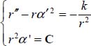
The equation for the trajectory is obtained by eliminating the time parameter between two equations

The two equations that give us the trajectory then become
a quadratic linssear differential equation with constant coefficients that allows for a solution of the following form
The trajectory in ❬g❭ of the center of inertia GT of Earth is conic and its equation can be put into a polar form
where e is the eccentricity, the value of which defines the nature of the conic (circle, ellipse, hyperbola, parabola).
As
through identification, we obtain

4.1.3.2.3. Trajectory analysis
We also consider, to continue the simulation, that the distance of the Earth’s center of inertia at the origin of the Galilean frame is constant, meaning thassst r = r0; the two equations that govern the motion of GT become

But ![]() .
.
At initial time t0, ![]() with
with ![]() .
.
The initial velocity of GT is thus orthogonal to the vector radius carried by ![]() at that time and has the following expression
at that time and has the following expression
In this diagram, the Earth’s center of inertia performs, at a constant velocity in the ecliptic plane, a circular trajectory of radius r0.

4.2. Foucault’s pendulum
4.2.1. Observation of the phenomenon
The works of Foucault, in particular the ones with regards to gyroscopes and pendulum motion, highlighted the importance of the choice of the frame. They demonstrated that, by isolating a system from its immediate environment and, in particular, by separating it from any actions that the latter may have been exerting over it, the observed motion of the gyroscope or the pendulum could not be explained in a frame tied to the observation point.
Thus, for the pendulum, only a description of its motion taking into account that of the Earth explains the locally observed rotation of its oscillation plane.
The pendulum was imagined by Foucault and his demonstration at the Panthéon in 1857 consisted of a heavy sphere hung by a 67m long silver wire and tied in such a way that its bond point caused minimal disturbance to its pendular oscillation. Lastly, the weight of the sphere minimized the deformation stress of the suspension wire which was selected so that these stresses could already be very weak. So the pendulum was isolated from the area where its motion was apparently occurring.

The pendulum was launched into oscillation in a vertical plane graduated at time t0 and, throughout its pendulum motion, we observed the behavior of its oscillation plane as it performed a rotation motion around its vertical axis.
This observation can only be explained if the motion of the pendulum is occurring in a frame that is not the local frame its observer is in, and in relation to which the pendulum is rotating. The only rotation that the local frame is subject to is the Earth’s, to which it is strongly attached; the observation indicates that the motion of the pendulum occurs in a frame of which the orientation of the axes is independent of the local rotation motion, that would for example be collinear to the fixed axes of the Solar reference frame. This explanation could be corroborated by an adequate interpretation of the measurement of the angle of rotation of the pendulum’s oscillation plane during the time interval [t0, t1].
4.2.2. Analyzing the phenomenon
4.2.2.1. Schematization of Earth’s motion
The point of application of the pendulum being fixed in relation to Earth, it is therefore a good idea to begin by expressing its dynamics under a usable form for the rest of the development.
Consider a body (2) to which is joined the frame ![]() mobile in relation to a reference frame
mobile in relation to a reference frame ![]() . We already know the trajectory Γg(O2) and the way the point moves along it, that is its velocity
. We already know the trajectory Γg(O2) and the way the point moves along it, that is its velocity ![]() and acceleration
and acceleration ![]() . We also emit the hypothesis that the axis
. We also emit the hypothesis that the axis ![]() maintains a fixed direction in ❬g❭.
maintains a fixed direction in ❬g❭.
We consider the trace of the frame ![]() on the plane
on the plane ![]() , a line the orientation of which is given by the vector
, a line the orientation of which is given by the vector ![]() , with α invariable.
, with α invariable.

The angle β such that
is also invariable. To better describe and study the motion of the body (2), we use another reference basis ![]() to create the schematization of this motion by setting
to create the schematization of this motion by setting

This new basis (1) is tied to the basis (g) in such a way that the planes ![]() and
and ![]() are merged. Their relative situation is defined by the angle ε such that
are merged. Their relative situation is defined by the angle ε such that


Figure 4.9. Situation of the body in the new reference frame
In this new reference frame, the rotation rate of the body is
thus the derivatives relative to time of the vectors of the basis (2)

Consider now the motion of a point fixed to body (2),

The last term of the above expression is expressed

where I is the orthogonal projection of M on the axis ![]()

We obtain the term for the drive acceleration
in the case where the point M is moving in the frame ❬2❭. According to the law of composition of accelerations, we would obtain

We now apply this result to the case where the origin point of the frame ❬1❭ is the center of inertia H of the sun and where the axes ![]() ,
, ![]() and
and ![]() are pointed towards fixed stars, where the origin point of the frame ❬2❭ is the center of inertia G of the Earth and
are pointed towards fixed stars, where the origin point of the frame ❬2❭ is the center of inertia G of the Earth and ![]() the South to North axis, which is the polar axis oriented towards a known fixed star.
the South to North axis, which is the polar axis oriented towards a known fixed star.
To simplify, we state that:
- – the Earth’s center of inertia G moves, in the ecliptic plane, on a circle of center HSS, with a radius of 150.106 km, at a constant angular velocity of 2.10-7 rad.s-1;
- – G is subject to a normal constant acceleration of 6.10-4 g, where the gravitational acceleration is g = 9.80665 m.s-2;
- – the Earth is driven with an invariable rotation rate εʹ = 7.3.10-5 rad.s-t (2π rad/day), around the line of the poles SN of unit vector
 , tilted with an angle β neighboring 67° in relation to the ecliptic plane.
The formula of the composition of accelerations is then written, at any point M moving in relation to Earth
4.2.2.2. Study of the motion of the pendulum
This study assumes that the attachment point O2 of the pendulum is fixed in relation to the Earth. This pendulum is essentially composed of a material point M, of mass m. The local frame ![]() , fixed in relation to the Earth, is defined as follows:
, fixed in relation to the Earth, is defined as follows:
- –
 is oriented towards the South;
 - –
 towards the East;
 - –
 towards the zenith (point where the ascending vertical line of the place meets the celestial sphere) of the experiment place.

The reference frame ![]() is Galilean.
is Galilean.
As the solid here is a material point, the fundamental principle of dynamics amounts to the equality of the resultants, that is
where ![]() is the resultant of the outside forces (reaction of the suspension wire marked
is the resultant of the outside forces (reaction of the suspension wire marked ![]() , gravitational attraction of the Earth
, gravitational attraction of the Earth ![]() ) to which is subject the solid assimilated to a material point M.
) to which is subject the solid assimilated to a material point M.
According to the composition of accelerations of a moving point M in relation to Earth
the fundamental principle of dynamics is written
The term “![]() ” being considered negligible1 before “g”, thus the resulting movement equation
” being considered negligible1 before “g”, thus the resulting movement equation
Let us locate the point M via its coordinates in the basis (2)
and, taking into account the fact the wire is non-extensible or deformable, meaning that the three coosssrdinates above are tied by the following relation
where h is constant.
We also state εʹ = Ω = 73.10-6 rad.s-1.
The expression of the fundamental principle then becomes

or

As the vector ![]() is oriented from M towards O2 and the attachment of the wire to the sphere of the pendulum and its coupling at O2 only create an axial traction stress, we can state
is oriented from M towards O2 and the attachment of the wire to the sphere of the pendulum and its coupling at O2 only create an axial traction stress, we can state
where K has the dimension of an acceleration.
We deduce from this the three differential movement equations of the pendulum

For the experiments led by the author, the quantities ![]() and
and ![]() (experimentally < 0.04) were small in relation to the unit, and subsequently
(experimentally < 0.04) were small in relation to the unit, and subsequently
Moreover ![]() is small in relation to xʹ and yʹ.
is small in relation to xʹ and yʹ.
These considerations led Michel Cazin:
- – to neglect the term 2Ωzʹ cos λ before 2Ωxʹ sin λ in the second movement equation above;
- – to write K = g as z" < 1,6.10-3 g and 2Ωyʹ cos λ < 1,2.10-5 g in the third equation,
Hence the two following equations express a coupling between the two components x and y, which are the coordinates of the point P, projection of M on the plane ![]()

If we consider the affix a = x + iy of the point P, via the linear combination of these two equations (1) + i(2), we obtain
If we research a solution of the form
we obtain the relation

which is verified ∀ρ and ∀s with finite values. Subsequently
And in setting
the second degree equation admits the two roots
hence the general solution of the differential equation in a
We will not go into the detail of a complex demonstration as it is not the subject of this present work concerning Foucault’s pendulum, instead we will simply offer the conclusions. However, this type of application shows an entire field of exploration enabled by the movement equations.
The oscillation plane of the pendulum rotates around the axis ![]() of the experiment place with the angular velocity –Ω sin λ. In Paris, this angular velocity is of 5,5.10–5 rad.s-1 in the rotating direction of diurnal motion (that of the Sun for the Northern hemisphere), that is, 11° per hour. At each oscillation of a duration of 8s, the oscillation plane makes 1/40° of a turn2.
of the experiment place with the angular velocity –Ω sin λ. In Paris, this angular velocity is of 5,5.10–5 rad.s-1 in the rotating direction of diurnal motion (that of the Sun for the Northern hemisphere), that is, 11° per hour. At each oscillation of a duration of 8s, the oscillation plane makes 1/40° of a turn2.
Upon first approximation, the motion of the point P in the plane ![]() can be represented by a hypocycloid which is the plane curve obtained as the trajectory of a fixed point on a circle rolling on another wider circle – without slipping – inside the latter, as shown in the following diagram.
can be represented by a hypocycloid which is the plane curve obtained as the trajectory of a fixed point on a circle rolling on another wider circle – without slipping – inside the latter, as shown in the following diagram.

Foucault’s pendulum experiment also points out the essential evidence of the Coriolis acceleration, since with the simplifying hypotheses that the configuration of its motion allows, this term holds a primordial place in the equations that govern this motion.