
We evaluate the performance of EGOR through extensive Monte-Carlo simulations. We compare EGOR with geographic routing, which only has one forwarding candidate that achieves the maximum EPA, and opportunistic routing, which involves all the available next-hop nodes as forwarding candidates. When the packet becomes stuck, all the three protocols just drop the packet. Various situations are simulated by varying node densities, transmission-to-reception energy ratios and retransmission limits.
3.4.1 Simulation Setup
Channel Model: To simulate a realistic channel model for lossy WSNs, we use the log-normal shadowing path loss model derived in (Zuniga and Krishnamachari 2004):
3.8 ![]()
where d is the transmitter–receiver distance, γ(d) is the signal-to-noise ratio (SNR), ρ is the encoding ratio and Lf is the frame length in bytes. This model considers several environmental and radio parameters,3 such as the path-loss exponent (α) and log-normal shadowing variance (σ) of the environment, and the modulation and encoding schemes of the radio. This particular equation resembles a MICA2 mote see the MICA2 datasheet at www.eol.ucar.edu/rtf/facilities/isa/internal/CrossBow/DataSheets/mica2.pdf, which has data rate of 19.2 kbps, and the noise bandwidth 30 kHz. Non-coherent FSK and Manchester are used as the modulation and encoding schemes (ρ = 2), respectively. The environmental parameters are set to α = 3.5 and σ = 4.
Energy Model: The energy consumption is obtained by multiplying the power consumption and the packet transmission time. The transmission power consumption Ptx is the summation of the power of power amplifier (PPA) and electronic (Pelec), and Prx is equal to Pelec. We assume that PPA is proportional to the transmit power Ptrans. Then Ptx is
3.9 ![]()
where η is the PA power efficiency, which is set to be 0.3 in our simulation.
Evaluation Metrics: We define the following metrics to evaluate the performance of the three protocols.
- Packet Delivery Ratio (PDR): percentage of packets sent by the source that actually reach the sink. This is a measure for reliability.
- Energy efficiency η(S, D): this metric is measured in bit-meters per joule (bmpJ). It is calculated as in Equation (3.10),
where Nr denotes the number of packets received at the destination, Lpkt is the packet length in bits, and Etotal is the (transmission and reception) energy consumed by all the nodes involved in the routing procedure excluding the sink. We account for the distance factor, because the energy efficiency is indeed relevant to the distance between the communication pair due to the lossy property of multihop wireless links in WSNs.
- Hop count: it is measured as the number of hops a successfully delivered packet travels from source to destination.
The simulated sensor network has stationary nodes uniformly distributed in a 60 × 60 m2 square region, with nodes having identical fixed transmission power of 0 dbm. The frame length is fixed on 50 bytes with preamble of 20 bytes. The source and the sink node are fixed at two corners across the diagonal of the square area. All simulations are run for 5000 iterations. For each iteration, node locations are randomly reassigned and PRRs between nodes are recalculated.
3.4.2 Simulation Results and Analysis
3.4.2.1 Impact of Node Density
We use different node numbers (100, 144, 196, 225) to achieve various node densities corresponding to the average number of neighbors per node of 9.5, 14, 20, 23 respectively. The reception power consumption is fixed on 2 MW, so the reception to transmission energy ratio is ![]() . No retransmission is allowed.
. No retransmission is allowed.
Figure 3.3 shows that EGOR achieves better energy efficiency than the other two routing protocols. This result can be explained as follows: for every forwarding decision, EGOR chooses the forwarding set that maximizes the EPA per unit energy consumption. This local optimal behavior can achieve a good global performance under a uniformly randomly distributed node deployment, where any intermediate-hop forwarding can be viewed as a similar new first-hop packet forwarding. Statistically, every hop may make similar progress in such a homogeneous environment. The overall energy cost for successfully delivering one packet from source S to destination D can be approximated by ![]() , so when we maximize the numerator, the total energy consumption is minimized. Opportunistic routing involving all the available next-hop nodes in the routing has the worst performance, since it has the lowest EPA/Local energy cost ratio.
, so when we maximize the numerator, the total energy consumption is minimized. Opportunistic routing involving all the available next-hop nodes in the routing has the worst performance, since it has the lowest EPA/Local energy cost ratio.
Figure 3.3 Energy efficiency versus network density. Reproduced by permission of © 2007 IEEE.

Another observation from Figure 3.3 is that the energy efficiency of EGOR and geographic routing is increased as the network becomes denser, while opportunistic routing shows the opposite trend. This result is related to the PDR performance shown in Figure 3.4 and the hop count performance shown in Figure 3.5. As we can see, the PDR of the opportunistic routing remains as high as nearly 1 under all the different node densities. That is to say, higher node density does not bring much gain to opportunistic routing on successfully delivering packets. Although the hop count of opportunistic routing decreases when node density increases, the energy consumption due to unnecessarily involving more nodes in forwarding overwhelms the benefit of hop count decreasing. For geographic routing, the PDR is increased and hop count is also decreased when the network is denser, so the energy efficiency is increased. For EGOR, PDR is not increased much but hop count is decreased when node density increases, so the energy efficiency of EGOR is also increased.
Figure 3.4 Packet delivery ratio versus network density. Reproduced by permission of © 2007 IEEE.
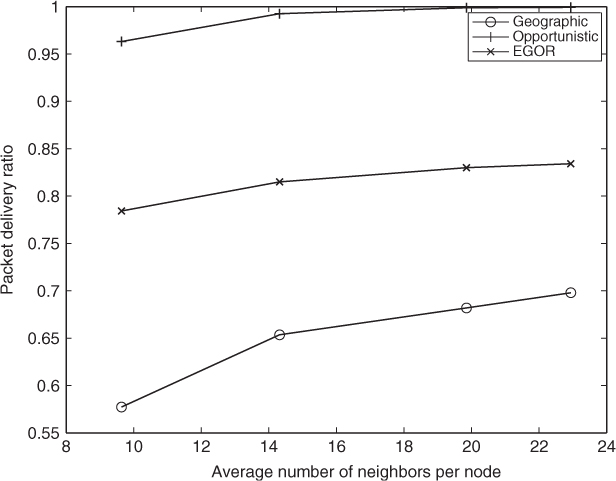
Figure 3.5 Hop count versus network density. Reproduced by permission of © 2007 IEEE.
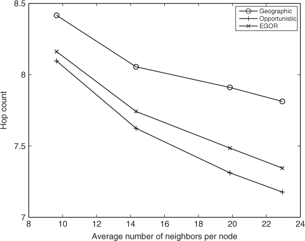
Figure 3.5 also shows that the hop counts decrease when network is denser for all the three protocols, because involving more available next-hop nodes brings more chance for packets to make larger advancement when nodes are uniformly distributed. Opportunistic routing has the smallest hop count under all the node densities, while geographic routing has the largest hop count. Hop count of EGOR is between two of them. From Lemma 2.1 in Section 2.2.1, we know that the maximum EPA, by choosing r nodes from a given set, is strictly increasing with r. So opportunistic routing archives the largest EPA by selecting all the available next-hop nodes as forwarding candidates; geographic routing gets the smallest EPA by choosing only one forwarding candidate, and EGOR archives larger EPA than geographic routing and smaller EPA than opportunistic routing by selecting some (not all) available next-hop nodes as forwarding candidates. Actually, in this simulation, EGOR selects 1.2 nodes on average as the candidate forwarders under each node density. This observation suggests that under such settings, only a few nodes are necessary in order to take advantage of opportunistic routing efficiently. Adding one more node in forwarding can get much better energy efficiency and reliability than geographic routing. Involving all the available next-hop nodes in opportunistic routing is an energy wasteful method.
3.4.2.2 Impact of Reception to Transmission Energy Ratio (RTER)
We study the performance of the three protocols under different RTERs in this section. In the simulations, no retransmission is allowed and the available next-hop node set size is 6.7 on average. The reception power consumption is varied from 10−3 to 10 MW, so the corresponding RTER is in the range [3 × 10⁻⁴, 0.75].
Figure 3.6 shows that the energy efficiency of EGOR is always the best of the three protocols and the RTER is a crucial parameter affecting the energy efficiency of the opportunistic routing. There is a watershed on RTER, smaller than which the energy efficiency of the opportunistic routing is better than the geographic routing, while greater than which the geographic routing surpasses the opportunistic routing. The reason is that when the energy consumption of reception is negligible compared to that of the transmission, the opportunistic routing achieves a larger EPA than the geographic routing while consuming nearly the same energy as geographic routing. So opportunistic routing is more energy efficient. However, when the energy consumption of reception is comparable to transmission, involving all the available next-hop nodes in the opportunistic routing consumes much more energy than the geographic routing and the cost of the increased energy consumption overwhelms the benefit of the increased EPA. Thus, the energy efficiency of the opportunistic routing is less than the geographic routing when RTER is greater than the watershed. For these two protocols, RTER does not affect the forwarding candidate(s) selecting criteria, so it does not affect the PDR.
Figure 3.6 Energy efficiency versus reception to transmission power ratio.

Figure 3.7 shows that the PDR of the geographic routing and opportunistic routing does not change according to the RTER. For EGOR, the PDR decreases when RTER increases because EGOR takes the energy consumption into account. When the reception energy cost increases, fewer nodes are selected as forwarding candidates, then the packet is more likely to be lost without retransmission. An interesting observation here is that, even when RTER is very small, EGOR only selects a very small number of nodes as the forwarding candidate, but achieves nearly the same energy efficiency as opportunistic routing. For example, when RTER = 0.03%, EGOR only selects 2.2 forwarding candidates on average, while it has the same energy efficiency and PDR as the opportunistic routing which selects 6.7 candidates on average. This result again suggests that only a small number of nodes need to be involved in opportunistic routing to achieve a good balance between energy efficiency and routing efficiency.
Figure 3.7 Packet delivery ratio versus reception to transmission power ratio.

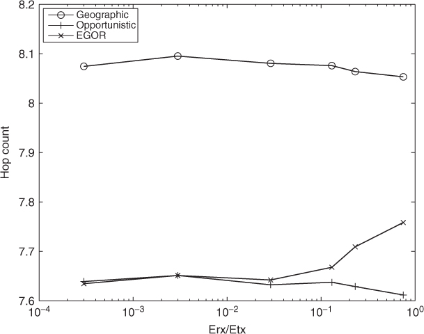
The hop-count performance shown in Figure 3.8 indicates that the RTER does not affect the hop count of the opportunistic routing and geographic routing, the reason is as the same as the PDR performance of these two protocols. For EGOR, the hop count increases after the RTER is larger than 10% because fewer forwarding candidates are selected and the EPA is decreased.
Figure 3.8 Hop count versus reception-to-transmission power ratio.
3.4.2.3 Impact of Retransmission Limit
In this section we study how the retransmission limit affects the performance of the three protocols. The reception power consumption is fixed at 2 MW and the available next-hop node set size is also 6.7 on average.
Intuitively, increasing retransmission limit will increase the reliability, say PDR. Figure 3.9 shows this trend for all the three protocols. It is worth mentioning that the benefit of increasing the retransmission limit (which can be seen as the slopes of the curves) for the opportunistic routing is trivial but for the geographic routing is obvious (especially when retransmission limit is less than 4). The reason is that the opportunistic routing has already achieved a high PDR (nearly 1) by involving all the available next-hop nodes in forwarding even when there is no retransmissions allowed. For the geographic routing, however, there is only one next-hop node involved in the forwarding, then the packet is more likely to be lost in one transmission than in the opportunistic routing. For EGOR, the PDR increasing rate is less than that of the geographic routing because EGOR already achieves higher PDR than the geographic routing when no retransmissions are allowed. When the retransmission limit is larger than 1 the PDR gains become less and less for both EGOR and the geographic routing, and when the limit is larger than 3, the PDRs of both are approaching to 1.
Figure 3.9 Packet delivery ratio versus retransmission limit.
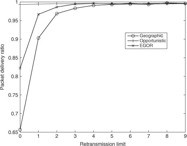
Figure 3.10 shows that, for opportunistic routing, the energy efficiency has not changed much with the change of retransmission limit. The reason is that the retransmission does not play a role for the PDR in opportunistic routing and almost the same packets can be delivered to the destination whether retransmission is allowed or not. For geographic routing and EGOR, the retransmission does play a role for the energy efficiency when retransmission limit is less than 3. As we have analyzed, retransmission affects the PDR, especially from allowing no retransmission to one and from one to two. When retransmission limit is larger than 3, the energy efficiency of these two protocols do not change much as the PDRs are already approaching 1.
Figure 3.10 Energy efficiency versus retransmission limit.

As retransmission does not affect EPA much, Figure 3.11 shows that the hop count remains almost the same when the retransmission limit varies for each of the three protocols.
Figure 3.11 Hop count versus retransmission limit.

3.4.2.4 Number of Local Forwarding Candidates Involved
We study the number of local forwarding candidates involved in opportunistic routing and EGOR under various node densities and RTERs. In the simulations, we use different node numbers (100, 144, 196, 225) to achieve various node densities corresponding to the available next-hop candidate set sizes of 4.6, 6.7, 9.2, 10.5 on average respectively. The RTER is in the range [3 × 10⁻⁴, 0.75].
Figure 3.12 shows the simulation result. Opportunistic routing uses all the available next-hop nodes as the forwarding candidates, whereas EGOR only uses a very small number of forwarding candidates (around two or fewer). For example, even when the RTER is as small as 0.03%, EGOR only chooses 2.2 forwarding candidates on average under various node densities. This means even when the energy consumption of reception is far less than that of transmission, in order to achieve maximum energy efficiency we still only need to involve two forwarding candidates. Figure 3.12 also shows that the number of forwarding candidates is affected mainly by the RTER but not by the node density under a uniform node distribution. For example, when RTER = 0.75, the forwarding candidates in EGOR are nearly unchanged as 1.1 under different node densities. This is an important result as it indicates that involving more forwarding candidates will not bring much more expected packet advancement. A small number of forwarding candidates is sufficient to strike a good balance between EPA and energy consumption. This is a very desirable result because the cost incurred due to assuring one final forwarder from multiple forwarding candidates at the MAC layer is expected to grow when involving more forwarding candidates (Shah et al. 2005). Involving fewer candidates introduces less rendezvous and contention cost.
Figure 3.12 Number of forwarding candidates involved under different node densities and RTERs.

3.4.2.5 Concavity of Maximum EPA and its Slope
In this section, we study the concavity of the maximum EPA function and its slope in one hop under various node densities. The nodes are uniformly distributed and the next-hop available node number varies from 6 to 12. From Figure 3.13 we can see that the maximum EPA increases when the number of the forwarding candidates increases, and when nodes are denser, the EPA is larger. A very interesting result is that under different node densities, the slopes of each curve in Figure 3.13 are nearly the same, which is shown in Figure 3.14. Notice that, when the forwarding candidate number is 3, the slope is already decreased to below 0.01. When the number of forwarding candidates is larger than 4, the slope is near to zero. Figures 3.13 and 3.14 manifest that no matter what the node density is, the EPA gain of involving more forwarding candidates becomes very small when the number of forwarding candidates is larger than 3. These results are consistent with Figure 3.12 where the optimal energy efficiency is achieved when the number of forwarding candidates is around 2.2.
Figure 3.13 Maximum EPA versus forwarding candidate number under different node densities.
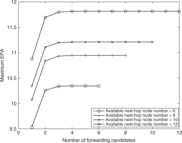
Figure 3.14 EPA slope under different node densities.
