
2
Deep Neural Network Attacks and Defense: The Case of Image Classification
Hanwei ZHANG, Teddy FURON, Laurent AMSALEG and Yannis AVRITHIS
IRISA, University of Rennes, Inria, CNRS, France
Machine learning using deep neural networks applied to image recognition works extremely well. However, it is possible to modify the images very slightly and intentionally, with modifications almost invisible to the eye, to deceive the classification system into misclassifying such content into the incorrect visual category. This chapter provides an overview of these intentional attacks, as well as the defense mechanisms used to counter them.
2.1. Introduction
Deep neural networks have made it possible to automatically recognize the visual content of images. They are very good at recognizing what is in an image and categorizing its content into predefined visual categories. The vast diversity of the many images that are used to train a deep network allows it to recognize visual content with a high degree of accuracy and a certain capacity for generalization. From thousands of examples of images of animals, manufactured objects, places, people, elements of flora, etc., a deep neural network can almost certainly detect that an unknown image shows a dog, a cat, an airplane.
However, it is possible to intentionally modify these images so that the network is completely wrong in its classification. These modifications are made by an attacker whose goal is to deceive the classification, for example to pass off inappropriate content (child pornography) as something perfectly harmless. The big surprise is that these modifications are very small and are almost imperceptible to our eyes. These attacks take advantage of a certain vulnerability of deep networks, which can be quite easy to fool, as we will show in this chapter.
Passing off one piece of visual content for another is very problematic. Putting small pieces of paper of a particular shape and color in certain places on road signs prevents their automatic recognition by dashboard cameras in autonomous vehicles. Wearing a medallion decorated with a particular texture on clothing can make a person invisible to an algorithm detecting the presence of pedestrians. The examples multiply, and are sometimes funny, sometimes disturbing and sometimes dangerous when the decisions of the network puts lives at stake.
Adversarial images that are capable of deceiving classifiers are defined in section 2.2, and an overview of attacks intended to deceive a classifier whose technology is based on deep neural networks is provided in section 2.3. In response, many studies propose defenses, and section 2.4 aims to present them.
We will begin this chapter with a short presentation of the history of the field, and the vocabulary that we will be using. We will also present the main features of machine learning and image classification by deep neural networks.
2.1.1. A bit of history and vocabulary
This chapter deals with the vulnerabilities of deep neural networks, but in fact all machine learning algorithms have flaws and are vulnerable to intentional attacks. It was while researchers were working on automatic email classification in an attempt to separate spam from real messages that the first flaws were revealed. It was the work of Dalvi and his colleagues, and also Lowd and Meek in 2004, that showed that it was possible to deceive a linear classifier trained to detect spam (Dalvi et al. 2004; Lowd and Meek 2005). At that time, deep networks did not exist, and the techniques to choose from for machine learning processes relied on classifiers based on supportvector machines in particular.
Ten years later, the adversarial machine learning sector is gaining momentum, because at the moment the incredible power of deep networks is being revealed, but at the same time they are very vulnerable. Around 2014, researchers were working on making images that could deceive a classifier based on a deep neural network. These images are called “adversarial images”.
Therefore, adversarial images are images that have been manipulated so that the network that classifies them is mistaken and assigns these images to an erroneous class. For example, if a image of a cat is shown, the network responds that this image is of an airplane. However, manipulation is almost invisible and by looking at the manipulated image, it looks exactly like a cat. The network itself is very confident in its decision that it is an airplane. Figure 2.1 illustrates this, where the American flag, when altered intentionally, is recognized as a vending machine, or even a sandal.
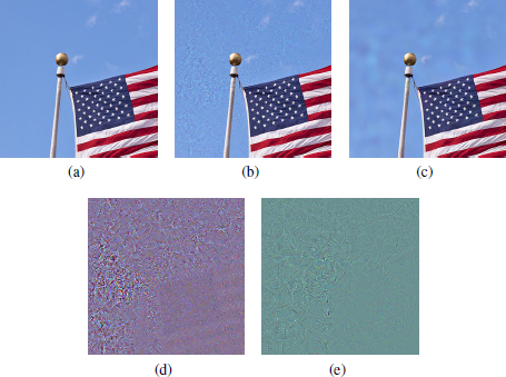
Figure 2.1. The original image and adversarial images; the manipulations are almost invisible, the classification is incorrect
COMMENT ON FIGURE 2.1.– (a) The original image, classified correctly as a flag. (b) An adversarial image, created using the C&W method, classified as a vending machine by the network. (c) An adversarial image, created using the PGD2 method, classified as a sandal by the network. (d) Distortion (greatly amplified to make it more visible) exists in image (b) and is created using C&W, making the original adversarial image. (e) Highly amplified distortion existing in image (c) and created using PGD2, making the original adversarial image.
Historically, one of the first studies into the many facets of vulnerability in learning algorithms was carried out by Barreno et al. (2006). In this seminal article, they discuss the vulnerability of artificial learning algorithms during the learning phases (they discuss poisoning) and the test phases (they discuss evasion), they distinguish between targeted attacks and non-targeted attacks, propose techniques for evaluating the power of these attacks and mention some defense mechanisms to avoid them. They also differentiate vulnerabilities according to the knowledge an attacker may have of the system they want to deceive, distinguishing “white box attacks” from “black box attacks”. We will come back to these terms in section 2.3.
A very good historical perspective can be found in the article by Biggio and Roli (2018). Some excellent recent and complete developments are suggested by Serban and Poll (2018). We recommend reading these two publications.
2.1.2. Machine learning
Machine learning is part of the artificial intelligence field. Machine learning is an interdisciplinary field, with a mix of applied mathematics, statistics and algorithmics. It enables a computer to perform a task based on the careful examination of representative data. The set of rules that the machine must follow in order to perform a task is often either impossible to list “manually” because it is too complex (automatic translation for example), or defined, but leads to an exponential combination of behaviors given all possible input data (chess, go). Machine learning is specifically based on the analysis of huge amounts of data to estimate a model for performing the task. The more data and the more diverse the data, the better the model and the automatic fulfillment of the target task.
Machine learning has two phases. The learning or training phase first learns a model from a set of training data. The second phase applies the learned model to new data and therefore carries out the task. Sometimes, learning and application are intertwined in an effort to continuously improve the quality of the model.
The nature of the information available during the learning phase determines two types of approaches. Supervised learning uses data-label pairs, with the label being the responses we want the task to produce for each data item. It is then a question of classification of the data when the labels have discrete or categorical values, or of regression if they are continuous. On the other hand, non-supervised learning does not have labels. Since it is not always possible to label the large amounts of data, intermediate approaches have been designed where the degree of supervision is more or less high. There are so-called semi-supervised (the data are not all labeled), or even partially supervised (only some of the labels relevant to given data are provided) approaches. There are also other forms of learning, such as reinforcement learning and transfer learning, but we will not go into them in detail here.
The fields of application are extremely varied, as are the tasks to be carried out: classification tasks, recognition tasks, translation tasks, grouping tasks, analysis tasks and prediction tasks; the list is almost endless. Learning applies to data of very different natures: symbolic, digital data, data of a continuous or discrete nature, graphs, trees, feature vectors, including images, sounds, texts and time series for example.
In this chapter, we focus on a specific type of data and the particular task of classifying images into predefined visual categories. The labels are associated with images, for example, airplane, boat, car, table, chair, building, person, dog, cat, ball, cutlery, daisy or tomato. We now consider a supervised learning environment. Once the model has been learned, it is a question of classifying new unknown images, without labels, into the right visual category or categories as best as possible.
Any machine learning process is built on a few fundamental concepts, whether technical or theoretical, that we will detail in this section. First is the concept of an objective function. This very generic term designates a function that reflects the performance of the model; in other words, its ability to perform the intended task. The training optimizes the parameters of the model in order to gradually maximize the objective function. This function is often a decreasing function of a global error linked to the incomplete performance of the task. The opposite of a mean squared error or a cross-entropy are two classic examples of objective functions. These functions are continuous with respect to the parameters of the model and make it possible to detect whether or not a small modification of the parameters improves the performance of the task.
The improvement of the learning is achieved by a gradual adjustment of the parameters of the model, so that the new values of these parameters increase the quality of the model observed through the objective function. Therefore, an optimization process is at work which, we hope, will find the optimum parameters without making the search for them too costly. The adjustment consists of a better positioning of a hyper-plane separating two families of data, for example.
After optimization, the learned model works well on the data used in training, which is normal. However, it is important that this model has generalization capabilities, so that, it can correctly process new and unknown data. Sometimes, when the model over-fits, it has little or no generalization capabilities. This must be avoided, so techniques such as cross-validation, regularization or random pruning could be used.
2.1.3. The classification of images by deep neural networks
This section describes what deep neural networks are and what the image classification task is. This section only provides an overview of these concepts and only presents the most important ones. We invite the reader to study the work by Goodfellow et al. (2016), which presents these concepts in much more detail and precision. In addition, this section introduces the mathematical notations needed to describe attacks and defenses later on.
In the red, green and blue color space, an image I of L lines and C columns is represented by a three-dimensional table in space {0, 1, . . . , 255}3×L×C. The pixels are integers between 0 and 255 (if coded on one byte). The output of the classifier is a class, that is, categorical data. The k possible categories (for example, airplanes, boats, cars, tables, chairs, buildings, people, dogs, cats) are ordered arbitrarily and the output of the classifier is an integer between 1 and k, denoted by ![]() .
.
The image classifying deep neural network here is schematically broken down into three levels. The first layer performs preprocessing that adapts the input image to the neural network. It often includes a sub-sampling of the image to a given size r × r (typically 224 × 224), and mainly reduces the dynamics of the pixels to the range [0, 1] (a historical choice, but other choices are possible, like, for example reducing toward [−1, 1]). This can be done by dividing the pixel value by 255. More sophisticated transfer functions, which are sometimes different from one color channel to another, are also used. The output of this preprocessing is x = T(I), traditionally noted as a column vector at m = 3 × r × r components in [0, 1]m.
The second layer is the neural network. A neuron is a small automaton that combines the data it receives from other neurons, and produces a value which is then transmitted to one or more neurons, which will each combine that value with the values received from other neurons and so on, which makes up an overall network. Neurons are often organized in layers, connected to each other, and it is the great multiplication of these layers that gives the term “deep”. For example, there are networks made up of hundreds of interconnected layers, each made up of thousands of artificial neurons.
Therefore, a neuron is a small automaton that first operates a linear combination of the values received (from other neurons, for example), which are weighted by synaptic weights, and then added up. The value produced is then passed to an activation function, also called a thresholding function. Such functions introduce nonlinearity into the behavior of the neuron, which is essential. Sigmoid activation functions, hyperbolic tangent function, or Rectified Linear Unit (ReLU)-based functions are often used. These nonlinear functions are continuous, non-decreasing and are almost universally differentiable.
The output of the neural network is a real vector at k components called the logit vector: z = R(x, θ) ∈ ![]() k. The larger z(j), the jth logit, is, the more likely the input data x belongs to class j. The θ symbol is a “catch-all” parameter, representing the set of synaptic weights (of all neurons in all layers).
k. The larger z(j), the jth logit, is, the more likely the input data x belongs to class j. The θ symbol is a “catch-all” parameter, representing the set of synaptic weights (of all neurons in all layers).
The third layer translates the logits into a probability vector p ∈ [0, 1]k s.t. ![]() . The value p(j) is the probability that the input image is of class j. This translation is done with the function softmax, p = S(z), defined by, ∀ 1 ≤ j ≤ k:
. The value p(j) is the probability that the input image is of class j. This translation is done with the function softmax, p = S(z), defined by, ∀ 1 ≤ j ≤ k:
It is the gradual adjustment of the synaptic weights θ, parameters of the function R(·), which forms the core of supervised learning, the first and the last layer being non-parametric. These weights are gradually adjusted so that the final value produced at the output of the classifier ultimately corresponds to the label associated with the input data.
The network is used in propagation mode when the input data gradually passes through it, and the network eventually produces the probability vector p. The error between the output p and what should have been produced is measured. For a label ℓ associated with the input x, the output is ideally a probability vector ![]() where
where ![]() and where the other components of this vector are zero. The cross-entropy
and where the other components of this vector are zero. The cross-entropy ![]() is a metric quantifying how p is different to p*. The loss for the input x of the label ℓ is the number
is a metric quantifying how p is different to p*. The loss for the input x of the label ℓ is the number ![]() .
.
Backpropogation consists of tracing the error made by a neuron back through the network, from downstream to upstream, to its synapses and therefore to the upstream neurons. The gradient of the cross-entropy is calculated like this. This is greatly simplified by a chain calculus because the network is a composition of functions or layers. Therefore, the set of these weights θ is updated iteratively by a gradient descent algorithm to decrease the cross-entropy. At iteration i:
where {xj(i), ℓj(i)} corresponds to training data drawn at random at the ith iteration of the stochastic descent gradient and η > 0 is the learning rate.
It is this constant back and forth between propagation (calculated from S(R(x, θ))) and backpropagation (calculated from ![]() ), which ensures the convergence of the learning toward local minimum weights θ of the cross-entropy calculated on the training datasets.
), which ensures the convergence of the learning toward local minimum weights θ of the cross-entropy calculated on the training datasets.
Once the learning is over, the test phase can start. During that phase, unknown data is checked against the model, which eventually produces a probability vector p. The class predicted for the tested data is the one associated with the greatest probability observed in p, that is:
2.1.4. Deep Dreams
A loss ![]() (x, ℓ, θ) is a continuous function with respect to parameters θ of the network, but also to the input data x. In equation [2.2], it is its gradient with respect to θ that appears. What does the opposite of the gradient mean, with respect to x, −∇x
(x, ℓ, θ) is a continuous function with respect to parameters θ of the network, but also to the input data x. In equation [2.2], it is its gradient with respect to θ that appears. What does the opposite of the gradient mean, with respect to x, −∇x![]() (x, ℓ, θ)? It is a three-dimensional table with the same dimension as x, which indicates what tiny modification should be made to x to reduce the loss, that is, so that the input data is even better classified as belonging to the category ℓ.
(x, ℓ, θ)? It is a three-dimensional table with the same dimension as x, which indicates what tiny modification should be made to x to reduce the loss, that is, so that the input data is even better classified as belonging to the category ℓ.
This idea is at the root of Deep Dreams (Tual and Coutagne 2015; Wikipedia 2020), the psychedelic images, which are shown in Figure 2.2. They were built by increasing the structures recognized by a network in a given image and show us what allows it to predict the category ℓ.
These images where the recognized structures are amplified excessively are now part of the folklore of deep convolutional networks. However, this idea of calculating a gradient rather than a variable x is largely used to visually understand and interpret the decisions of neural networks. References in this field include the papers by Yosinski et al. (2015) and Simonyan et al. (2014).
This raises questions about the quantity +∇x![]() (x, ℓ, θ). Added to the variable x, it decreases the probability p(ℓ): this perturbation erases the typical structures of the class ℓ and the resulting image is not as well recognized as being in class ℓ. In the same way, a perturbation −∇x
(x, ℓ, θ). Added to the variable x, it decreases the probability p(ℓ): this perturbation erases the typical structures of the class ℓ and the resulting image is not as well recognized as being in class ℓ. In the same way, a perturbation −∇x![]() (x, ℓ′, θ) with ℓ′ ≠ ℓ increases the probability that the image is in class ℓ′, which can lead to a wrong classification. This is, in fact, the basic idea for generating white box adversarial images.
(x, ℓ′, θ) with ℓ′ ≠ ℓ increases the probability that the image is in class ℓ′, which can lead to a wrong classification. This is, in fact, the basic idea for generating white box adversarial images.
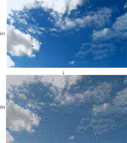
Figure 2.2. Illustration of the Deep Dreams process applied to the original image (a) (source: (Wikipedia 2020))
2.2. Adversarial images: definition
Let f : ![]() → {1, . . . , k} be a classifier mapping a vector of pixels (forming an image) to a discrete label, giving the class that this vector belongs to, among k possible classes. For an image x ∈
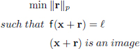
→ {1, . . . , k} be a classifier mapping a vector of pixels (forming an image) to a discrete label, giving the class that this vector belongs to, among k possible classes. For an image x ∈ ![]() and a target label ℓ ∈ {1, · · · , k}, an adversarial perturbation r is produced by resolving the following optimization problem:
and a target label ℓ ∈ {1, · · · , k}, an adversarial perturbation r is produced by resolving the following optimization problem:
This equation fits with targeted and non-targeted attacks, as well as white box or black box attacks.
Targeted attacks are those where the attacker wants to see the attacked image classified exactly in the category ℓ (e.g. the attacker wants an image of a dog to be classified as an image of a cat). Non-targeted attacks are those where the attacker wants an attacked image x + r to be classified in whichever class, as long as ℓ is different from the class f(x) that it belongs to (e.g. the attacker wants an image of a dog to be classified as anything, except a dog).
White box attacks consider the scenario where the attacker knows everything about the classifier network. They can thus imitate it in their garage, assemble it and test an attack, then once operational, they can deploy it. Black box attacks consider the opposite, that the attacker does not know the network details. On the contrary, they have a model of the classifier in their garage. They cannot “open” it and see how it works, but they can use it as an oracle; in other words, submit images to it and observe its predictions as many times as they want to. Certain articles consider “gray boxes”, that is, contexts where the attacker only has partial knowledge of the network. We will come back to all of this later in section 2.3.2.
Equation [2.4] contains a distortion term to be minimized. It is frequently the magnitude of the distortion that is measured, often according to the norm L2, L1, L∞ (Goodfellow et al. 2014a; Carlini and Wagner 2017), since they are quite intuitive, and, when the measure gives a very weak distortion, it is then often almost invisible to the eye. However, these metrics do not reflect our perception of images and small distortions can sometimes be very visible. Also, it is clear that we want to measure the distortion according to another metric, rather than one based on the way our visual system works from a neurological and psychological point of view (Wang et al. 2004; Sharif et al. 2018; Fezza et al. 2019). Unfortunately, this metric is much more complex to calculate. Therefore, the Lp norms are often favored in practice.
Equation [2.4] defines adversial images via an optimization problem. The attack is the process implemented to find the solution to this problem. The variable x existing in a space of a very large dimension m. Finding this solution is difficult since the function f(·) has no explicit form. It is likely that an attack actually finds an approximate solution; in other words, it finds a perturbation r of greater distortion than the bare minimum, given by the solution of equation [2.4]. So a first criterion to evaluate the quality of an attack is the distortion it produces.
A second criterion is given by the second line of equation [2.4]. An attack achieves its goal (targeted or non-targeted) if f(x + r) = ℓ. But this problem is so difficult to resolve that an attack can sometimes fail, failing to produce an adversial image (x+r). So the second criterion to evaluate the quality of an attack is the probability of its success.
These two criteria are deeply linked by a trade-off. It is easy to develop an attack that always succeeds: this attack replaces x by a whole other image x′, whose predicted class is ℓ, but the distortion ‖x′ − x‖p is huge and is clearly visible to the naked eye. It is easy to develop a zero distortion attack: it is the attack which uses the untouched x, but the probability of success is zero (unless x is immediately misclassified by the network). These two extreme attacks are pointless, but they illustrate this trade-off. The probability of success is an increasing function of distortion.
The third criterion is the complexity of the algorithm, measured by its memory consumption or by the required computation time. The algorithms listed below are often iterative, and counting the number of iterations that are needed to make an adversarial image of good visual quality is a valuable indicator. The lower the complexity, the faster the attack, but then the probability of success is often very low or the distortion is very high.
Before presenting different algorithms attacking networks by producing adversarial images, let us come back to the last term of equation [2.4]. It is said that (x + r) is an image. Let us see what this means and what it involves.
This definition, which is based on x = T(I) and not on image I, is historical. It reflects the fact that the community working on computer vision and those working on neural networks are not interested in the preprocessing layer because there is nothing to learn or train. So the condition (x + r) is an image simply means that x + r ∈ [0, 1]m, just like x. It would be possible to come to a “real” digital image (with values of pixels between 0 and 255) by simply applying the inverse preprocessing T−1(·).
In reality, from our point of view, things are not that simple. We have described the preprocessing as being part of the classifier. So x is an internal variable that the classifier does not have access to. However, the aim of the attacker is to attack the input image I, and not x. In addition, the method of first finding x + r, and then applying the inverse preprocessing to form an image is sometimes not possible, because there is no such image such that its preprocessing gives x + r. We will come back to this later in this chapter.
2.3. Attacks: making adversarial images
This section gives a quick overview of techniques used to produce adversarial images. We are not exhaustive, we will describe attacks which are, in a way, exemplary of what the literature offers, very vast literature that is rapidly expanding. All of the techniques presented here are based on equation [2.4], which they enrich in a number of ways.
We mainly describe the case where the network is perfectly known to the attacker (white box attack) and the attacks are not targeted (untargetted attacks). We will extend this framework at a later stage.
2.3.1. About white box
2.3.1.1. The attacker’s objective function
In this scenario, the attacker has access to the probability vector p, calculated by the network. With the original image being from class ℓg, the vector p must move away from ![]() (the image is less recognized as being from class ℓg). In an attack targeting the class ℓ, p must get closer to
(the image is less recognized as being from class ℓg). In an attack targeting the class ℓ, p must get closer to ![]() . Like supervised learning, the attacker also works with an objective function defined via cross-entropy:
. Like supervised learning, the attacker also works with an objective function defined via cross-entropy:
Decreasing the objective function amounts to increasing the predicted probability for the class ℓ and decreasing that of the original class ℓg. Note that a perturbation makes the image adversarial if ![]() .
.
The definition of the objective function is more difficult for non-targeted attacks. Decreasing only ![]() is not enough. The first trick is to target the most probable class, other than ℓg. Hence an objective function:
is not enough. The first trick is to target the most probable class, other than ℓg. Hence an objective function:
There are other objective functions in the literature. We will see, for example, the DeepFool attack, which detects that a predicted high probability class is not necessarily an easier class to reach.
2.3.1.2. Two big families
The core of equation [2.4] is formed by minimizing a distortion and successfully deceiving the system. Also, the algorithms producing adversarial images are divided into two families, according to whether they set themselves the objective of never exceeding a distortion whose maximum value is specified, or the objective of succeeding in producing adversarial images that will all be able to deceive the system, without limiting the distortion (although the minimum is sought). Let us characterize these two families before listing the algorithms.
2.3.1.2.1. Distortion objective
All of the algorithms producing adversarial images included in this family aim to maximize the probability of success while not exceeding a fixed distortion. This distortion is not necessarily an explicit parameter of the attack, but it is determined by some of its parameters. This is generally expressed by:
where ![]() is the lossy function of the attacker and ϵ is the maximum distortion allowed.
is the lossy function of the attacker and ϵ is the maximum distortion allowed.
The performance of this type of attack is measured by their probability of success ![]() , which of course depends on the value given to ϵ. If the attack does not succeed for a given value of ϵ, then this value can be increased and the algorithm starts again with this new, larger ϵ. Note that the ϵ, having finally made it possible to create an adversarial image, is not necessarily minimal.
, which of course depends on the value given to ϵ. If the attack does not succeed for a given value of ϵ, then this value can be increased and the algorithm starts again with this new, larger ϵ. Note that the ϵ, having finally made it possible to create an adversarial image, is not necessarily minimal.
2.3.1.2.2. Success target
In this family, algorithms aim for success and always produce an adversarial image at the cost of arbitrary, but minimal, distortion. This is expressed by:
It is the minimum distortion expectation that characterizes the performance of these algorithms once the network is fooled.
These two families of attacks use a development limited to the first order of the objective function as a basic principle:
The distortions r which decrease the objective function are therefore positioned toward the opposite of the gradient ![]() . This approximation, being local, is only valid for the distortions of low amplitude.
. This approximation, being local, is only valid for the distortions of low amplitude.
From the value of the objective function, a backpropagation process is initiated, which goes back to the vector representing the image while keeping the synaptic weights unchanged. Then, it is this vector that modifies the original image so that the system is eventually fooled. The perturbation is, therefore, a function of the gradient. It is worth noting that because of auto-differentiation (Goodfellow et al. 2016), the calculation of the gradient is automatic. On the other hand, the complexity of this calculation is just double that of the propagation. Let us now list the main algorithms belonging to these two families.
2.3.1.3. Distortion objective: main attacks
2.3.1.3.1. FGSM
The first algorithm that uses the gradient to create a perturbation and produces an adversarial image is the one proposed by Goodfellow et al. (2014a). It is FGSM, which stands for the Fast Gradient Sign Method. This method is very simple and depends on a perturbation calculated as:
It is this perturbation that minimizes the objective function to the first order for the constraint ‖r‖∞ = ϵ.
The characteristic elements of attacks whose objective is distortion are found here (see equation [2.8]). By studying the gradient of the objective function ![]() , and by calculating the opposite, it is then possible to determine how to modify the vector at the input of the network to decrease
, and by calculating the opposite, it is then possible to determine how to modify the vector at the input of the network to decrease ![]() and hopefully lead to its misclassification. The value of ϵ controls the maximum distortion allowed. This method is very simple and very quickly creates adversarial images that can sometimes mislead the classifier. However, it is a bit rough, since it only uses one observation of the gradient to determine which perturbation to apply.
and hopefully lead to its misclassification. The value of ϵ controls the maximum distortion allowed. This method is very simple and very quickly creates adversarial images that can sometimes mislead the classifier. However, it is a bit rough, since it only uses one observation of the gradient to determine which perturbation to apply.
2.3.1.3.2. I-FGSM
It is simple to refine FGSM by having it observe the gradient multiple times as the perturbation is created. So I-FGSM (Kurakin et al. 2016) is the iterative version of FGSM. Contrary to what equation [2.11] allows, the perturbation is not directly calculated. I-FGSM initializes y0 := x and then iterates by increasing the inverse of the gradient each time by α. The recurrence is therefore:
where ![]() is the estimation on the region
is the estimation on the region ![]() (in the minimum sense of the Euclidean space) followed by a term-to-term threshold to stay in the Hypercube [0, 1].
(in the minimum sense of the Euclidean space) followed by a term-to-term threshold to stay in the Hypercube [0, 1].
Here, the region ![]() is the ball
is the ball ![]() norm, center x and radius ϵ > α. Therefore, the first iterations remain inside the ball and the projection is not active, then the iterations calculate perturbations that get out of the hyper ball and the projection brings them back to its surface. This iterative approach is also known as the Basic Iterative Method (BIM) (Papernot et al. 2018).
norm, center x and radius ϵ > α. Therefore, the first iterations remain inside the ball and the projection is not active, then the iterations calculate perturbations that get out of the hyper ball and the projection brings them back to its surface. This iterative approach is also known as the Basic Iterative Method (BIM) (Papernot et al. 2018).
I-FGSM and BIM carry out targeted or non-targeted attacks, and it all depends on the definition of the objective function.
2.3.1.3.3. PGD2
Projected Gradient Descent is also an iterative method, but it projects the gradient on a ball of norm L2, and not on ball of norm L∞ (Madry et al. 2017). Therefore:
where η(x) := x/‖x‖, which is a normalization, according to the norm L2.
The ball L2 used for the projection is B2[x; ϵ], center x and radius ϵ. Once again, the attack does not end when yi touches the ball B2[x; ϵ] for the first time. It continues and seeks to minimize the objective function while remaining on the ball.
2.3.1.3.4. M-IFGSM
Iterative approaches progress along the gradient at a fixed pace, symbolized by α (see equations [2.12] and [2.13]). Adjusting this value is difficult: if it is too small the algorithms will not progress and find an adversarial image because the number of iterations is limited; if it is too large the algorithms will progress quickly, but then the gradient cannot be followed finely, which can create fluctuations.
Approaches such as M-IFGSM (Dong et al. 2018) incorporate a progressive adaptation mechanism for the pace: during the first iterations, it is an advantage to progress rapidly along the gradient. On the other hand, later, it is better to progress in small steps to better follow the gradient and reach a local minimum.
2.3.1.4. Success goal: main attacks
Techniques in this family are typically more expensive. The discovery of a near adversarial image is guaranteed if the complexity is not limited.
2.3.1.4.1. L-BFGS
Szegedy et al. (2013) discuss the problem of creating adversarial images using a Lagrangian formulation. Distortion is no longer a constraint, but is integrated into the objective function:
For a given value of λ > 0, the minimization of the objective function without constraint is carried out using the numerical method BFGS (Broyden–Fletcher–Goldfarb–Shanno). It is an iterative gradient descent method.
A strong value for λ means that the minimum r* of the objective function is not an adverse perturbation, because it has given too much weight to the Euclidean distortion. On the contrary, a value that is too low gives a minimum r*, making ![]() (x + r) very negative and causing a big distortion. This is illustrated by Figure 2.3. Therefore, it is necessary to do a binary search to find an adequate Lagrange multiplier. This means that the program carrying out the attack has two layered iterative loops, which explains its great complexity.
(x + r) very negative and causing a big distortion. This is illustrated by Figure 2.3. Therefore, it is necessary to do a binary search to find an adequate Lagrange multiplier. This means that the program carrying out the attack has two layered iterative loops, which explains its great complexity.

Figure 2.3. Illustration of L-BFGS in 1D
COMMENT ON FIGURE 2.3.– The perturbation r is collinear with the gradient of the objective function. The abscissa is the norm of r. The objective function ![]() (x + r) is given in red. It disappears and becomes negative when r is strong enough to be adverse. The distortion ‖r‖2 is given as black dotted lines, and the function
(x + r) is given in red. It disappears and becomes negative when r is strong enough to be adverse. The distortion ‖r‖2 is given as black dotted lines, and the function ![]() (x + r) + λ * ‖r‖2 is given in blue and magenta for two values of λ. The first value is too small (in blue): the minimum is “far after” the red asterisk; the perturbation is adverse, but of great distortion. The second value is too big (in magenta): the minimum is before the red asterisk; the perturbation is not adverse.
(x + r) + λ * ‖r‖2 is given in blue and magenta for two values of λ. The first value is too small (in blue): the minimum is “far after” the red asterisk; the perturbation is adverse, but of great distortion. The second value is too big (in magenta): the minimum is before the red asterisk; the perturbation is not adverse.
2.3.1.4.2. C&W
The very well-known attack by Carlini and Wagner (2017), noted as C&W later, follows this idea. However, it also deals with the constraint that x + r must remain in [0, 1]m by a change of variable replacing x + r by σ(w), where w ∈ ![]() n and σ(·) :
n and σ(·) : ![]() → [0, 1] is the sigmoid function applied component by component. In addition, for a given λ, C&W uses the numerical method Adam (Kingma and Ba 2015), to find the minimum of an objective function in
→ [0, 1] is the sigmoid function applied component by component. In addition, for a given λ, C&W uses the numerical method Adam (Kingma and Ba 2015), to find the minimum of an objective function in ![]() m:
m:
where μ > 0 is a margin and [x]+ := x if x > 0, 0 if not.
When ![]() (σ(w)) < −μ, the first term becomes zero and the distortion takes σ(w) back toward x, as illustrated by Figure 2.4. This can cause fluctuations around the margin. Again, a binary search is needed to find a good value of λ, hence great complexity.
(σ(w)) < −μ, the first term becomes zero and the distortion takes σ(w) back toward x, as illustrated by Figure 2.4. This can cause fluctuations around the margin. Again, a binary search is needed to find a good value of λ, hence great complexity.
2.3.1.4.3. DDN
Decoupling Direction and Norm (Rony et al. 2019) is an iterative attack, very similar to PGD2, seen here before. The formulation of DDN is:
Here, the projection is carried out on the sphere S2[x; ρi] of radius ρi and center x, even though yi+1 is inside. The main difference with the PGD2 formulation given by equation [2.13] is that the radius of this sphere changes from one iteration to another. This radius at iteration i is obtained by calculating ρi = (1 − γ)‖yi – x‖ when yi is an adverse vector. When this is not the case, then ρi = (1 + γ)|yi – x‖, with γ ∈ (0, 1).
2.3.1.5. Other attacks
Other attacks are in the same style, but with variations, either on the definition of the objective function, or on the definition of the distortion. Finally, this overview of attacks ends with the description of a few techniques that take quite different paths to achieve their goals. They are separate because it is not easy to arrange them in one of the two families presented above.
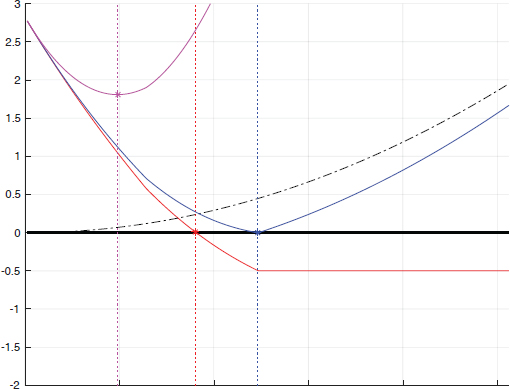
Figure 2.4. Illustration of C&W in 1D. The perturbation r is collinear to the gradient of the objective function. This is the same configuration as in Figure 2.3, except the margin μ = 0.5 for the threshold of equation [2.15]. Notice its effect: the blue minimum is closer to the red asterisk

Figure 2.5. Illustration, in two dimensions, of adverse attacks on a binary classifier
COMMENT ON FIGURE 2.5.– From left to right: PGD2, C&W, DDN. The regions associated with the two classes are in red and blue. The level lines indicate the predicted probabilities. The objective is to find an adverse point in the red area, which is as close as possible to the starting point x. In gray (respectively black), are the paths taken for PGD2 (Kurakin et al. 2016) (radius of the green circle) or for a parameter λ for C&W (Carlini and Wagner 2017).
2.3.1.5.1. DeepFool
It is a non-targeted white box attack that uses a more sophisticated objective function. In equation [2.7], a non-targeted attack uses the objective function in order to assign the most likely class for the classifier to the adversarial image under construction, apart from the original class ℓg. So, the objective function has a positive, but low, value in x. It seems easier to make it negative.
With DeepFool, Moosavi-Dezfooli shows that this reasoning is incorrect. The ease of making the objective function negative certainly depends on its initial value, but also on its gradient. At the first order, according to equation [2.10], the minimum distortion necessary in the L2 norm is achieved when r ∝ −∇x![]() (x, ℓ) with:
(x, ℓ) with:
It is best to target the ℓ class that requires the least distortion. This is illustrated by Figure 2.6. But this formula is only an approximation at the first order. In addition, it must be estimated for all (or part of) the classes, except for the original class ℓg.
2.3.1.5.2. ILC
The Iterative Least-likely Class (ILC) (Papernot et al. 2018) proposes another alternative objective function. It is possible that the class assigned to the attacked image is sometimes semantically close to the original class ℓg. An image of a swallow taken for an image of a sparrow seems more insignificant to us than if this same image of a swallow is taken for an image of a car. Thus, ILC prefers to target the least likely class for the original image.
2.3.1.5.3. JSMA
Papernot et al. (2016b) propose a targeted attack for low distortions in norm L0. The attack finds out which pixels play an important role in the classification. This approach, called the Jacobian-based Saliency Map Attack (JSMA), estimates the Jacobian matrix of the function x → p. This calculation determines which elements of x have the most influence, not only to increase the predicted probability of the targeted class p(ℓ), but also to decrease the predicted probabilities of all of the other classes.
Few pixels have this property, but modifying them is extremely effective in deceiving the classifier. However, they must be modified with a large amplitude, which produces “salt and pepper noise” in the image. This modification is often very visible, but can pass for an error in the coding of the photo.
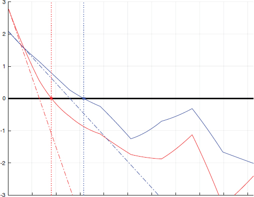
Figure 2.6. Illustration of DeepFool
COMMENT ON FIGURE 2.6.– The blue and red curves correspond to the objective function ![]() (x, ℓ) for two classes ℓ1 and ℓ2, which are different when the perturbation r is collinear with their gradient. The abscissa corresponds to the r norm. Notice that p(ℓg) = 0.8, p(ℓ1) = 0.1, p(ℓ2) = 0.05. As p(ℓ1) > p(ℓ2), it seems interesting to target the class ℓ1: the blue objective function starts from lower down. This is an error because this one is canceled “later” than that of the class ℓ2 in red. To find out, DeepFool calculates the gradient in x, which amounts here to approaching the objective function by its tangent in ‖r‖ = 0 (dotted).
(x, ℓ) for two classes ℓ1 and ℓ2, which are different when the perturbation r is collinear with their gradient. The abscissa corresponds to the r norm. Notice that p(ℓg) = 0.8, p(ℓ1) = 0.1, p(ℓ2) = 0.05. As p(ℓ1) > p(ℓ2), it seems interesting to target the class ℓ1: the blue objective function starts from lower down. This is an error because this one is canceled “later” than that of the class ℓ2 in red. To find out, DeepFool calculates the gradient in x, which amounts here to approaching the objective function by its tangent in ‖r‖ = 0 (dotted).
This technique is remarkable since it is quite fascinating to note that changing the value of a few pixels, or even a single pixel, is enough to lead to a misclassification.
2.3.1.5.4. Universal attacks
Moosavi-Dezfooli et al. (2017) have shown that it is possible to create a unique adversarial perturbation that works whatever the image proposed to the network. To do this, they repeatedly apply the DeepFool algorithm (see section 2.3.1.5.1) to all of the images in the training set until a particular perturbation causes the misclassification of a large part of these images. More formally, their approach looks for the perturbation r, bounded by ϵ, such that:
where δ indicates the proportion of images from the training set that have become adversarial images and belong to the sample Pdata of all of the images.
Generally, the algorithm succeeds in finding multiple adversarial samples, which are often visually very different from each other, thus facilitating universal attacks.
2.3.1.5.5. Geometric attacks
So far, attacks change pixels’ value additively: y = x + r. They are sometimes called value-metric attacks. Geometric attacks do not change the value of the pixels but their position, by slight rotations and local translations. An optical flow applies a displacement field to the pixels of the original image: the pixel at position (k, l) is moved to position (k, l) + Δ(k, l) in the adversarial image.
Xiao et al. (2018) sought to optimize this optical flow by observing the variations in classification probabilities. The objective function integrates ![]() (x, ℓ) and a part regularizing the optical flow so that it generates small continuous movements. Again, a BFGS-type numerical method is used. The adversarial images often seem perfect.
(x, ℓ) and a part regularizing the optical flow so that it generates small continuous movements. Again, a BFGS-type numerical method is used. The adversarial images often seem perfect.
2.3.1.5.6. Generative Adversarial Network attacks
Generative Adversarial Networks (GAN) (Goodfellow et al. 2014b) form a class of machine learning algorithms that learn to estimate a probability distribution from samples submitted to them. The learned distribution forms a model that the network can then use to generate new samples that are completely synthesized, but that will belong to this same distribution. By consuming a very large collection of images of the faces of existing people, a generative network can then synthesize new artificial, but realistic, faces.
GAN are made of two distinct parts, a generator that learns the distribution and generates a new sample, and a discriminator that estimates whether the sample it observes comes from the generator or directly from the learning set, and then notifies the generator. These two parts compete against each other, in that the generator tries to create an artificial sample that the discriminator will not be able to distinguish from a real sample. The discriminator, therefore, forces the generator to improve the quality of the synthesis.
From this general idea, it then seems natural to use these GAN to produce adversarial images. The generator creates adversarial images that nevertheless appear normal to our eyes. Baluja and Fischer (2017), for example, trained a generator to create images, which mislead a particular network by modifying them via a residual network (He et al. 2016).
We are, therefore, very far from the gradient calculation mechanism of the first attacks. The advantage of that generative approach is the almost instantaneous speed to produce an adversarial image. But there are many drawbacks. The learning time is very long. This approach therefore only makes sense if the attacker has a large number of adversarial images to create. In addition, a learned network only targets a given class and is only valid against a particular classifier.
2.3.2. Black or gray box
The black box model is much more strict than the white box model. The attacker does not know anything about the targeted network. At this point, it is impossible to calculate gradients and therefore impossible to apply the techniques mentioned so far. Nevertheless, the attacker can use the targeted network as an oracle and observe the way in which it labels an image that is proposed.
The gray box and black box models assume that the attacker has much less information at their disposal. For the gray box model, we suppose that the attacker knows some elements of the targeted network. For example, that the network uses a pre-trained model made available off the shelf, but with defense mechanisms that are secret. The attacker can then partly reproduce the behavior of the targeted network to set up their attacks.
2.3.2.1. Two concepts about the black box
If the “black box” means observing the inputs/outputs of a system, what are these outputs? Some believe that the output that the attacker has access to is the predicted probability vector p. Others believe that the output is the predicted class ℓ = f(x).
The nature of these outputs makes a big difference, as noted in the article by Ilyas et al. (2018). The predicted class f(x) is a constant piecewise function. Almost certainly, the attacker does not see if a small amplitude perturbation r is going in the right direction, since it does not necessarily change the output. This is not the case for the predicted probability vector.
2.3.2.2. Output = probability vector
In this case, there is no big difference with white box attacks. The attacker calculates an objective function, like in section 2.3.2.1, and seeks a perturbation that minimizes it. The only difference is that unfortunately, the gradient is no longer available. The attacker then uses so-called zero order numerical methods, such as differential evolution algorithms (Storn and Price 1997), sometimes called genetic algorithms. These algorithms randomly take distortions, calculate their objective functions, select the distortions which have obtained the lowest values and recombine them with random mutations. This selection–recombination–mutation cycle is repeated.
In this way, the One pixel attack (Su et al. 2017) is the counterpart of the JSMA attack, where the pixels (even the pixel) to be modified are found thanks to the genetic algorithm. Likewise, Engstrom’s work (Engstrom et al. 2017) is the black box counterpart of the geometric attacks by Xiao et al. (2018) in white box. Likewise, Zhao et al. (2017) involve generators of adversarial distortions, like in Baluja and Fischer (2017), where the discriminator is a black box classifier.
An alternative to genetic algorithms is estimating the gradient of the objective function in certain directions:
To estimate the gradient, we have to calculate this deviation for all of the pixels 1 ≤ i ≤ m, which is costly. Chen et al. (2017) show that this is not necessary. They apply a stochastic gradient descent where the directions ei are iteratively drawn at random. This attack is called zeroth-order optimization (ZOO). Let us quote another attack belonging to this category, designed by Narodytska and Kasiviswanathan (2017).
2.3.2.3. Output = predicted class
Szegedy et al. (2013) are among the first to realize that adversarial images designed to attack one specific network are also adversarial for another network. But it was Papernot et al. (2016a) who first explored the transfer properties of attacks by studying gray box and black box attacks. Let us also cite the work of Liu et al. (2016) as a notable article on this subject. A similar phenomenon, traditional in machine learning, is well known: it is possible, to a certain extent, to transfer what has been learned by one network to another.
Papernot et al. (2016) rely on the observation of the proportion of adversarial images deceiving the first system, which also succeed in deceiving the second. To be more precise, they distinguish transfers between learning systems built on the same fundamental principle from transfers between systems built on different principles (a transfer between a deep network and an SVM-based system for example).
The results of their study (Papernot et al. 2016a) show that the transfers are possible and easy between neural systems. On the other hand, although always possible, the transfer of attacks is more difficult between systems built on models that cannot be derived, mathematically speaking, like those built from SVMs, nearest neighbors or decision trees (this is opposed, for example, to neural networks, for which it is easy to calculate the gradient).
This observation then makes it possible to attack black box learning systems. By multiplying the requests to the targeted classifier, the attacker can build a model: a new classifier is trained to imitate the black box in the sense that the outputs of this surrogate classifier must ultimately be identical to those of the targeted black box. Then, the attacker uses this new model, but in a white box, to forge adversarial images, with the hope that they also deceive the black box network because of the transfer property.
2.4. Defenses
There are just as many defenses as there are attacks. This section provides an overview. Schematically, we can distinguish three families of defenses:
- – Reactive techniques: these strategies are based on preprocessing, carried out before feeding the network. These block the images if adversarial content is detected or filter and clean the images, hoping to remove the adversarial perturbation.
- – Proactive techniques: these strategies build networks that are inherently stronger to adversarial attacks. This category includes, for example, approaches which incorporate many adversarial images into the learning phase.
- – Obfuscation techniques: these strategies hide or obfuscate the important parameters that an attacker needs to produce adversarial images.
Another viable view distinguishes whether the defense is an add-on module connected to the network (and therefore the classifier works with or without defense), or whether the defense is an integral part of the network resulting in a radical transformation of the classifier.
2.4.1. Reactive defenses
This family groups together the techniques which detect the adversarial nature of an image and/or apply a preprocessing to the images submitted to the network, to eliminate what makes them adversarial from their content.
Detection techniques introduce an additional class. This class is not necessarily labeled “adversarial images”, but simply “unknown class”. The fundamental theory is that the goal of the attacker is not to target this class. The attack fails if this class is the result of classification. The detection is sometimes justified as follows: (1) the images are points in a large-dimensional space ![]() m concentrated along manifolds; (2) attacks push these images out of their manifold. The detectors learn to distinguish these manifolds by collecting statistics, calculated either in the image domain, or in the hidden layers.
m concentrated along manifolds; (2) attacks push these images out of their manifold. The detectors learn to distinguish these manifolds by collecting statistics, calculated either in the image domain, or in the hidden layers.
The preprocessings filter the images in order to remove the adversarial distortion, without altering the visual content. Here, the images are never rejected, we hope they are cleaned and therefore harmless. In theory, filtering amounts to projecting an image onto the manifolds of the natural images mentioned above. Once again, some techniques filter the images before classification, others filter the representations that travel in the networks.
In reality, reactive techniques mix preprocessing and detection. It is possible to build a detector from preprocessing by thresholding the quantity of the filtered noise of the image. Therefore, we list examples of reactive defenses without clear distinction.
2.4.1.1. Learn about the manifold of natural images
This is the issue for many defenses. The advantage is that this learning only consumes original images. Thus, the defense is not biased toward one or more specific attacks. MagNet (Meng and Chen 2017) employs autoencoders to project the image and bring it closer to the manifold of natural images. Variants use sparse representations of image patches like D3 (Moosavi-Dezfooli et al. 2018), estimates based on mixtures of Gaussians (Ghosh et al. 2018), or deep generator networks like PixelDefend (Song et al. 2017) or Defense-GAN (Samangouei et al. 2018). More uncommon, Dubey et al. (2019) search the Internet for the images most similar to the query, then decide on its class by a majority vote on the predictions of the similar images.
2.4.1.2. Interaction with the classifier
A simple method of detection is feature squeezing (Xu et al. 2017). Many simple filters are applied to degrade or simplify the image, hence the name “squeezer” (compression, slight blur filter), before submitting it to the network. Then, the deviations at the output of the network are observed with respect to the predicted probability vector p given for the original image. Any significant deviation suggests that the tested image is adversarial. Guo et al. (2017) and Liang et al. (2018) developed approaches that are very close one another. SafetyNet (Lu et al. 2017) is based on the analysis of active neurons in the classifier. They encode typical activation patterns of a deep layer of a network processing clean images, and compare this description to the current one when an unknown image is processed. This comparison is made via a radial kernel support vector machine. Bypassing this defense forces the attacker to integrate the response of all of the rectification units in the network into their attack, which is difficult in practice. This defense works well, even when the network is big. A more recent version of this defense idea is called Network Invariance Checking (Ma et al. 2019).
2.4.2. Proactive defenses
Proactive defenses aim to improve the intrinsic strength of models.
2.4.2.1. Reducing the amplitude of gradients
If the network function experiences strong gradients, then a very small perturbation is needed to greatly modify the output of the network. This explains the vulnerability of the network to attacks. Reducing the amplitude of the gradients makes the network stronger.
One of the very first approaches is “distillation”, which is originally a technique for transferring what has been learned by a large network to a smaller network (Hinton et al. 2015). In very broad terms, the distillation trains the small network, not with the labels of the images, but with the probability vectors predicted by the large network, which are more informative than simple labels. Papernot et al. (2016c) rely on distillation, but apply this transfer on the same network architecture. Therefore, the first version of the network is trained on labels, and the second is trained on the knowledge learned from the first. This “autotransfer” is made at a high temperature in the softmax function, which reduces the amplitude of the gradients of the network function. Nevertheless, Carlini and Wagner designed attacks that made the distillation defenses fail (see the C&W attack, in section 2.3.1.4).
Gu and Rigazio (2014) suggest training networks with a new constraint: each layer must be “contracting”, in the sense of a Lipschitzian function (Tsuzuku et al. 2018). This is incorporated during the training by a penalty, which aims to reduce the variation of its response to perturbations it receives as an input. Overall, this increases the strength of the network and requires the applied distortion to be significantly stronger for an attack to be successful.
2.4.2.2. Adversarial training
Learning with more data allows a network to generalize better, to refine the boundaries between classes in the representation space. This classic trick is done by adding quasi copies of images that have undergone small translations or rotations.
The idea is the same here, by improving learning with adversarial images. The network therefore learns that, despite the perturbation, such-and-such an image is indeed in such-and-such a category. The principle is simple, but the implementation is difficult. An attack targets a network, which during the learning process is, by definition, unpredictable. Each time the synaptic weights are updated, the adversarial versions of the training images must be recalculated. The attack must therefore be super fast. This is how Goodfellow et al. (2014a) proceed thanks to the simplest of attacks: FGSM.
This idea leads to the concept of robust optimization by a min–max formulation, where the learning process has an objective:
with {xj, ℓj} training data.
In a way, the training tries to get all of the images in the ball with center xj and radius ϵ to be classified as xj. We can also cite various works exploring these same ideas (Huang et al. 2015; Madry et al. 2017; Tramèr et al. 2017). Let us quote the approach by Lee et al. (2017) again, where a generative network creates adversarial images, which feed a classifier carrying out adversarial learning.
Many gray areas remain in adversarial training. The robustness provided is sometimes disputed. The network is more robust against simple attacks, but still just as vulnerable to more complex attacks. The robustness is obvious on the training images, but it does not generalize well. There is a price to pay: the network is more robust against attacks but less precise on the original images. The consensus is not yet established with certainty because the adversarial training is difficult to carry out. Many variations exist, gradually increasing the quantity of adversarial images, while increasing the strength of the attacks from a very large number of original images. All of this is costly, with the benefits not always outweighing the extra costs.
2.4.3. Obfuscation technique
Creating adversarial images in white box relies most often on the utilization of the gradient of the differentiable objective function. Introducing strong nonlinearities makes the network non-differentiable and prevents the calculation of a gradient. This family of techniques was explored by Goodfellow et al. (2014a) (see Buckman et al. (2018)). Athalye et al. (2018) have explored this subject and show the ineffectiveness of this approach: in white box, nothing forces the attacker to use the gradient of the objective function. It can modify the network and replace any nonlinearity with a smoother function.
Obfuscation becomes more serious when it is based on the insertion of a secret key in the classifier, like in cryptography. This is the only way to prevent white box analysis. The attacker knows all of the details of the network except one secret high entropy parameter. This is difficult to combine with machine learning and often requires re-training the whole network, or part of it, each time a secret key is taken (Shumailov et al. 2018; Taran et al. 2020).
Another possibility is to make the classifier random. For each call to the network, the final prediction depends on a random value that the attacker cannot know. This could be a slight modification to the input image, or modifications within the network: Dhillon et al. (2018) suggest randomly suppressing certain neurons (those which react weakly) and to increase, in proportion, the importance of the reaction of the conserved neurons.
2.4.4. Defenses: conclusion
We have mentioned several defenses; there are many others, sometimes simple variations, and sometimes more original contributions too. In general, the evaluation of their effectiveness leaves a lot to be desired. Many of them are evaluated on very small sets of tests, can only withstand a particular class of attacks without being clearly perceptible, or are even too expensive to be usable in practice. There is not yet a rigorous protocol to assess the quality of a defense technique making a network more robust to adversarial attacks. It is very difficult to compare the respective merits of different defensive strategies.
The addition of defense strategies sometimes leads to a reduction in the quality of the networks: the classification performance on the natural images (not attacked) of a network with defense is worse than without a defense. This observation is disputed because nothing completely implies such tension (although some theoretical papers claim otherwise).
Some approaches take a more formal point of view and try to guarantee the robustness of the network, as long as the distortion remains below a boundary, whose value must be calculated. Still at an early stage, we nevertheless cite the promising studies (Huang et al. 2017; Katz et al. 2017; Sinha et al. 2017; Wong and Kolter 2017; Raghunathan et al. 2018; Ruan et al. 2018). Another contribution, written in French, tackles the same topic (Bazille et al. 2019)
2.5. Conclusion
This chapter has provided an overview of attack and defense techniques, involving the vulnerabilities of machine learning systems based on deep neural networks for image recognition tasks. This field of research is very active and the work is increasing every day.
They aim to make attacks more and more imperceptible (Zhang et al to appear), even when examined through sophisticated psycho-visual metrics (Fezza et al. 2019). They also aim to be faster in order to make defenses based on robust learning (Zhang et al. 2019).
Some works aim to better understand the causes of attacks and the reasons for the success or failure of defenses. Instead, these works explore problems linked to the distribution of data in high-dimensional spaces, the effects of thresholding functions and the theoretical guarantees that a network can offer.
Of course, attacks and defenses are not limited to just images, and some work explores the creation of adversarial videos (Jiang et al. 2019; Wei et al. 2019), audio (Carlini and Wagner 2018; Qin et al. 2019), texts (Behjati et al. 2019) and time series (Fawaz et al. 2019), in an attempt to understand the relationships between vulnerabilities and multimodal data (Park et al. 2019), or even explore the problems of deceiving malware (Martins et al. 2020).
Additionally, other works consider different tasks, such as similarity search (Amsaleg et al. 2017), clustering, feature selection, embedding, hashing, similarity learning and outlier detection.
Much remains to be understood, it is very encouraging.
2.6. References
Amsaleg, L., Bailey, J., Barbe, D., Erfani, S.M., Houle, M.E., Nguyen, V., Radovanovic, M. (2017). The vulnerability of learning to adversarial perturbation increases with intrinsic dimensionality. In Workshop on Information Forensics and Security. IEEE, Rennes, 1–6.
Athalye, A., Carlini, N., Wagner, D. (2018). Obfuscated gradients give a false sense of security: Circumventing defenses to adversarial examples [Online]. Available at: https://arxiv.org/abs/1802.00420.
Baluja, S. and Fischer, I. (2017). Adversarial transformation networks: Learning to generate adversarial examples [Online]. Available at: https://arxiv.org/abs/1703.09387.
Barreno, M., Nelson, B., Sears, R., Joseph, A.D., Tygar, J.D. (2006). Can machine learning be secure? In AsiaCCS. ACM, Taipei, 16–25.
Bazille, H., Fabre, E., Genest, B. (2019). Certification formelle des réseaux neuronaux profonds : un état de l’art en 2019. AI and Defense 2019 – Artificial Intelligence and Defense, 1–10 [Online]. Available at: https://hal.archives-ouvertes.fr/hal-02350253.
Behjati, M., Moosavi-Dezfooli, S., Baghshah, M.S., Frossard, P. (2019). Universal adversarial attacks on text classifiers. In ICASSP. IEEE, Brighton, 7345–7349.
Biggio, B. and Roli, F. (2018). Wild patterns: Ten years after the rise of adversarial machine learning. Pattern Recognition, 84, 317–331.
Buckman, J., Roy, A., Raffel, C., Goodfellow, I. (2018). Thermometer encoding: One hot way to resist adversarial examples. In International Conference on Learning Representations. ICLR, Vancouver.
Carlini, N. and Wagner, D.A. (2017). Towards evaluating the robustness of neural networks. In Symposium on Security and Privacy. IEEE, San Jose.
Carlini, N. and Wagner, D.A. (2018). Audio adversarial examples: Targeted attacks on speech-to-text. In IEEE Symposium on Security and Privacy Workshops. IEEE, San Francisco, 1–7.
Chen, P.-Y., Zhang, H., Sharma, Y., Yi, J., Hsieh, C.-J. (2017). ZOO: Zeroth order optimization based black-box attacks to deep neural networks without training substitute models. In Workshop on Artificial Intelligence and Security. ACM, New York, 15–26.
Dalvi, N.N., Domingos, P.M., Mausam, Sanghai, S.K., Verma, D. (2004). Adversarial classification. In KDD. ACM, Seattle, 99–108.
Dhillon, G.S., Azizzadenesheli, K., Lipton, Z.C., Bernstein, J., Kossaifi, J., Khanna, A., Anandkumar, A. (2018). Stochastic activation pruning for robust adversarial defense [Online]. Available at: https://arxiv.org/abs/1803.01442.
Dong, Y., Liao, F., Pang, T., Su, H., Zhu, J., Hu, X., Li, J. (2018). Boosting adversarial attacks with momentum. In Conference on Computer Vision and Pattern Recognition. IEEE, Salt Lake City, 9185–9193.
Dubey, A., van der Maaten, L., Yalniz, Z., Li, Y., Mahajan, D. (2019). Defense against adversarial images using web-scale nearest-neighbor search. In Conference on Computer Vision and Pattern Recognition. IEEE, Long Beach, 8767–8776.
Engstrom, L., Tran, B., Tsipras, D., Schmidt, L., Madry, A. (2017). A rotation and a translation suffice: Fooling CNNs with simple transformations [Online]. Available at: https://arxiv.org/abs/1712.02779.
Fawaz, H.I., Forestier, G., Weber, J., Idoumghar, L., Muller, P. (2019). Adversarial attacks on deep neural networks for time series classification. In IJCNN. IEEE, Budapest, 1–8.
Fezza, S.A., Bakhti, Y., Hamidouche, W., Déforges, O. (2019). Perceptual evaluation of adversarial attacks for CNN-based image classification. In Eleventh International Conference on Quality of Multimedia Experience. QoMEX, Berlin, 1–6.
Ghosh, P., Losalka, A., Black, M.J. (2018). Resisting adversarial attacks using Gaussian mixture variational autoencoders [Online]. Available at: https://arxiv.org/abs/1806.00081.
Goodfellow, I.J., Shlens, J., Szegedy, C. (2014a). Explaining and harnessing adversarial examples [Online]. Available at: https://arxiv.org/abs/1412.6572.
Goodfellow, I., Pouget-Abadie, J., Mirza, M., Xu, B., Warde-Farley, D., Ozair, S., Courville, A., Bengio, Y. (2014b). Generative adversarial nets. Advances in Neural Information Processing Systems, 27, 2672–2680.
Goodfellow, I., Bengio, Y., Courville, A. (2016). Deep Learning. MIT Press [Online]. Available at: http://www.deeplearningbook.org.
Gu, S. and Rigazio, L. (2014). Towards deep neural network architectures robust to adversarial examples. In International Conference on Learning Representations. ICLR, Banff.
Guo, C., Rana, M., Cisse, M., van der Maaten, L. (2017). Countering adversarial images using input transformations [Online]. Available at: https://arxiv.org/abs/1711.00117.
He, K., Zhang, X., Ren, S., Sun, J. (2016). Deep residual learning for image recognition. In Conference on Computer Vision and Pattern Recognition. IEEE, Las Vegas, 770–778.
Hinton, G., Vinyals, O., Dean, J. (2015). Distilling the knowledge in a neural network [Online]. Available at: https://arxiv.org/abs/1503.02531.
Huang, R., Xu, B., Schuurmans, D., Szepesvári, C. (2015). Learning with a strong adversary [Online]. Available at: https://arxiv.org/abs/1511.03034.
Huang, X., Kwiatkowska, M., Wang, S., Wu, M. (2017). Safety verification of deep neural networks. In International Conference on Computer Aided Verification. CAV, Heidelberg, 3–29.
Ilyas, A., Engstrom, L., Athalye, A., Lin, J. (2018). Black-box adversarial attacks with limited queries and information. Proceedings of Machine Learning Research, 80, 2142–2151.
Jiang, L., Ma, X., Chen, S., Bailey, J., Jiang, Y. (2019). Black-box adversarial attacks on video recognition models. In ACM Multimedia. ACM, Nice, 864–872
Katz, G., Barrett, C., Dill, D.L., Julian, K., Kochenderfer, M.J. (2017). Reluplex: An efficient SMT solver for verifying deep neural networks. In International Conference on Computer Aided Verification. CAV, Heidelberg, 97–117.
Kingma, D. and Ba, J. (2015). Adam: A method for stochastic optimization [Online]. Available at: https://arxiv.org/abs/1412.6980.
Kurakin, A., Goodfellow, I., Bengio, S. (2016). Adversarial examples in the physical world [Online]. Available at: https://arxiv.org/abs/1607.02533.
Lee, H., Han, S., Lee, J. (2017). Generative adversarial trainer: Defense to adversarial perturbations with GAN [Online]. Available at: https://arxiv.org/abs/1705.03387.
Liang, B., Li, H., Su, M., Li, X., Shi, W., Wang, X. (2018). Detecting adversarial image examples in deep neural networks with adaptive noise reduction. IEEE Transactions on Dependable and Secure Computing, 18(1), 72–85.
Liu, Y., Chen, X., Liu, C., Song, D. (2016). Delving into transferable adversarial examples and black-box attacks [Online]. Available at: https://arxiv.org/abs/1611.02770.
Lowd, D. and Meek, C. (2005). Adversarial learning. In KDD. ACM, Chicago, 641–647.
Lu, J., Issaranon, T., Forsyth, D. (2017). Safetynet: Detecting and rejecting adversarial examples robustly. In International Conference on Computer Vision. IEEE, Venice, 446–454.
Ma, S., Liu, Y., Tao, G., Lee, W., Zhang, X. (2019). NIC: Detecting adversarial samples with neural network invariant checking. In 26th Annual Network and Distributed System Security Symposium. NDSS, San Diego.
Madry, A., Makelov, A., Schmidt, L., Tsipras, D., Vladu, A. (2017). Towards deep learning models resistant to adversarial attacks [Online]. Available at: https://arxiv.org/abs/1706.06083.
Martins, N., Cruz, J.M., Cruz, T., Abreu, P.H. (2020). Adversarial machine learning applied to intrusion and malware scenarios: A systematic review. IEEE Access, 8, 35403–35419.
Meng, D. and Chen, H. (2017). Magnet: A two-pronged defense against adversarial examples. In SIGSAC Conference on Computer and Communications Security. ACM, Dallas, 135–147.
Moosavi-Dezfooli, S.-M., Fawzi, A., Fawzi, O., Frossard, P. (2017). Universal adversarial perturbations. In CVPR. IEEE, Hawaii, 86–94.
Moosavi-Dezfooli, S.-M., Shrivastava, A., Tuzel, O. (2018). Divide, denoise, and defend against adversarial attacks [Online]. Available at: https://arxiv.org/abs/1802.06806.
Narodytska, N. and Kasiviswanathan, S. (2017). Simple black-box adversarial attacks on deep neural networks. In Conference on Computer Vision and Pattern Recognition Workshops. IEEE, Honolulu, 1310–1318.
Papernot, N., McDaniel, P., Goodfellow, I. (2016a). Transferability in machine learning: From phenomena to black-box attacks using adversarial samples [Online]. Available at: https://arxiv.org/abs/1605.07277.
Papernot, N., McDaniel, P., Jha, S., Fredrikson, M., Celik, Z.B., Swami, A. (2016b). The limitations of deep learning in adversarial settings. In European Symposium on Security and Privacy. IEEE, Saarbrücken.
Papernot, N., McDaniel, P., Wu, X., Jha, S., Swami, A. (2016c). Distillation as a defense to adversarial perturbations against deep neural networks. In European Symposium on Security and Privacy. IEEE, Saarbrücken.
Papernot, N., Faghri, F., Carlini, N., Goodfellow, I., Feinman, R., Kurakin, A., Xie, C., Sharma, Y., Brown, T., Roy, A., Matyasko, A., Behzadan, V., Hambardzumyan, K., Zhang, Z., Juang, Y.-L., Li, Z., Sheatsley, R., Garg, A., Uesato, J., Gierke, W., Dong, Y., Berthelot, D., Hendricks, P., Rauber, J., Long, R. (2018). Technical report on the CleverHans v2.1.0 adversarial examples library [Online]. Available at: https://arxiv.org/abs/1610.00768.
Park, J.S., Rohrbach, M., Darrell, T., Rohrbach, A. (2019). Adversarial inference for multi-sentence video description. In CVPR. Computer Vision Foundation/IEEE. Long Beach, 6598–6608.
Qin, Y., Carlini, N., Cottrell, G.W., Goodfellow, I.J., Raffel, C. (2019). Imperceptible, robust, and targeted adversarial examples for automatic speech recognition. Proceedings of Machine Learning Research, 97, 5231–5240.
Raghunathan, A., Steinhardt, J., Liang, P. (2018). Certified defenses against adversarial examples [Online]. Available at: https://arxiv.org/abs/1801.09344.
Rony, J., Hafemann, L.G., Oliveira, L.S., Ayed, I.B., Sabourin, R., Granger, E. (2019). Decoupling direction and norm for efficient gradient-based l2 adversarial attacks and defenses. In Conference on Computer Vision and Pattern Recognition. IEEE, Long Beach, 4322–4330.
Ruan, W., Huang, X., Kwiatkowska, M. (2018). Reachability analysis of deep neural networks with provable guarantees [Online]. Available at: https://arxiv.org/abs/1805.02242.
Samangouei, P., Kabkab, M., Chellappa, R. (2018). Defense-gan: Protecting classifiers against adversarial attacks using generative models [Online]. Available at: https://arxiv.org/abs/1805.06605.
Serban, A.C. and Poll, E. (2018). Adversarial examples: A complete characterisation of the phenomenon. CoRR [Online]. Available at: https://dblp.org/rec/journals/corr/abs-1810-01185.bib.
Sharif, M., Bauer, L., Reiter, M.K. (2018). On the suitability of lp-norms for creating and preventing adversarial examples [Online]. Available at: https://arxiv.org/abs/1802.09653.
Shumailov, I., Zhao, Y., Mullins, R.D., Anderson, R. (2018). The taboo trap: Behavioural detection of adversarial samples. CoRR [Online]. Available at: http://arxiv.org/abs/1811.07375.
Simonyan, K., Vedaldi, A., Zisserman, A. (2014). Deep inside convolutional networks: Visualising image classification models and saliency maps. In International Conference on Learning Representations. ICLR, Banff.
Sinha, A., Namkoong, H., Duchi, J. (2017). Certifying some distributional robustness with principled adversarial training [Online]. Available at: https://arxiv.org/abs/1710.10571.
Song, Y., Kim, T., Nowozin, S., Ermon, S., Kushman, N. (2017). Pixeldefend: Leveraging generative models to understand and defend against adversarial examples [Online]. Available at: https://arxiv.org/abs/1710.10766.
Storn, R. and Price, K.V. (1997). Differential evolution: A simple and efficient heuristic for global optimization over continuous spaces. J. Global Optimization, 11, 342–359 [Online]. Available at: https://doi.org/10.1023/A:1008202821328.
Su, J., Vargas, D.V., Kouichi, S. (2017). One pixel attack for fooling deep neural networks [Online]. Available at: https://arxiv.org/abs/1710.08864.
Szegedy, C., Zaremba, W., Sutskever, I., Bruna, J., Erhan, D., Goodfellow, I., Fergus, R. (2013). Intriguing properties of neural networks [Online]. Available at: https://arxiv.org/abs/1312.6199.
Taran, O., Rezaeifar, S., Holotyak, T., Voloshynovskiy, S. (2020). Machine learning through cryptographic glasses: Combating adversarial attacks by key-based diversified aggregation. EURASIP Journal on Information Security 2020, 10.
Tramèr, F., Kurakin, A., Papernot, N., Boneh, D., McDaniel, P. (2017). Ensemble adversarial training: Attacks and defenses [Online]. Available at: https://arxiv.org/abs/1705.07204.
Tsuzuku, Y., Sato, I., Sugiyama, M. (2018). Lipschitz-margin training: Scalable certification of perturbation invariance for deep neural networks. Advances in Neural Information Processing Systems. Curran Associates Inc., New York, 6541–6550.
Tual, M. and Coutagne, G. (2015). On a testé pour vous deep dream, la machine à “rêves” psychédéliques de Google [Online]. Available at: https://www.lemonde.fr/pixels/article/2015/07/09/on-a-teste-pour-vous-deep-dream-la-machine-a-reves-psychedeliques-de-google_4675562_4408996.html.
Wang, Z., Bovik, A.C., Sheikh, H.R., Simoncelli, E.P. (2004). Image quality assessment: From error visibility to structural similarity. IEEE Transactions on Image Processing, 13(4), 600–612.
Wei, X., Liang, S., Chen, N., Cao, X. (2019). Transferable adversarial attacks for image and video object detection. In IJCAI. Macao, 954–960.
Wikipedia (2020). DeepDream [Online]. Available at: https://fr.wikipe-dia.org/wiki/DeepDream.
Wong, E. and Kolter, J.Z. (2017). Provable defenses against adversarial examples via the convex outer adversarial polytope [Online]. Available at: https://arxiv.org/abs/1711.00851.
Xiao, C., Zhu, J.-Y., Li, B., He, W., Liu, M., Song, D. (2018). Spatially transformed adversarial examples [Online]. Available at: https://arxiv.org/abs/1801.02612.
Xu, W., Evans, D., Qi, Y. (2017). Feature squeezing: Detecting adversarial examples in deep neural networks [Online]. Available at: https://arxiv.org/abs/1704.01155.
Yosinski, J., Clune, J., Nguyen, A., Fuchs, T., Lipson, H. (2015). Understanding neural networks through deep visualization. In Deep Learning Workshop, International Conference on Machine Learning. ICML, Beijing.
Zhang, H., Avrithis, Y., Furon, T., Amsaleg, L. (2019). Walking on the edge: Fast, low-distortion adversarial examples. IEEE Transactions on Information Forensics and Security, 16, 701–713.
Zhang, H., Avrithis, Y., Furon, T., Amsaleg, L. (2020). Smooth adversarial examples. EURASIP Journal on Information Security, 15 [Online]. Available at: https://doi.org/10.1186/s13635-020-00112-z.
Zhao, Z., Dua, D., Singh, S. (2017). Generating natural adversarial examples [Online]. Available at: http://arxiv.org/abs/1710.11342.
- For a color version of all figures in this chapter, see www.iste.co.uk/puech/multimedia1.zip.