3
Parametric Univariate Variables Control Charts
Chapter Overview
In this chapter, we study parametric variables control charts. These are charts that are based on an assumption about the underlying process distribution (such as normality) or charts that are based on some approximation (such as normality, via the central limit theorem) about the distribution of the charting statistic. There are three main classes of parametric variables control charts: the Shewhart chart, the cumulative sum (CUSUM) chart and the exponentially weighted moving average (EWMA) chart, each of which is generally used for a specific type of shift detection purpose in mind. We describe some of the charts in detail and the relative advantages and disadvantages of these charts, that are well documented in the literature and are touched on later. This background is useful since analogs of many of these parametric variables charts are considered in Chapter 4 for the nonparametric setting.
Variables charts are based on charting statistics that have a continuous distribution and we focus on these charts here. In addition to the variables charts, there are also attributes charts based on charting statistics with a discrete distribution. These include, for example, the fraction nonconforming chart (called the ![]() chart) and the control chart for nonconformities (called the
chart) and the control chart for nonconformities (called the ![]() chart), as described in Montgomery (2009, pp. 290, 308). These control charts, although quite useful in practice, are not considered in this book. This chapter also considers the various ways to sensitize a control chart (such as runs-rules or sensitivity rules, warning limits, interpreting patterns on a control chart, etc.) and ends off with a discussion on the robustness of parametric control charts.
chart), as described in Montgomery (2009, pp. 290, 308). These control charts, although quite useful in practice, are not considered in this book. This chapter also considers the various ways to sensitize a control chart (such as runs-rules or sensitivity rules, warning limits, interpreting patterns on a control chart, etc.) and ends off with a discussion on the robustness of parametric control charts.
3.1 Introduction
Let ![]() denote a random sample (measurements on some quantitative continuous quality characteristic or variable, such as temperature, diameter, etc.) of size
denote a random sample (measurements on some quantitative continuous quality characteristic or variable, such as temperature, diameter, etc.) of size ![]() , taken from a process at time
, taken from a process at time ![]() 1, 2, 3,… For parametric variables control charts, the (form of the) underlying process distribution is assumed to be known and the most common assumption in practice is that the distribution is normal, although other distributions, such as the exponential, Weibull, etc., are possible and have been studied. However, since most control charts in the literature are for the normal distribution, we only consider them here and refer to these charts as parametric charts or normal theory charts from this point on. Suppose that a process follows a normal distribution with mean
1, 2, 3,… For parametric variables control charts, the (form of the) underlying process distribution is assumed to be known and the most common assumption in practice is that the distribution is normal, although other distributions, such as the exponential, Weibull, etc., are possible and have been studied. However, since most control charts in the literature are for the normal distribution, we only consider them here and refer to these charts as parametric charts or normal theory charts from this point on. Suppose that a process follows a normal distribution with mean ![]() and variance
and variance ![]() , which may be known (specified) or unknown. If the in‐control (IC) process parameters are known or specified, this situation is referred to as Case K and is typically indicated by adding a subscript zero to the parameter symbols (e.g.,
, which may be known (specified) or unknown. If the in‐control (IC) process parameters are known or specified, this situation is referred to as Case K and is typically indicated by adding a subscript zero to the parameter symbols (e.g., ![]() and
and ![]() ) to the mean and the variance, respectively. If the IC process parameters are unknown, they are to be estimated before monitoring can begin. This is typically done in a retrospective analysis of the available data, called a Phase I study, where a process is stabilized or brought under control and thus a set of reference data is generated before prospective process monitoring can start in Phase II (see Section 2.1.12 for more details on Phase I and Phase II). This situation where process parameters are unknown, is referred to as Case U, and the process mean and the process variance, estimated from the Phase I reference data, are typically denoted by
) to the mean and the variance, respectively. If the IC process parameters are unknown, they are to be estimated before monitoring can begin. This is typically done in a retrospective analysis of the available data, called a Phase I study, where a process is stabilized or brought under control and thus a set of reference data is generated before prospective process monitoring can start in Phase II (see Section 2.1.12 for more details on Phase I and Phase II). This situation where process parameters are unknown, is referred to as Case U, and the process mean and the process variance, estimated from the Phase I reference data, are typically denoted by ![]() and
and ![]() , respectively.
, respectively.
First, we discuss the three basic parametric variables control charts for the known parameter case. The unknown parameter case is discussed later, in Section 3.8.
3.2 Parametric Variables Control Charts in Case K
Recall that there are three main classes of parametric variables control charts: the Shewhart chart, the CUSUM chart, and the EWMA chart, each of which is generally used for a specific type of shift detection purpose in mind. We describe these charts in more detail in each of the three sections that follow.
3.2.1 Shewhart Control Charts
Among the many control charts used in practice, the Shewhart charts are the most popular because of their simplicity, ease of application, and the fact that these versatile charts are quite efficient in detecting moderate to large shifts. These charts were originally proposed by Walter Shewhart in 1926. To describe the Shewhart chart in general, suppose that a process location parameter ![]() , such as the mean, is to be monitored using a charting statistic
, such as the mean, is to be monitored using a charting statistic ![]() , which is a good point estimator of
, which is a good point estimator of ![]() , statistically speaking. Further suppose that the expected value and the standard deviation of
, statistically speaking. Further suppose that the expected value and the standard deviation of ![]() are
are ![]() and
and ![]() , respectively. Statistical considerations often lead us to take
, respectively. Statistical considerations often lead us to take ![]() to be an unbiased estimator of
to be an unbiased estimator of ![]() so that
so that ![]() . Then, a general formula for the center line (CL) and the control limits of a Shewhart control chart are
. Then, a general formula for the center line (CL) and the control limits of a Shewhart control chart are

where ![]() > 0 is the charting constant, which is a chart design parameter that determines the “distance” of the control limits from the CL, expressed in terms of the standard deviation. Hence, these control limits are often called k‐sigma limits. A Shewhart
> 0 is the charting constant, which is a chart design parameter that determines the “distance” of the control limits from the CL, expressed in terms of the standard deviation. Hence, these control limits are often called k‐sigma limits. A Shewhart ![]() ‐sigma control chart is the graphic that displays these three limits as straight lines along with the realized (calculated) values of the charting statistic
‐sigma control chart is the graphic that displays these three limits as straight lines along with the realized (calculated) values of the charting statistic ![]() for a number of samples or over time. Note that, in a Shewhart chart, the upper and the lower control limits are symmetrically placed around the CL. Such control limits are more meaningful when the distribution of
for a number of samples or over time. Note that, in a Shewhart chart, the upper and the lower control limits are symmetrically placed around the CL. Such control limits are more meaningful when the distribution of ![]() is symmetric or approximately so, which goes well with the assumption in a Shewhart chart that either the process distribution is normal or that
is symmetric or approximately so, which goes well with the assumption in a Shewhart chart that either the process distribution is normal or that ![]() has a distribution that is approximately normal with mean
has a distribution that is approximately normal with mean ![]() . Suppose, for example, that
. Suppose, for example, that ![]() is the process mean
is the process mean ![]() to be monitored and the IC value of
to be monitored and the IC value of ![]() is
is ![]() . In this case,
. In this case, ![]() is taken to be the mean
is taken to be the mean ![]() of the sample and then the
of the sample and then the ![]() ‐sigma limits are given by
‐sigma limits are given by ![]() , where
, where ![]() is the known process standard deviation, since
is the known process standard deviation, since ![]() . The rationale behind the
. The rationale behind the ![]() ‐sigma limits is that
‐sigma limits is that ![]() is exactly (or approximately) normally distributed when the process distribution is normal (or by virtue of the central limit theorem). When the charting statistic plots on or outside of either the upper or the lower control limits, we say that a signal has been observed or that a signaling event has taken place and the process is declared to be out‐of‐control (OOC).
is exactly (or approximately) normally distributed when the process distribution is normal (or by virtue of the central limit theorem). When the charting statistic plots on or outside of either the upper or the lower control limits, we say that a signal has been observed or that a signaling event has taken place and the process is declared to be out‐of‐control (OOC).
According to the objective of detecting increases and/or decreases in the process parameter ![]() , control charts are often designed in a one‐sided or two‐sided form. A one‐sided upper (or lower) chart is used to detect upward (or downward) changes, while a two‐sided control chart is used to detect some change in the process, which could be either upward or downward. Thus, the use of a one‐sided control implies that one is interested in the shift or change in a known direction, that is, an increase or a decrease. A lower one‐sided Shewhart chart signals that a downward shift occurred if
, control charts are often designed in a one‐sided or two‐sided form. A one‐sided upper (or lower) chart is used to detect upward (or downward) changes, while a two‐sided control chart is used to detect some change in the process, which could be either upward or downward. Thus, the use of a one‐sided control implies that one is interested in the shift or change in a known direction, that is, an increase or a decrease. A lower one‐sided Shewhart chart signals that a downward shift occurred if ![]() (the chart only has an LCL), whereas an upper one‐sided Shewhart chart signals that an upward shift occurred if
(the chart only has an LCL), whereas an upper one‐sided Shewhart chart signals that an upward shift occurred if ![]() (the chart only has a UCL). From this point forward, we consider two‐sided charts since they are more general (as the practitioner often may not know the direction of the shift) and since these have received the most attention in the literature. Moreover, two‐sided charts can easily be adapted to yield one‐sided charts.
(the chart only has a UCL). From this point forward, we consider two‐sided charts since they are more general (as the practitioner often may not know the direction of the shift) and since these have received the most attention in the literature. Moreover, two‐sided charts can easily be adapted to yield one‐sided charts.
Various refinements and enhancements of the Shewhart chart have been considered in the literature; we discuss some of these in the later sections. An illustrative example of the Shewhart control chart is provided later as well.

Figure 3.1 The 3‐sigma principle.
3.2.2 CUSUM Control Charts
While the Shewhart charts are widely known and often used in practice because of their simplicity and effectiveness in detecting moderate to large shifts, other charts, such as CUSUM charts, may be more useful in certain situations for detecting smaller, persistent kind of shifts. These charts, sometimes labeled time‐weighted charts, are more naturally appropriate in the process control environment in view of the sequential nature of data collection. The CUSUM control charts were first introduced by Page (1954) (although not in its present form) and have been studied by many authors over the last 60 years. See, for example, Barnard (1959), Ewan and Kemp (1960), Johnson (1961), Goldsmith and Whitfield (1961), Page (1961), Ewan (1963), Hawkins (1992, 1993), and Hawkins and Olwell (1998). These are some examples, and since the introduction of CUSUM charts in 1954 by Page, there has been an incredible amount of work on CUSUM charts (see the overview in the Encyclopaedia of Statistics in Quality and Reliability by Ruggeri, Kenett, and Faltin (2007a) and the citations therein, for example). The CUSUM charts are typically based on the CUSUMs of a statistic or of differences of a statistic from its IC expected value, and are calculated progressively as the data accumulate over time. For example, the CUSUM chart for the mean is typically based on the CUSUM of the deviations of the individual observations (or the subgroup means) from the specified value of the IC target mean.
To describe the CUSUM chart in more detail, assume as before that ![]() denote the ith sample or a sample (subgroup) of size
denote the ith sample or a sample (subgroup) of size ![]() at sampling instance (time)
at sampling instance (time) ![]() ,
, ![]() 1,2,…, from a process with a known or specified IC process mean
1,2,…, from a process with a known or specified IC process mean ![]() and a known or specified IC process standard deviation
and a known or specified IC process standard deviation ![]() . Let
. Let
be a statistic constructed using the data in the ith sample, ![]() 1,2,… where ψ is some function. The statistic in Equation 3.2 is referred to as the basic (pivot) statistic, which would be an estimator of the process mean; for example,
1,2,… where ψ is some function. The statistic in Equation 3.2 is referred to as the basic (pivot) statistic, which would be an estimator of the process mean; for example, ![]() could be the sample mean. As we noted earlier, one can form either a CUSUM of the sample means (for subgrouped data) or of the individual observations (
could be the sample mean. As we noted earlier, one can form either a CUSUM of the sample means (for subgrouped data) or of the individual observations (![]() ) or of the differences of the sample means or the individual observations from
) or of the differences of the sample means or the individual observations from ![]() . The CUSUM chart for individual observations is described below. Here
. The CUSUM chart for individual observations is described below. Here ![]() and
and ![]() . The adaptation to sample means is straightforward and will be commented on later. The CUSUM chart is formed by plotting
. The adaptation to sample means is straightforward and will be commented on later. The CUSUM chart is formed by plotting ![]() where
where

which can be written as

There are two ways to represent CUSUMs, namely, (i) the tabular (or algorithmic) CUSUM and (ii) the V‐mask form of the CUSUM. We only consider the tabular CUSUM, since the V‐mask form of the CUSUM is no longer used in practice. Montgomery (2009, p. 403) states, “Of the two representations, the tabular CUSUM is preferable.” Since we only consider the tabular CUSUM, the word “tabular” will be dropped from this point forward and we will only refer to the CUSUM chart.
The upper one‐sided CUSUM chart is used to detect increases in the mean and it works by accumulating differences between ![]() and
and ![]() . Hence, for the upper one‐sided CUSUM chart, we use the charting statistic
. Hence, for the upper one‐sided CUSUM chart, we use the charting statistic
to detect positive shifts (increases) in the mean from ![]() , with starting value
, with starting value ![]() 0 and where
0 and where ![]() is called a reference or a slack value. It is common to express
is called a reference or a slack value. It is common to express ![]() in terms of the process standard deviation, so that
in terms of the process standard deviation, so that ![]() . The control chart issues a signal for the first i such that
. The control chart issues a signal for the first i such that ![]() , where the constant
, where the constant ![]() is called the decision interval.
is called the decision interval.
Similarly, the lower one‐sided CUSUM is of interest for detecting decreases in the mean and it works by accumulating differences from ![]() that are below target
that are below target
or
and is used to detect negative shifts or deviations from ![]() with starting value
with starting value ![]() 0. Here, a signaling event occurs for the first i such that
0. Here, a signaling event occurs for the first i such that ![]() (if Equation 3.4 is used) or
(if Equation 3.4 is used) or ![]() (if Equation 3.5 is used). For a more visually appealing chart, Equation 3.4
will be used in this book to construct the lower one‐sided CUSUM from this point forward. The two‐sided CUSUM chart is of interest when both increases and decreases in the mean are of interest. This chart signals for the first i at which either one of the two inequalities,
(if Equation 3.5 is used). For a more visually appealing chart, Equation 3.4
will be used in this book to construct the lower one‐sided CUSUM from this point forward. The two‐sided CUSUM chart is of interest when both increases and decreases in the mean are of interest. This chart signals for the first i at which either one of the two inequalities, ![]() or
or ![]() is satisfied. Note that for the CUSUM chart, there are some counters,
is satisfied. Note that for the CUSUM chart, there are some counters, ![]() and
and ![]() , which indicate the number of consecutive periods that the CUSUM's
, which indicate the number of consecutive periods that the CUSUM's ![]() and
and ![]() have been non‐zero before signaling, which helps in identifying at what point in time the shift may have taken place. If a signal is given by the upper CUSUM (i.e.,
have been non‐zero before signaling, which helps in identifying at what point in time the shift may have taken place. If a signal is given by the upper CUSUM (i.e., ![]() ) at sample number 29 and, say, the corresponding counter is equal to 7 (i.e.,
) at sample number 29 and, say, the corresponding counter is equal to 7 (i.e., ![]() ), then we would conclude that the process was last IC at sample number 29 – 7 = 22, so the shift likely occurred between sample numbers 22 and 23. The CUSUM charts have the added advantage that one can obtain an estimate of the new process mean,
), then we would conclude that the process was last IC at sample number 29 – 7 = 22, so the shift likely occurred between sample numbers 22 and 23. The CUSUM charts have the added advantage that one can obtain an estimate of the new process mean, ![]() , following a shift. The quantity
, following a shift. The quantity ![]() is an estimate of the amount by which the current mean, after a shift, is above
is an estimate of the amount by which the current mean, after a shift, is above ![]() when a signal occurs with
when a signal occurs with ![]() . The quantity
. The quantity ![]() is an estimate of the amount by which the current mean, after a shift, is below
is an estimate of the amount by which the current mean, after a shift, is below ![]() when a signal occurs with
when a signal occurs with ![]() . Thus, if the upper CUSUM signaled, we would estimate the new process average as
. Thus, if the upper CUSUM signaled, we would estimate the new process average as

whereas, if the lower CUSUM signaled, we would estimate the new process average as

The constants ![]() and
and ![]() are needed in order to implement the CUSUM chart; this is discussed next.
are needed in order to implement the CUSUM chart; this is discussed next.
The constants ![]() and
and ![]() are referred to as the design parameters of the CUSUM chart and are typically chosen so that the chart has a specified nominal ARLIC (such as 370) and is capable of detecting a shift in the mean, especially a small shift, as soon as possible. The first step in this direction is to choose
are referred to as the design parameters of the CUSUM chart and are typically chosen so that the chart has a specified nominal ARLIC (such as 370) and is capable of detecting a shift in the mean, especially a small shift, as soon as possible. The first step in this direction is to choose ![]() , which is called the reference value. Since
, which is called the reference value. Since ![]() , and
, and ![]() is assumed to be known, by specifying
is assumed to be known, by specifying ![]() we are, in fact, specifying
we are, in fact, specifying ![]() . Accordingly, from this point forward, we only consider the choice of
. Accordingly, from this point forward, we only consider the choice of ![]() . Note that the latter comment also holds for the design parameter
. Note that the latter comment also holds for the design parameter ![]() because
because ![]() is also typically defined as
is also typically defined as ![]() with
with ![]() = 4 or 5 providing good ARL properties (see Montgomery, 2009, p. 408); so, by specifying
= 4 or 5 providing good ARL properties (see Montgomery, 2009, p. 408); so, by specifying ![]() we are, in fact, specifying
we are, in fact, specifying ![]() . For the design parameter
. For the design parameter ![]() , let us consider the parametric CUSUM chart for monitoring the known mean of a normal distribution (
, let us consider the parametric CUSUM chart for monitoring the known mean of a normal distribution (![]() 0, without loss of generality) with standard deviation
0, without loss of generality) with standard deviation ![]() (again, without loss of generality), on the basis of individual data (
(again, without loss of generality), on the basis of individual data (![]() = 1). In this case, the IC distribution of
= 1). In this case, the IC distribution of ![]() follows a normal distribution with mean
follows a normal distribution with mean ![]() 0 and standard deviation
0 and standard deviation ![]() 1. To examine the impact of the choice of
1. To examine the impact of the choice of ![]() , we examine a graph of some ARLOOC values calculated for the normal distribution, calculated by simulation, in Figure 3.2, setting the nominal ARLIC = 500, for
, we examine a graph of some ARLOOC values calculated for the normal distribution, calculated by simulation, in Figure 3.2, setting the nominal ARLIC = 500, for ![]() = 0.1, 0.25, 0.5, and 1.0. Note that
= 0.1, 0.25, 0.5, and 1.0. Note that ![]() represents the increased values of
represents the increased values of ![]() to be detected “quickly” from
to be detected “quickly” from ![]() ; hence,
; hence, ![]() represents the true shift in the mean, where
represents the true shift in the mean, where ![]() with
with ![]() = 0.1, 0.25, 0.5, and 1.0, respectively.
= 0.1, 0.25, 0.5, and 1.0, respectively.

Figure 3.2 ARLOOC values of the traditional CUSUM chart with the nominal ARLIC = 500 for different values of  and
and  = 0.1, 0.25, 0.5, and 1.0.
From Figure 3.2
, several interesting observations can be made. On the one hand, when the shift is small (see Panels (a) and (b)) and a larger value of ![]() is chosen, the ARLOOC values become unacceptably high. On the other hand, if the shift is large (see Panels (c) and (d)) and a smaller value of
is chosen, the ARLOOC values become unacceptably high. On the other hand, if the shift is large (see Panels (c) and (d)) and a smaller value of ![]() is chosen, the ARLOOC values are also high, but not as high as in the latter case. This suggests that when there is little or no a priori information regarding the size of the shift, a small value of
is chosen, the ARLOOC values are also high, but not as high as in the latter case. This suggests that when there is little or no a priori information regarding the size of the shift, a small value of ![]() is a safer choice (to protect against any unnecessary delay in detection).
is a safer choice (to protect against any unnecessary delay in detection).
The choice of ![]() for the parametric CUSUM chart for the normal mean has been discussed by many authors; see, for example, Lucas (1985), Hawkins and Olwell (1998), Kim et al. (2007), and Montgomery (2009). Lucas (1985) states, “The CUSUM parameter
for the parametric CUSUM chart for the normal mean has been discussed by many authors; see, for example, Lucas (1985), Hawkins and Olwell (1998), Kim et al. (2007), and Montgomery (2009). Lucas (1985) states, “The CUSUM parameter ![]() is determined by the acceptable mean level (
is determined by the acceptable mean level (![]() ) and by the unacceptable mean (
) and by the unacceptable mean (![]() ) level which the CUSUM scheme is to detect quickly. For normally distributed variables the
) level which the CUSUM scheme is to detect quickly. For normally distributed variables the ![]() value is chosen half way between the acceptable mean level and the unacceptable mean level.” In the more recent literature, see, for example, Montgomery (2009), it is agreed that, in the normal theory setting,
value is chosen half way between the acceptable mean level and the unacceptable mean level.” In the more recent literature, see, for example, Montgomery (2009), it is agreed that, in the normal theory setting, ![]() is typically chosen relative to the size of the shift that we want to detect, that is,
is typically chosen relative to the size of the shift that we want to detect, that is, ![]() , where
, where ![]() is the size of the shift in the mean expressed in standard deviation units.
is the size of the shift in the mean expressed in standard deviation units.
After choosing a value of ![]() , the next step is to find the decision interval
, the next step is to find the decision interval ![]() in conjunction with the chosen
in conjunction with the chosen ![]() so that a specified nominal ARLIC is attained. Note, however, that for a discrete random variable, the chances are that
so that a specified nominal ARLIC is attained. Note, however, that for a discrete random variable, the chances are that ![]() cannot always be found such that the specified nominal ARLIC is attained exactly and hence, using a conservative approach,
cannot always be found such that the specified nominal ARLIC is attained exactly and hence, using a conservative approach, ![]() is found so that the attained ARLIC is less than or equal to the specified nominal ARLIC. The decision interval,
is found so that the attained ARLIC is less than or equal to the specified nominal ARLIC. The decision interval, ![]() , can be found using a grid search algorithm using, say, 100 000 Monte Carlo simulations using some statistical software such as SAS®1 or R®.2
, can be found using a grid search algorithm using, say, 100 000 Monte Carlo simulations using some statistical software such as SAS®1 or R®.2
At this point, it should be noted that the detection capability of the CUSUM chart depends on the proper design (tuning) of the chart. The proper design of a CUSUM chart involves obtaining the optimal combination of the CUSUM chart parameters (![]() and
and ![]() ) by minimizing the OOC average run‐length (denoted by
) by minimizing the OOC average run‐length (denoted by ![]() ) for a specified value of the shift size
) for a specified value of the shift size ![]() and a nominal IC average run‐length (denoted by
and a nominal IC average run‐length (denoted by ![]() ). In other words, one may obtain many
). In other words, one may obtain many ![]() and
and ![]() combinations that attain a specified nominal
combinations that attain a specified nominal ![]() , but the optimal pair is that for which the
, but the optimal pair is that for which the ![]() is the lowest.
is the lowest.
Note that this general discussion regarding the CUSUM chart is for Case K, that is, when the process parameters are known. In Case U, the process parameters are unknown and need to be estimated. Naturally, this will impact the choice of k and h. The reader is referred to Jones, Champ, and Rigdon (2004), who evaluated the performance of the CUSUM chart with estimated parameters. The authors also provide a method for approximating the run‐length distribution and its moments.
In this section, we have discussed the CUSUM chart for individual measurements. However, if rational subgroups of size n > 1 are taken, then simply replace ![]() with
with ![]() and
and ![]() with
with ![]() in the equations above.
in the equations above.
The reader is referred to Hawkins and Olwell (1998) for a detailed overview on parametric CUSUM charts. They also provide software and some very useful tables with ARLIC values for various values of ![]() and
and ![]() ; see their Tables 3.1 and 3.2 on pages 48 and 49, respectively. Hawkins (1993) further provides a table of (
; see their Tables 3.1 and 3.2 on pages 48 and 49, respectively. Hawkins (1993) further provides a table of (![]() ) values for a nominal ARLIC value of 370. Using these tables, we provide the (
) values for a nominal ARLIC value of 370. Using these tables, we provide the (![]() ) values for a two‐sided CUSUM chart in Table 3.1
for a nominal ARLIC value of 370 and 500, respectively. For example, for a shift of about
) values for a two‐sided CUSUM chart in Table 3.1
for a nominal ARLIC value of 370 and 500, respectively. For example, for a shift of about ![]() in the process mean, taking
in the process mean, taking ![]() = 0.5 and
= 0.5 and ![]() = 4.77 gives an ARLIC = 370.
= 4.77 gives an ARLIC = 370.
Table 3.1 CUSUM chart parameters: (h, k) values for a nominal ARLIC value of 370 and 500, respectively.
| 370 | 0.25 | 0.50 | 0.75 | 1.00 | 1.25 | 1.50 | |
| 8.01 | 4.77 | 3.34 | 2.52 | 1.99 | 1.61 | ||
| 500 | 0.25 | 0.50 | 0.75 | 1.00 | 1.25 | 1.50 | |
| 7.27 | 4.39 | 3.08 | 2.32 | 1.83 | 1.47 |
Table 3.2 (λ,L) combinations that give ARLIC values close to the desired nominal values of 370 and 500.
| Shift size | Nominal |
Nominal |
| Small | (0.05, 2.492) | (0.05, 2.615) |
| Moderate | (0.10, 2.703) | (0.10, 2.814) |
| Large | (0.20, 2.860) | (0.20, 2.962) |
| Not provided for λ = 0.25 | (0.25, 2.998) | |
| Not provided for λ = 0.40 | (0.40, 3.054) |
It should be noted that as with the Shewhart chart, a lot of work has been done on enhancing the performance of the CUSUM chart. One of these is referred to as the fast initial response (FIR) feature. The FIR enhancement feature was originally proposed in Lucas and Crosier (1982) for the parametric CUSUM chart. The FIR, or head‐start (HS), feature is used when one wants to improve the sensitivity of a CUSUM at process start‐up. This is done by setting the starting values ![]() and
and ![]() equal to some non‐zero value, typically we set
equal to some non‐zero value, typically we set ![]() and
and ![]() . This is called a 50% HS.
. This is called a 50% HS.
With so much work done with the parametric control charts, it is natural to consider analogs using nonparametric charting statistics. This approach has led to nonparametric CUSUM charts (denoted by NPCUSUM), which are discussed in the next chapter.
3.2.3 EWMA Control Charts
Another popular class of control charts is the EWMA charts. The EWMA charts also take advantage of the sequentially (time‐ordered) accumulating nature of the data, arising in a typical SPC environment, and are known to be efficient in detecting smaller shifts, but may be easier to implement than the CUSUM charts (see, for example, Montgomery, 2009, p. 419). The classical EWMA charts for the mean were introduced by Roberts (1959) and they contain the Shewhart charts as a special case. The literature on EWMA charts is enormous and continues to grow at a substantial pace (see, for example, the overview in the Encyclopaedia of Statistics in Quality and Reliability by Ruggeri, Kenett, and Faltin (2007b) and the references therein). Some more recent references include Capizzi and Masarotto (2012) and Ross et al. (2012).
To describe the EWMA chart in more detail, assume, as before, that ![]() denote a random sample (subgroup) of size
denote a random sample (subgroup) of size ![]() on the process output at each sampling instance
on the process output at each sampling instance ![]() 1,2,…, from a process with a known IC process mean
1,2,…, from a process with a known IC process mean ![]() and a known IC process standard deviation
and a known IC process standard deviation ![]() . As in the case of the CUSUM chart, we consider the individual observations case so that
. As in the case of the CUSUM chart, we consider the individual observations case so that ![]() and we monitor
and we monitor ![]() with
with ![]() for
for ![]() 1,2,… The adaptation to sample means is straightforward and is commented on later.
1,2,… The adaptation to sample means is straightforward and is commented on later.
The charting statistic for the EWMA control chart is defined as
where ![]() is a constant called the smoothing parameter. The starting value
is a constant called the smoothing parameter. The starting value ![]() is typically taken to be the IC value of the process mean, that is,
is typically taken to be the IC value of the process mean, that is, ![]() .
.
To illustrate that the charting statistic ![]() is a weighted average of all the previous statistics,
is a weighted average of all the previous statistics, ![]() may be substituted by
may be substituted by ![]() into Equation 3.8 to obtain
into Equation 3.8 to obtain

This method of substitution is called recursive substitution. By continuing the process of recursive substitution for ![]() , j = 2,3,…, we obtain
, j = 2,3,…, we obtain

The expected value and the variance of the charting statistic ![]() are given by
are given by
and

respectively (see Appendix 3.1 for the derivations). Hence, the exact control limits and the CL of the EWMA control chart are given by

where L > 0 is a charting constant. Note that the EWMA control limits are set at ![]() standard deviations away from the IC mean (the IC expected value of the charting statistic). When
standard deviations away from the IC mean (the IC expected value of the charting statistic). When ![]() , the control limits reduce to the Shewhart chart limits
, the control limits reduce to the Shewhart chart limits ![]() and the EWMA chart reduces to the Shewhart chart.
and the EWMA chart reduces to the Shewhart chart.
Calculating and implementing the exact EWMA control limits may be somewhat cumbersome. Alternatively, one can use the so‐called steady‐state control limits (which are typically used when the EWMA chart has been running for several time periods so that the term ![]() in Equation 3.11 approaches unity) are given by
in Equation 3.11 approaches unity) are given by

The two‐sided EWMA chart is constructed by plotting ![]() against the sample number
against the sample number ![]() (or time). If the charting statistic
(or time). If the charting statistic ![]() falls between the two control limits, that is,
falls between the two control limits, that is, ![]() , the process is considered IC. If the charting statistic
, the process is considered IC. If the charting statistic ![]() falls on or outside one of the control limits, that is,
falls on or outside one of the control limits, that is, ![]() or
or ![]() , the process is considered OOC and a search for assignable causes is necessary.
, the process is considered OOC and a search for assignable causes is necessary.
The two‐sided EWMA chart can be easily modified to construct a one‐sided EWMA chart in much the same way as was done for a CUSUM chart. For example, an upper one‐sided EWMA charting statistic is given by ![]() for
for ![]() = 1, 2, 3,… with starting value
= 1, 2, 3,… with starting value ![]() . If the
. If the ![]() plots on or above the
plots on or above the ![]() , the process is declared OOC and a search for assignable causes is necessary.
, the process is declared OOC and a search for assignable causes is necessary.
Also, like the CUSUM chart, the design parameters of the EWMA chart, ![]() and
and ![]() , are chosen so that the chart has a specified nominal ARLIC and is capable of detecting a specified amount of shift, specially a small shift, as soon as possible, in terms of the shortest ARLOOC. Montgomery (2009, p. 422) states that, “The optimal design procedure would consist of specifying the desired IC and OOC average run‐lengths and the magnitude of the process shift that is anticipated, and then to select the combination of λ and L that provide the desired ARL performance.” The constant λ
, are chosen so that the chart has a specified nominal ARLIC and is capable of detecting a specified amount of shift, specially a small shift, as soon as possible, in terms of the shortest ARLOOC. Montgomery (2009, p. 422) states that, “The optimal design procedure would consist of specifying the desired IC and OOC average run‐lengths and the magnitude of the process shift that is anticipated, and then to select the combination of λ and L that provide the desired ARL performance.” The constant λ ![]() is the smoothing parameter and is selected depending on the magnitude of the shift to be detected. The constant L > 0 is the distance of the control limits from the CL (the larger the value of L, the wider the control limits and vice versa) and is selected in combination with the value of the smoothing parameter λ. With regard to the implementation of the EWMA chart, the first step is to choose λ. The recommendation is to choose a small λ, say, equal to 0.05, when small shifts are of interest. If moderate shifts are of greater concern, choose λ = 0.10, whereas λ = 0.20 should be chosen if larger shifts are of interest (see, for example, Montgomery, 2009, p. 423). After λ is chosen, the second step involves choosing L so that a desired ARLIC is attained. This can be done using a grid search algorithm using, say, 100 000 Monte Carlo simulations using some statistical software such as SAS® or R®.
is the smoothing parameter and is selected depending on the magnitude of the shift to be detected. The constant L > 0 is the distance of the control limits from the CL (the larger the value of L, the wider the control limits and vice versa) and is selected in combination with the value of the smoothing parameter λ. With regard to the implementation of the EWMA chart, the first step is to choose λ. The recommendation is to choose a small λ, say, equal to 0.05, when small shifts are of interest. If moderate shifts are of greater concern, choose λ = 0.10, whereas λ = 0.20 should be chosen if larger shifts are of interest (see, for example, Montgomery, 2009, p. 423). After λ is chosen, the second step involves choosing L so that a desired ARLIC is attained. This can be done using a grid search algorithm using, say, 100 000 Monte Carlo simulations using some statistical software such as SAS® or R®.
Table 3.2
provides some (λ, L) combinations that give ![]() values close to the desired values of 370 and 500, respectively, for individual data. These were found using Monte Carlo simulations, as described above.
values close to the desired values of 370 and 500, respectively, for individual data. These were found using Monte Carlo simulations, as described above.
The shift detection capability of the EWMA chart, like that of the CUSUM chart, depends on proper designing (tuning) of the chart. A proper design of an EWMA chart involves obtaining the (optimal) combination of the EWMA chart parameters (λ and L), by minimizing the ![]() for a specified value of the shift size
for a specified value of the shift size ![]() and for a given nominal
and for a given nominal ![]() . In other words, one may obtain many λ and L combinations that yield a specified nominal
. In other words, one may obtain many λ and L combinations that yield a specified nominal ![]() . The optimal pair, out of these pairs, is that one for which the
. The optimal pair, out of these pairs, is that one for which the ![]() is the lowest.
is the lowest.
Note that this general discussion regarding the EWMA chart is for Case K, that is, when the IC values of the process parameters are known. In Case U, the process parameters are unknown and need to be estimated. The process of estimation impacts chart performance and the chart design parameters, and therefore the optimal choice needs to be re‐evaluated in this case. The reader is referred to Jones, Champ, and Rigdon (2001), who evaluated the performance of the EWMA chart with estimated parameters. We take up the issue of parameter estimation later in this chapter.
In this section, we have discussed the EWMA chart for individual measurements. However, if rational subgroups of size n > 1 are taken, then simply replace ![]() with
with ![]() and
and ![]() with
with ![]() in the equations above.
in the equations above.
A lot of research has been done to improve the performance of the EWMA chart by adding enhancements. One of these is the FIR feature. The FIR enhancement feature was originally proposed in Lucas and Crosier (1982) for the parametric CUSUM chart. Then, Lucas and Saccucci (1990) proposed a similar feature for the parametric EWMA chart. An FIR feature is used as an antidote to start‐up problems and those processes that lack corrective action after the previous OOC signal. Lucas and Saccucci (1990) stated that, for the EWMA chart, the FIR feature is most useful when ![]() is small. In Table 3.3, we give the different types of FIR features for the EWMA chart found in the literature so far.
is small. In Table 3.3, we give the different types of FIR features for the EWMA chart found in the literature so far.
Table 3.3 Different types of FIR enhancement for EWMA charts and the corresponding articles.
| Type of FIR enhancement | Description | Article |
| (i) Fixed control limits with head‐start (HS) | 0% |
Lucas and Saccucci (1990) |
| (ii) Time‐varying (TV) control limits with HS | 0% |
Rhoads, Montgomery, and Mastrangelo (1996) |
| (iii) TV control limits with exponential‐type FIR | Steiner (1999) | |
| (iv) TV control limits with modified exponential‐type FIR | Haq, Brown, and Moltchanova (2014) |
With so much work available on parametric control charts, it is clearly natural to consider analogs of these charts using nonparametric charting statistics. This line of thinking has led to several nonparametric EWMA (NPEWMA) charts, which are discussed in the next chapter.
Before going into more detail and giving illustrative examples on the parametric CUSUM and EWMA charts, we first focus on the parametric Shewhart control charts.
3.3 Types of Parametric Variables Charts in Case K: Illustrative Examples
3.3.1 Shewhart Control Charts
3.3.1.1 Shewhart Control Charts for Monitoring Process Mean
For monitoring the mean of a process, we typically use the sample mean (![]() ). An example follows.
). An example follows.
3.3.1.2 Shewhart Control Charts for Monitoring Process Variation
Variation is an important aspect of any analysis and thus it is necessary to monitor the process variation or spread and ensure that it is IC. Moreover, as we see in Equation 3.1 , the Shewhart control limits for the process mean depend on the process standard deviation. Thus, unless the standard deviation remains IC, the control chart for the mean will not be very informative. So, we need to monitor the variance or the standard deviation using a control chart.
There are several possible statistics that can be used to monitor variation. The most popular choices are the sample range (![]() ), the sample standard deviation (
), the sample standard deviation (![]() ), and the sample variance (
), and the sample variance (![]() ).
).
Typically, we use a control chart to monitor the process mean together with a control chart to monitor the process variation. If the variation is IC, we go ahead and examine the control chart for the mean. For example, a Shewhart ![]() chart for the mean is often used together with a Shewhart
chart for the mean is often used together with a Shewhart ![]() chart for the spread. Note that, for illustration, we consider the Shewhart
chart for the spread. Note that, for illustration, we consider the Shewhart ![]() chart even though recent literature recommends using a different spread chart, such as the Shewhart
chart even though recent literature recommends using a different spread chart, such as the Shewhart ![]() chart; see, for instance, Mahmoud et al. (2010). We do this because the Shewhart
chart; see, for instance, Mahmoud et al. (2010). We do this because the Shewhart ![]() chart is simple and continues to be used in the industry.
chart is simple and continues to be used in the industry.
In Case K, the values of ![]() and
and ![]() are known or are specified so that they can be used to construct the respective control charts. We illustrate the Shewhart R and S charts for the known standard deviation
are known or are specified so that they can be used to construct the respective control charts. We illustrate the Shewhart R and S charts for the known standard deviation ![]() .
.
3.3.2 CUSUM Control Charts
An example for the parametric CUSUM control chart for individual data follows.
3.3.3 EWMA Control Charts
An example for the parametric EWMA control chart for individual data follows.
3.4 Shewhart, EWMA, and CUSUM Charts: Which to Use When
As we have noted, the Shewhart charts are the most popular in practice because of their simplicity, ease of application, and the fact that these versatile charts are quite efficient in detecting moderate‐to‐large shifts. While the Shewhart charts are the most widely known and used control charts in practice because of their simplicity and global performance, other classes of charts, such as the CUSUM and EWMA charts, are useful and sometimes more naturally appropriate in the process control environment in view of the sequential nature of data collection. These charts, typically based on the cumulative totals of a charting statistic, obtained as data accumulate, are known to be more efficient for detecting small to moderate magnitudes of shifts in the process. Thus, the CUSUM and the EWMA control charts have been developed as alternatives to the Shewhart chart to detect small, persistent shifts in mean. A natural question to ask is, “Between the CUSUM and the EWMA chart, which control chart is the most effective and should be used when?” Most of the available literature suggests that the performance of the CUSUM and the EWMA charts are very similar. However, each has its advantages and disadvantages.
The EWMA chart has what is known as the inertia problem which may be a practical issue. Before the concept of inertia is explained, we first clarify that both the EWMA and the CUSUM charts have the problem of inertia. The CUSUM chart doesn't have such a significant inertia problem since it uses resets (see Yashchin, 1987, 1993). A more detailed explanation of this follows after the term “inertia” has been defined. The term “inertia” refers to a measure of the resistance of a chart to signaling a particular process shift, for example, if the EWMA charting statistic happens to be closer to the LCL at the time when an upward shift occurs, the time required to reach the UCL will be longer than if the EWMA statistic was closer to the CL. It has been shown that EWMA charts have more of an inertia problem than the CUSUM charts (see, for example, Woodall and Mahmoud, 2005). This is particularly the case when we are interested in both upward and downward shifts (i.e., two‐sided control charts) as the EWMA is implemented by means of a single charting statistic, as opposed to a CUSUM procedure, which uses two separate (upper and lower) charting statistics. Therefore, although the EWMA chart is easier to implement in practice, its “worst‐case” OOC performance is worse than that of a CUSUM chart. Although there have been some recommendations in the literature on how to overcome the problem of inertia, such as using a one‐sided EWMA procedure with resetting (see Spliid, 2010), using EWMA charts in conjunction with Shewhart limits (see Woodall and Mahmoud, 2005), or using an adaptive EWMA (AEWMA) approach (see Capizzi and Masarotto, 2003), these refinements are not typically used in practice. Woodall and Mahmoud (2005) proposed a measure of inertia, referred to as the signal resistance, to be the largest standard deviation from target not leading to an immediate OOC signal. It is highly recommended that the inertia properties of control charts be considered important in control chart selection and that the signal resistance be calculated for that reason. By calculating the signal resistance for EWMA and CUSUM charts, Woodall and Mahmoud (2005) concluded that the EWMA chart has worse inertial properties than the CUSUM chart, in the sense that the signal resistance values can be considerably higher. Another advantage of the CUSUM chart is that the time of the shift can be pinpointed by making use of the quantities ![]() and
and ![]() , which indicate the number of consecutive periods that the CUSUM's
, which indicate the number of consecutive periods that the CUSUM's ![]() and
and ![]() have been nonzero. For example, if a signaling event occurred on sample number 29 with the corresponding quantity being
have been nonzero. For example, if a signaling event occurred on sample number 29 with the corresponding quantity being ![]() at sample number 29, we would conclude that the process was last IC at sample number 29 – 7 = 22, so the shift likely occurred between sample numbers 22 and 23. Another advantage to using the CUSUM chart is that one can obtain an estimate of the new process mean following the shift, for example, continuing with the previous example, if the IC process mean equals 10 (
at sample number 29, we would conclude that the process was last IC at sample number 29 – 7 = 22, so the shift likely occurred between sample numbers 22 and 23. Another advantage to using the CUSUM chart is that one can obtain an estimate of the new process mean following the shift, for example, continuing with the previous example, if the IC process mean equals 10 (![]() ), the reference value is taken to be 0.5 (
), the reference value is taken to be 0.5 (![]() ) and the value of
) and the value of ![]() , then the new process mean is estimated using
, then the new process mean is estimated using ![]() . Thus, the IC process mean of 10 has shifted upward to the value of 11.25 sometime between sample numbers 22 and 23. With the CUSUM chart having all of these advantages, why would one use the EWMA chart? Hawkins and Wu (2014) perhaps stated it best and we quote their findings here, “One thing is clear – if the shift occurs at or near the beginning of the process (the ‘initial‐state’) then the EWMA is a better choice than the CUSUM chart. No matter what size of shift is monitoring process is designed for or that actually happened, the EWMA always responds faster than the CUSUM.”
. Thus, the IC process mean of 10 has shifted upward to the value of 11.25 sometime between sample numbers 22 and 23. With the CUSUM chart having all of these advantages, why would one use the EWMA chart? Hawkins and Wu (2014) perhaps stated it best and we quote their findings here, “One thing is clear – if the shift occurs at or near the beginning of the process (the ‘initial‐state’) then the EWMA is a better choice than the CUSUM chart. No matter what size of shift is monitoring process is designed for or that actually happened, the EWMA always responds faster than the CUSUM.”
3.5 Control Chart Enhancements
3.5.1 Sensitivity Rules
While the Shewhart control chart is effective in detecting large process shifts, it has been shown that it lacks sensitivity in detecting small process shifts. The papers by Koutras, Bersimis, and Maravelakis, (2007) and Park and Seo (2012) present literature reviews on Shewhart charts with supplementary sensitizing rules based on runs and scans to improve the effectiveness of Shewhart control charts for detecting small shifts. Sensitizing rules are signaling rules designed to detect some improbable and/or non‐random pattern of the charting statistics on a control chart. We start by discussing the well‐known Western Electric rules and, following this, we discuss other supplementary sensitizing rules based on runs and scans.
The Western Electric rules make use of warning limits, typically set at a distance of 1‐sigma or 2‐sigma from the CL to determine whether the process is IC or OOC. The Western Electric rules (Western Electric Company, 1956) are listed below. The chart will signal if any one of these conditions is met.
- One or more points on or outside the control limits.
- Two of three consecutive points plot outside the 2‐sigma warning limits but still inside the control limits.
- Four of five consecutive points above the 1‐sigma limits.
- A run of eight consecutive points on one side of the CL.
The Western Electric rules are illustrated in Figures 3.8–3.11. The question may arise about how these rules are set up. For example, why do we consider a run of eight consecutive points on one side of the CL in Western Electric Rule number 4 instead of nine consecutive points on one side of the CL? All of these rules are designed so that they will approximately have the same probability of a false alarm, which is also close to the nominal value that is typically taken to be 0.0027. For Western Electric Rule number 4, for example, if we make the assumption that the CL of a control chart is equal to the IC median of the distribution, then the probability of a charting statistic to plot above and below the CL are equal, thus ![]() (Charting statistic plots above the CL) =
(Charting statistic plots above the CL) = ![]() (Charting statistic plots below the CL) =
(Charting statistic plots below the CL) = ![]() . Thus,
. Thus,

which is close to the typically desired nominal value of 0.0027.

Figure 3.8 Western Electric rule number 1.

Figure 3.9 Western Electric rule number 2.

Figure 3.10 Western Electric rule number 3.
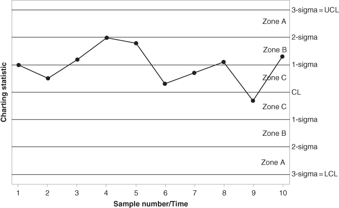
Figure 3.11 Western Electric rule number 4.
Western Electric rule number 1 is illustrated in Figure 3.8 . This rule gives a signal if one or more points plot on or outside the LCL or UCL. The control chart in Figure 3.8 signals at sample number 9. Although this rule is illustrated for a possible upward shift in the process, it also gives a signal if the charting statistics had a perfect mirror‐image copy around the CL, indicating a possible downward shift in the process.
Western Electric rule number 2 is illustrated in Figure 3.9. This rule gives a signal if two of three consecutive points plot outside the 2‐sigma warning limits but still inside the control limits. The control chart in Figure 3.9 signals at sample number 9. Although this rule is illustrated for a possible upward shift in the process, it also gives a signal if the charting statistics had a perfect mirror‐image copy around the CL, indicating a possible downward shift in the process.
Western Electric rule number 3 is illustrated in Figure 3.10. This rule gives a signal if four of five consecutive points plot outside the 1‐sigma warning limits but still inside the control limits. The control chart in Figure 3.10 signals at sample number 10. Although this rule is illustrated for a possible upward shift in the process, it also gives a signal if the charting statistics had a perfect mirror‐image copy around the CL, indicating a possible downward shift in the process.
Western Electric rule number 4 is illustrated in Figure 3.11 . This rule gives a signal if a run of eight consecutive points on one side of the CL occurs. The control chart in Figure 3.11 signals at sample number 8. Although this rule is illustrated for a possible upward shift in the process, it also gives a signal if the charting statistics had a perfect mirror‐image copy around the CL, indicating a possible downward shift in the process.
Some other sensitizing rules have been suggested in the literature and these include:
- Six points in a row steadily increasing or decreasing.
- Fifteen points in a row in Zone C (both above and below the CL); see Figures 3.8 –3.11 for an illustration of the different zones.
- Fourteen points in a row alternatively up and down.
- Eight points in a row on both sides of the CL with none in Zone C; see Figures 3.8 –3.11 for an illustration of the different zones.
- An unusual or non‐random pattern in the data.
- One or more points near a warning or control limit.
In Table 3.8, we list some possible causes of control chart signals.
Table 3.8 Possible causes of control chart signals.
| Signal | Possible Cause |
| One point outside the control limits followed by no anomalous patterns |
Measurement of recording error Isolated/temporary event such as substitute staff |
| Fifteen points in a row in Zone C (both above and below the CL); see Figures 3.8 –3.11 for an illustration of the different zones | Data have been manipulated, i.e., extreme values are not being recorded or are being recorded incorrectly |
| Trends, e.g., six points in a row steadily increasing or decreasing | The gradual drifting of data can indicate wear and tear on measuring equipment or on machinery. It may also result from machine warm‐up and cool‐down or inadequate maintenance |
| Cyclical pattern; see Figure 2.3 |
This may result from environmental changes such as changes in temperature It can also be a result of operator fatigue, or fluctuation in voltage or pressure or some other variable in the machinery Chemical properties of raw material can also play a role |
| Stratification; see Figure 2.4 |
Stratification may result from the incorrect calculation of control limits or from incorrect subgrouping It may also be a result of not recalculating the control limits after process improvement |
| A sudden jump | This could be a result of damaged equipment, new staff, etc. |
3.5.2 Runs‐type Signaling Rules
Runs‐type signaling rules are used to improve the Shewhart chart's sensitivity for detecting smaller process shifts, along with preserving the simplicity of the Shewhart charts. These are also called supplementary rules as they are used to supplement an original chart to make it more sensitive to detecting process changes. The original Shewhart chart uses the charting statistic from the current sample to check if there is a signal or not in order to determine the state of the process; thus, this chart is also known as the 1‐of‐1 chart (based on the 1‐of‐1 rule). While this is reasonable, it might be worthwhile to consider the charting statistics from a few of the previous samples to see if there is a pattern in the signals. For example, if we have signals from two back to back samples (a run of two), a stronger evidence of change would emerge. Charts using such signaling rules are called runs‐rules enhanced charts. Two of the popular signaling rules are the 2‐of‐2 and 2‐of‐3 runs‐type signaling rules and these runs‐rules enhanced charts are labeled the 2‐of‐2 and 2‐of‐3 charts.
Note that the k‐of‐k ![]() runs‐type signaling rule is the general case of the 2‐of‐2 runs‐type signaling rule. The k‐of‐k runs‐type signaling rule signals where k consecutive charting statistics all plot on or outside the control limit(s). A generalization of the k‐of‐k runs‐type signaling rule is the k‐of‐w
runs‐type signaling rule is the general case of the 2‐of‐2 runs‐type signaling rule. The k‐of‐k runs‐type signaling rule signals where k consecutive charting statistics all plot on or outside the control limit(s). A generalization of the k‐of‐k runs‐type signaling rule is the k‐of‐w ![]() runs‐type signaling rule, which signals where k of the last w charting statistics plots on or outside the control limit(s).
runs‐type signaling rule, which signals where k of the last w charting statistics plots on or outside the control limit(s).
While the runs‐rules enhanced charts can make the Shewhart chart more sensitive to a change, there may be some potential costs. The FAR may be increased and the resulting chart might lack the ability to immediately detect a large process shift. The 2‐of‐3 signaling rules, for example, require at least the last two or three charting statistics to signal, which may be potentially costly to the practitioner since the chart's ability to detect a large shift in the process is delayed until at least three samples are collected. Thus, the cost and the benefit need to be carefully weighed before one decides to use a supplementary runs‐rules enhanced chart.
Many parametric control charts with runs‐type signaling rules have been proposed in the literature. The interested reader can take a look at, for example, Roberts (1958), Champ and Woodall (1987), Champ (1992), Klein (2000), Shmueli and Cohen (2003), Acosta‐Mejia (2007), Khoo and Ariffin (2006), Lim and Cho (2009), Cheng and Chen (2011), Santiago and Smith (2013) and others. However, the focus of our discussion is on nonparametric control charts and, accordingly, we focus on nonparametric control charts to monitor location and/or scale with runs‐type signaling rules. Overall, to learn about the advantages and disadvantages of Shewhart‐type control charts supplemented by runs‐type signaling rules, refer to Nelson (1985). Koutras et al. (2007) show that the overall probability of a false alarm when h decision rules are used is

provided that all ![]() decision rules are independent, with rule
decision rules are independent, with rule ![]() having probability
having probability ![]() such that the charting statistic plots on or outside the control limits when the process is IC. Note that Equation 3.16 is not valid in the case of the typical runs‐rules; see Nelson (1985) and Montgomery (2009).
such that the charting statistic plots on or outside the control limits when the process is IC. Note that Equation 3.16 is not valid in the case of the typical runs‐rules; see Nelson (1985) and Montgomery (2009).
3.5.2.1 Signaling Indicators
Let the charting statistic for the ![]() subgroup be denoted by
subgroup be denoted by ![]() for
for ![]() 1, 2, 3, … Let the indicator functions for the one‐sided control charts be denoted by
1, 2, 3, … Let the indicator functions for the one‐sided control charts be denoted by

and

respectively. Thus, ![]() equals 1 and indicates a signal for an upper one‐sided chart when
equals 1 and indicates a signal for an upper one‐sided chart when ![]() plots on or above the UCL. Similarly,
plots on or above the UCL. Similarly, ![]() takes a value 1 and indicates a signal for a lower one‐sided chart when
takes a value 1 and indicates a signal for a lower one‐sided chart when ![]() plots on or below the LCL. Thus, these binary variables are called signaling indicators. For a two‐sided control chart, the signaling indicator may be denoted by
plots on or below the LCL. Thus, these binary variables are called signaling indicators. For a two‐sided control chart, the signaling indicator may be denoted by

so that ![]() indicates whether the charting statistic of
indicates whether the charting statistic of ![]() plots on or above the UCL (
plots on or above the UCL (![]() ), between the two limits (
), between the two limits (![]() ), or on or below the LCL (
), or on or below the LCL (![]() ). The values 1 and 2 indicate that there is a signal, on the high or the low side, respectively, whereas the value 0 indicates there is not a signal and that the process is IC.
). The values 1 and 2 indicate that there is a signal, on the high or the low side, respectively, whereas the value 0 indicates there is not a signal and that the process is IC.
3.5.2.1.1 The 1‐of‐1 Runs‐type Signaling Rule
The most commonly used and least complex charts are the usual Shewhart charts, called 1‐of‐1 charts, which are not supplemented by any runs‐rules. However, they are known to be insensitive in detecting small process shifts. These charts signal when the event ![]() or
or ![]() , or
, or ![]() occurs, respectively, where
occurs, respectively, where
- The 1‐of‐1 runs‐type signaling rule for an upper one‐sided chart:
 .
. - The 1‐of‐1 runs‐type signaling rule for a lower one‐sided chart:
 .
. - The 1‐of‐1 runs‐type signaling rule for a two‐sided chart:
 .
.
Figure 3.12 illustrates points (i) and (ii) of the 1‐of‐1 runs‐type signaling rule for an upper one‐sided and a lower one‐sided chart, respectively. Panel (a) detects an upward shift at time i = 7 when ![]() plots above the UCL, whereas Panel (b) detects a downward shift at time i = 7 when
plots above the UCL, whereas Panel (b) detects a downward shift at time i = 7 when ![]() plots below the LCL. For each chart the process is declared OOC and a search for assignable causes can be started.
plots below the LCL. For each chart the process is declared OOC and a search for assignable causes can be started.

Figure 3.12 The 1‐of‐1 runs‐type signaling rule for an upper one‐sided and a lower one‐sided chart.
Figure 3.13 illustrates point (3) of the 1‐of‐1 runs‐type signaling rule for a two‐sided chart. Both charts signal at time i = 7; at first an upward shift is detected when ![]() plots above the UCL, and then a downward shift is detected when
plots above the UCL, and then a downward shift is detected when ![]() plots below the LCL.
plots below the LCL.

Figure 3.13 The 1‐of‐1 runs‐type signaling rule for a two‐sided chart.
3.5.2.1.2 The k‐of‐k and k‐of‐w Runs‐type Signaling Rules
Several runs‐type signaling rules, such as the 2‐of‐2 and 2‐of‐3 runs‐rules, have been investigated by many authors and proved that their “runs‐rules enhanced” charts outperform the 1‐of‐1 chart.
One‐sided k‐of‐k and k‐of‐w Runs‐type Signaling Rules
To illustrate, we start with the 2‐of‐2 runs‐type signaling rule. This rule uses the last two charting statistics, ![]() and
and ![]() , to determine whether the process is IC or OOC. For the 2‐of‐2 runs‐type signaling rule, an upper one‐sided chart signals when event
, to determine whether the process is IC or OOC. For the 2‐of‐2 runs‐type signaling rule, an upper one‐sided chart signals when event ![]() occurs and a lower one‐sided chart signals when event
occurs and a lower one‐sided chart signals when event ![]() occurs where
occurs where
- an upper one‐sided chart supplemented by a 2‐of‐2 runs‐type signaling rule:

- a lower one‐sided chart supplemented by a 2‐of‐2 runs‐type signaling rule:
 .
.
Panels (a) and (b) in Figure 3.14 illustrate these signaling events ![]() and
and ![]() , and both signal at time i = 7 where two consecutive points plots above (below) the UCL (LCL). For each chart, the process is declared OOC and a search for assignable causes can be started.
, and both signal at time i = 7 where two consecutive points plots above (below) the UCL (LCL). For each chart, the process is declared OOC and a search for assignable causes can be started.

Figure 3.14 The 2‐of‐2 runs‐type signaling rule for an upper one‐sided and a lower one‐sided chart.
Next, we illustrate the 2‐of‐3 runs‐type signaling rule for an upper one‐sided chart and a lower one‐sided chart, respectively. These charts use two of the last three charting statistics ![]() ,
, ![]() , and
, and ![]() to determine whether the process is IC or OOC. Although there are three ways that two of the three charting statistics can result in a signal, only on two of these possibilities does the last charting statistic plot on or above (below) the upper (lower) control limits. The one‐sided charts supplemented by the 2‐of‐3 runs‐type signaling rule signal when event
to determine whether the process is IC or OOC. Although there are three ways that two of the three charting statistics can result in a signal, only on two of these possibilities does the last charting statistic plot on or above (below) the upper (lower) control limits. The one‐sided charts supplemented by the 2‐of‐3 runs‐type signaling rule signal when event ![]() or
or ![]() =
= ![]() occurs where:
occurs where:
| An upper one‐sided chart supplemented by the 2‐of‐3 runs‐type signaling rule |
|
(1) (2) |
| A lower one‐sided chart supplemented by the 2‐of‐3 runs‐type signaling rule |
|
(3) (4) |
Figure 3.15 illustrates these signaling events ![]() ,
, ![]() ,
, ![]() , and
, and ![]() of an upper one‐sided chart and a lower one‐sided chart supplemented by the 2‐of‐3 runs‐type signaling rule, respectively. The upper one‐sided charts in Panel (a) signal at time i = 7 where two of the last three points plot above the UCL. For each chart, the process is declared OOC and a search for assignable causes can be started. Likewise, the lower one‐sided charts in Panel (b) signal at time i = 7 where two of the last three points plot below the LCL. For each chart, the process is declared OOC and a search for assignable causes can be started.
of an upper one‐sided chart and a lower one‐sided chart supplemented by the 2‐of‐3 runs‐type signaling rule, respectively. The upper one‐sided charts in Panel (a) signal at time i = 7 where two of the last three points plot above the UCL. For each chart, the process is declared OOC and a search for assignable causes can be started. Likewise, the lower one‐sided charts in Panel (b) signal at time i = 7 where two of the last three points plot below the LCL. For each chart, the process is declared OOC and a search for assignable causes can be started.
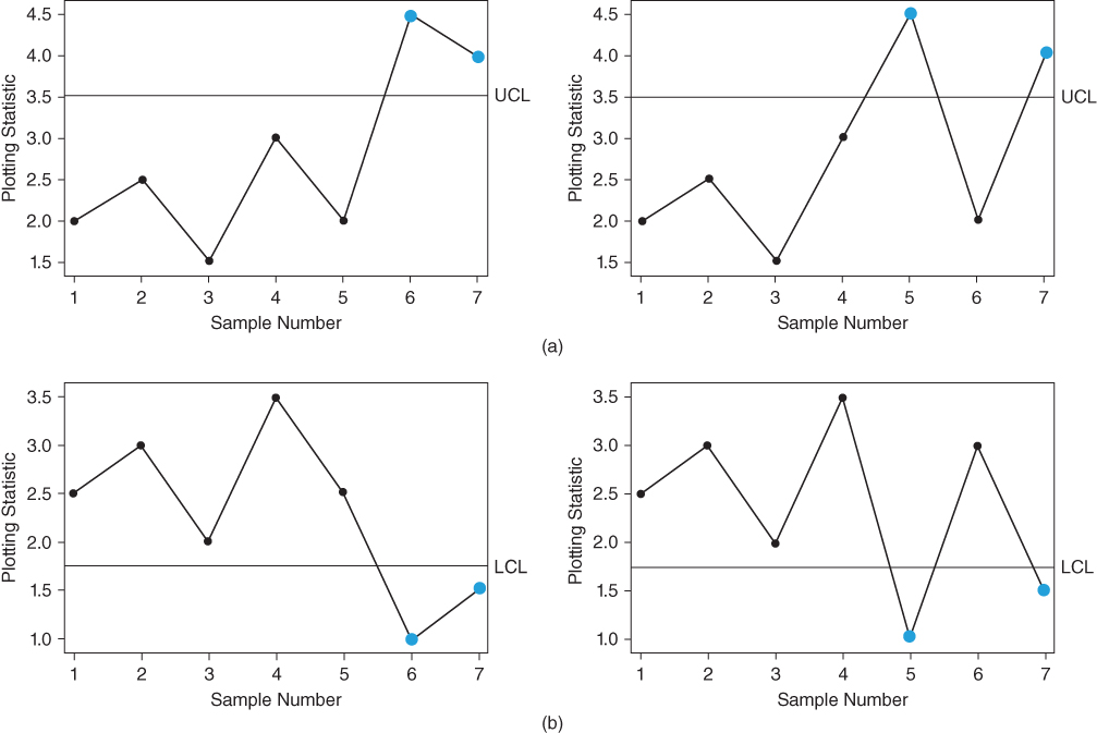
Figure 3.15 The 2‐of‐3 runs‐type signaling rule for an upper one‐sided chart and a lower one‐sided chart.
Some of the patterns of the 2‐of‐3 runs‐type signaling rules are excluded. If the first and the second charting statistics plot outside the control limits, but the third (or last) charting statistic plots between the control limits, the process cannot be declared OOC, because the process has shifted back to being IC and, accordingly, these patterns are excluded from the 2‐of‐3 runs‐type signaling rules. Refer to Figure 3.16, where the upper one‐sided chart supplemented by the 2‐of‐3 runs‐type signaling rule and the lower one‐sided chart supplemented by the 2‐of‐3 runs‐type signaling rule are excluded as signaling events.

Figure 3.16 The 2‐of‐3 runs‐type signaling rules that are excluded for an upper one‐sided and a lower one‐sided chart.
Two‐sided Charts Supplemented by k‐of‐k and k‐of‐w Runs‐type Signaling Rules
A two‐sided chart has both an upper and a lower control limit, thus it can detect either an upward or a downward shift. To illustrate, we start with the 2‐of‐2 runs‐type signaling rule. A two‐sided chart supplemented by a 2‐of‐2 runs‐type signaling rule is much the same as that of the one‐sided charts in the sense that it uses the last two charting statistics, ![]() and
and ![]() , to determine whether the process is IC or OOC, but it is able to detect both an upward or a downward shift. A two‐sided chart supplemented by the 2‐of‐2 runs‐type signaling rule signals when event
, to determine whether the process is IC or OOC, but it is able to detect both an upward or a downward shift. A two‐sided chart supplemented by the 2‐of‐2 runs‐type signaling rule signals when event ![]() or
or ![]() occurs where
occurs where
- both charting statistics plot on or above the UCL:

- both charting statistics plot on or below the LCL:

- the first charting statistic plots on or above the UCL and the second plots on or below the LCL:

- the first charting statistic plots on or below the LCL and the second plots on or above the UCL:
 .
.
Figure 3.17 illustrates these signaling events ![]() ,
, ![]() ,
, ![]() , and
, and ![]() for the two‐sided chart supplemented by 2‐of‐2 runs‐type signaling rules, respectively. Panels (a) and (b) illustrate events
for the two‐sided chart supplemented by 2‐of‐2 runs‐type signaling rules, respectively. Panels (a) and (b) illustrate events ![]() and
and ![]() ; both charts signal at time i = 7, where two consecutive points plots above (below) the UCL (LCL). Panels (c) and (d) illustrate events
; both charts signal at time i = 7, where two consecutive points plots above (below) the UCL (LCL). Panels (c) and (d) illustrate events ![]() and
and ![]() when an upward shift is immediately followed by a downward shift, or vice versa.
when an upward shift is immediately followed by a downward shift, or vice versa.

Figure 3.17 The 2‐of‐2 runs‐type signaling rule for a two‐sided chart.
Next, we illustrate a two‐sided chart with 2‐of‐3 runs‐type signaling rules. Similar to one‐sided chart, a two‐sided chart uses two of the last three charting statistics, ![]() ,
, ![]() , and
, and ![]() , to determine whether the process is IC or OOC. There are up to 12 scenarios where exactly two of the three charting statistics can plot outside the control limits; however, we will only focus on four signaling events
, to determine whether the process is IC or OOC. There are up to 12 scenarios where exactly two of the three charting statistics can plot outside the control limits; however, we will only focus on four signaling events ![]() or
or ![]() that may occur where:
that may occur where:
| Two of the three charting statistics plot on or above the UCL |
|
(1) (2) |
| Two of the three charting statistics plot on or below the LCL |
|
(3) (4) |
Figure 3.18 illustrates these signaling events ![]() ,
, ![]() ,
, ![]() , and
, and ![]() for a two‐sided chart supplemented by 2‐of‐3 runs‐type signaling rules. Panel (a) illustrates events
for a two‐sided chart supplemented by 2‐of‐3 runs‐type signaling rules. Panel (a) illustrates events ![]() and
and ![]() , where exactly two out of the three charting statistics plot on or above the UCL, whereas Panel (b) illustrates events
, where exactly two out of the three charting statistics plot on or above the UCL, whereas Panel (b) illustrates events ![]() and
and ![]() , where exactly two out of the three charting statistics plot on or below the LCL.
, where exactly two out of the three charting statistics plot on or below the LCL.

Figure 3.18 The 2‐of‐3 runs‐type signaling rule for a two‐sided chart.
Figure 3.19 illustrates eight of the 12 scenarios that are excluded as signaling events. Panel (a) shows a possible swing detected, whereas Panel (b) illustrates a downward or upward trend in the process. As mentioned in Figure 3.16 , the four events illustrated in Panel (c) will be excluded as signaling events due to the fact that the last point plots between the control limits; therefore, the process cannot be declared OOC, because the process has shifted back to being IC.

Figure 3.19 The 2‐of‐3 runs‐type signaling rules that are excluded for a two‐sided chart.
3.6 Run‐length Distribution in the Specified Parameter Case (Case K)
The performance of a control chart is analyzed via the run‐length distribution and associated characteristics such as the various moments and percentiles. We discuss the methods of calculating the run‐length distribution of control charts in this section. The discussion is general and applies to all types of control charts, including parametric and nonparametric control charts and the parameter known (Case K) and unknown (Case U) cases. We deal with Case K first.
3.6.1 Methods of Calculating the Run‐length Distribution
There are four methods to calculate (or at least approximate) the run‐length distribution of a control chart. Specifically, in Case K, these are
- the exact approach (for Shewhart and some Shewhart‐type charts);
- the Markov chain (MC) approach;
- the integral equation approach; and
- the computer simulations (the Monte Carlo) approach.
A discussion on each method follows. We consider first the case of Shewhart charts.
3.6.1.1 The Exact Approach (for Shewhart and some Shewhart‐type Charts)
For the Shewhart and some Shewhart‐type control charts, it is easy to calculate the characteristics of the run‐length distribution exactly in Case K. For the two‐sided 3‐sigma Shewhart ![]() chart, the run‐length, which is the number of samples until the first signal, follows a geometric distribution with probability
chart, the run‐length, which is the number of samples until the first signal, follows a geometric distribution with probability ![]() , which equals the FAR, denoted
, which equals the FAR, denoted ![]() , when the process is IC. We provide more details on this later. Thus, in Case K, all IC properties of the Shewhart
, when the process is IC. We provide more details on this later. Thus, in Case K, all IC properties of the Shewhart ![]() control chart can be characterized in terms of the FAR,
control chart can be characterized in terms of the FAR, ![]() , and obtained from the properties of the geometric distribution. Thus, for example, the IC ARL equals
, and obtained from the properties of the geometric distribution. Thus, for example, the IC ARL equals ![]() , the IC SDRL equals
, the IC SDRL equals ![]() , and so on. Figure 3.20 has a display of the run‐length distribution for
, and so on. Figure 3.20 has a display of the run‐length distribution for ![]() . The right‐skewed nature of the distribution is obvious. For smaller values of
. The right‐skewed nature of the distribution is obvious. For smaller values of ![]() , such as 0.0027, which is fairly typical in the industry, the run‐length distribution is even more right‐skewed with an even longer right tail.
, such as 0.0027, which is fairly typical in the industry, the run‐length distribution is even more right‐skewed with an even longer right tail.

Figure 3.20 Run‐length distribution of a Shewhart control chart for the mean in Case K with  .
.
For some well‐known control charts like the CUSUM, the EWMA, and the Shewhart charts with runs‐rules, a more common approach to determining the run‐length distribution has been the clever application of the idea of a Markov chain (MC). The MC theory is more commonly used in the area of stochastic processes and the control charting literature has borrowed some important results from this literature. We describe some of the concepts and the key results below.
3.6.1.2 The Markov Chain Approach
Some theory and concepts in the area of what is called a finite homogeneous MC have been applied to derive the run‐length distribution and various characteristics of the run‐length distribution of some time‐weighted charts, such as the CUSUM and the EWMA. The reader can look up, for example, Fu and Lou (2003) and Balakrishnan and Koutras (2002) for a more detailed treatment of the topics; however, most existing SPC books don't seem to treat this important topic. In this section, some of the basic terminologies, definitions, results, and theorems are provided that give the necessary background for calculating the run‐length distribution of some control charts via the MC approach. These theorems and results are critical to the following chapters; illustrations are provided.
The MC approach entails that the charting statistic is viewed as following a MC (as a stochastic process), with a state space S and a transition probability matrix ![]() . The state space consists of two types of states:
. The state space consists of two types of states:
- one absorbing state (i.e., this state is entered when the chart signals, i.e., when the charting statistic is greater than or equal to the UCL, or less than or equal to the LCL for a two‐sided chart); and
 transient or non‐absorbing states, so that there are
  + 1 states in total.
The (![]() + 1)
+ 1) ![]() (
(![]() + 1) transition probability matrix,
+ 1) transition probability matrix, ![]() , is often written in a partitioned form
, is often written in a partitioned form

where the sub‐matrix ![]() contains all the probabilities of going from one transient state to another and is called the essential transition probability matrix. The column vector
contains all the probabilities of going from one transient state to another and is called the essential transition probability matrix. The column vector ![]() contains all the probabilities of going from each transient state to the absorbing state;
contains all the probabilities of going from each transient state to the absorbing state; ![]() is a row vector of zeros, consisting of the probabilities of going from the absorbing state to each transient state (which are all zero), and the scalar value 1 is the probability of staying in the absorbing state once it has been entered. Note that the key component in using the MC approach is to obtain the essential transition probability matrix
is a row vector of zeros, consisting of the probabilities of going from the absorbing state to each transient state (which are all zero), and the scalar value 1 is the probability of staying in the absorbing state once it has been entered. Note that the key component in using the MC approach is to obtain the essential transition probability matrix ![]() .
.
In the context of MCs, the run‐length random variable N of a control chart is viewed as the waiting time for the MC to enter the absorbing state for the first time. Using this analogy, and assuming that the process starts IC when the chart is implemented, the probability mass function (pmf), the expected value (ARL), the standard deviation (SDRL), and the cdf of N are given by (see Fu and Lou, 2003, Chapter 5)
respectively, where ![]() is the identity matrix,
is the identity matrix, ![]() is the essential transition probability matrix,
is the essential transition probability matrix, ![]() is a column vector with all elements equal to one, and
is a column vector with all elements equal to one, and ![]() is a row vector called the initial probability vector, which contains the probabilities that the MC starts in a given state. The vector
is a row vector called the initial probability vector, which contains the probabilities that the MC starts in a given state. The vector ![]() is typically chosen such that
is typically chosen such that ![]() .
.
The zero‐state and steady‐state modes of analysis are used to characterize the short‐ and long‐term run‐length properties of a control chart, respectively. That is, the zero‐state run‐length is the number of charting statistics plotted before a signal is given when the process begins in some initial state; however, the steady‐state run‐length is the number of charting statistics plotted before a signal is given when the process begins and stays IC for a very long time. Then, at some random time, an OOC signal is observed; see, for example, Champ (1992) and Machado and Costa (2014a, b). Let ![]() denote the row vector of initial probabilities associated with the zero‐state mode, that is
denote the row vector of initial probabilities associated with the zero‐state mode, that is
so that the initial state element on the transition probability matrix corresponds to the value of 1 in Equation 3.25. It should be noted that the 1 is in the middle of the row vector so that the process starts IC. This is done by forcing the initial state to be as close to the CL as possible, that is, the selection of the middle value corresponding to the middle discretized subinterval which, in turn, is the closest one can start to the CL. In the steady‐state, the vector ![]() is replaced by a vector
is replaced by a vector ![]() , that is, the steady‐state initial probability vector. This is given by
, that is, the steady‐state initial probability vector. This is given by
where the elements in Equation 3.26 sum to unity. For example, for ![]() , the
, the ![]() may be equal to
may be equal to ![]() . This would indicate that one would start closer to the CL with the highest probability of 0.3, or one would start further away from the CL with smaller probability 0.2, and, finally, one could start close to the control limits with the smallest probability of 0.15. The smallest probability is assigned to starting close to the UCL and close to the LCL, respectively, because this is not ideal. Another example could be, for
. This would indicate that one would start closer to the CL with the highest probability of 0.3, or one would start further away from the CL with smaller probability 0.2, and, finally, one could start close to the control limits with the smallest probability of 0.15. The smallest probability is assigned to starting close to the UCL and close to the LCL, respectively, because this is not ideal. Another example could be, for ![]() we have
we have ![]() . In this example, we have some elements in
. In this example, we have some elements in ![]() that equal zero and other elements that are non‐zero. Here, it indicates that one would start closer to the CL with the highest probability of 0.8, or one would start further away from the CL with smaller probability 0.1, and, finally, one could start close to the control limits with zero probability.
that equal zero and other elements that are non‐zero. Here, it indicates that one would start closer to the CL with the highest probability of 0.8, or one would start further away from the CL with smaller probability 0.1, and, finally, one could start close to the control limits with zero probability.
From Equation 3.24, it is clear that in order to apply the MC approach to find the run‐length distribution for a given control chart one needs to specify the essential transition probability matrix ![]() . Once the
. Once the ![]() matrix is found, the run‐length distribution and associated characteristics can be obtained easily using the formulas given above for a given initial probability vector. Now, in order to calculate the elements of
matrix is found, the run‐length distribution and associated characteristics can be obtained easily using the formulas given above for a given initial probability vector. Now, in order to calculate the elements of ![]() , the state space first needs to be identified. For an attributes control chart with a discrete charting statistic this is easy, since the number of states will be fixed. However, for a variables control chart, which uses a charting statistic with a continuous distribution, the states of the process thus need to be defined carefully. The steps of how this is typically done are provided below.
, the state space first needs to be identified. For an attributes control chart with a discrete charting statistic this is easy, since the number of states will be fixed. However, for a variables control chart, which uses a charting statistic with a continuous distribution, the states of the process thus need to be defined carefully. The steps of how this is typically done are provided below.
It should be noted that, with runs‐type signaling rules, the number of states is defined by the type of rule used, for example, whether one uses a 2‐of‐2 or a 2‐of‐3 runs‐rules. There is no need to discretize the interval between the LCL and the UCL into ![]() = 2
= 2![]() + 1 subintervals (as explained in Step 1 below), since, as stated before, for runs‐type signaling rules the number of states depends on the type of rule. Also, it should be noted that, with CUSUM charts, the number of states is a fixed number (see Example 3.6). There is no need to discretize the interval between the LCL and the UCL into
+ 1 subintervals (as explained in Step 1 below), since, as stated before, for runs‐type signaling rules the number of states depends on the type of rule. Also, it should be noted that, with CUSUM charts, the number of states is a fixed number (see Example 3.6). There is no need to discretize the interval between the LCL and the UCL into ![]() = 2
= 2![]() + 1 subintervals (as explained in Step 1 below), since, as stated before, for CUSUM charts the number of states will be a fixed number. The steps below apply to the EWMA charts.
+ 1 subintervals (as explained in Step 1 below), since, as stated before, for CUSUM charts the number of states will be a fixed number. The steps below apply to the EWMA charts.
- Step 1: Divide the interval between the LCL and the UCL into
 = 2
= 2 + 1 subintervals of width 2
 = (UCL – LCL)/
 (see Figure 3.21), where each subinterval corresponds to a transient (or an accessible) state of the MC. State
  is said to be accessible from state
  if, and only if, starting in state
  , it is possible that the process will at some stage enter state
  . Note that 2
 = (UCL – LCL)/
 will equal 2
 = 2UCL/
 so that
  = UCL/
 if the control limits are symmetrically placed around zero (i.e., – LCL = UCL). It should be noted that taking larger values of
  would result in more accurate answers. A detailed discussion on the choice of
  is given in Note 3.2.
 - Step 2: Choose the number of discretized subintervals
 to be an odd positive integer so that there is a unique middle entry.
 - Step 3: Declare the charting statistic,
 , to be in the transient state
  at time
  if
if  for
for  and
and  for
for  , where
  denotes the midpoint of the
  th interval.
 - Step 4: Calculate the one‐step transition probabilities (
 's) where
  denotes the probability of moving from state
  to state
  in one step at any point in time.
 - Step 5: Construct the transition probability matrix, consisting of the one‐step transition probabilities, to find the run‐length distribution.
Note that the midpoints (defined in Step 3) can be found using the following general calculation formula
since we assume (for simplicity) that – LCL = UCL. The charting statistic is said to be in the absorbing or OOC state (i.e., ![]() ) if
) if ![]() falls on or outside the control limits. This region is considered absorbing since the process is stopped when a signal is given by the chart. Hence, the process is declared to be OOC whenever
falls on or outside the control limits. This region is considered absorbing since the process is stopped when a signal is given by the chart. Hence, the process is declared to be OOC whenever ![]() is in the absorbing state, whereas the process is considered IC whenever
is in the absorbing state, whereas the process is considered IC whenever ![]() is in a transient state (also referred to as an IC state). Therefore, the IC region consists of v non‐absorbing states, whereas the OOC region is treated as a single absorbing state.
is in a transient state (also referred to as an IC state). Therefore, the IC region consists of v non‐absorbing states, whereas the OOC region is treated as a single absorbing state.

Figure 3.21 Partitioning of the interval between the LCL and the UCL into  = 2
= 2 + 1 subintervals.
As explained before, in order to apply the MC approach, we need expressions for the signaling probabilities so that we can set up the transition probability matrix. The elements of the essential transition probability matrix ![]() are called the one‐step transition probabilities;
are called the one‐step transition probabilities; ![]() for
for ![]() . In order to calculate these probabilities once the states have been defined or identified, we assume that the charting statistic is equal to the midpoint
. In order to calculate these probabilities once the states have been defined or identified, we assume that the charting statistic is equal to the midpoint ![]() whenever it is in state
whenever it is in state ![]() . This is an approximation that becomes more accurate when the numbers of subintervals increase, and is commented on later. For each control chart under consideration, the one‐step transition probabilities are calculated differently. Next, we give another example of using the MC approach to calculate the run‐length distribution of a CUSUM chart.
. This is an approximation that becomes more accurate when the numbers of subintervals increase, and is commented on later. For each control chart under consideration, the one‐step transition probabilities are calculated differently. Next, we give another example of using the MC approach to calculate the run‐length distribution of a CUSUM chart.
3.6.1.3 The Integral Equation Approach
The integral equation approach utilizes mathematics and combinatorics to find a closed form expression of the run‐length distribution. This approach is sometimes challenging in that the expression obtained is typically complex or difficult to evaluate numerically. Often, the exact expression of the run‐length distribution can be found after a considerable amount of work, but here a simulation is done instead, since it is much easier.
3.6.1.4 The Computer Simulations (the Monte Carlo) Approach
Monte Carlo simulations can be used to calculate the characteristics of the run‐length distribution. The popularity of this method stems from the fact that, no matter how complicated the run‐length distribution is, theoretically, computer simulations can almost always be used with relative ease to calculate the run‐length distribution and its associated characteristics fairly accurately, provided that the simulation size is big enough. In this body of work, we use 100 000 simulations since it is well known that the error of a run‐length characteristic can be bounded by increasing the simulation size sufficiently.
The generic steps of a computer simulation procedure to calculate the run‐length distribution for a two‐sided control chart, where the charting statistic is calculated from a random sample, is given as follows. This can be implemented in any software package such as R, SAS, or Matlab.
- Step 1: Specify the necessary parameters, such as the subgroup size, nominal IC average run‐length (or FAR); calculate the control limits.
- Step 2: Assume some process distribution, such as the normal distribution and specify parameters. Generate (simulate) subgroups of random observations from the specified distribution.
- Step 3: Calculate the charting statistic for each subgroup and compare it to the control limits calculated in Step 1.
- Step 4: The number of subgroups needed until the first charting statistic plots on or outside the control limits is recorded as an observation from the run‐length distribution.
- Step 5: Repeat Steps 1 to 4 a total of 100 000 times.
- Step 6: Once we obtain a “data set” with 100 000 observations from the run‐length distribution, the run‐length distribution characteristics of interest, which are descriptive statistics, such as the average, standard deviation, median, percentiles, etc., can be calculated. For example, one can use proc univariate of SAS to find these values. Minitab or R can be used to do the same and graph the boxplots or histograms of the run‐length values for a better understanding of the run‐length distribution.
It may be noted that simulating the run‐length distribution and the associated characteristics may be particularly time consuming in the IC case since the run‐length distribution is heavily right‐skewed, which means that there may be some very large run‐length values, which can take a very long time to be realized. In some cases, one has to be careful that the run‐length characteristic of interest, say, the ARL, is finite, which may not necessarily be the case. A possible shortcut to calculating the run‐length distribution may be to use the explicit expressions to calculate the probability of a signal (and its reciprocal) within the simulations, which may be available for some charts under the assumed process distribution.
3.7 Parameter Estimation Problem and Its Effects on the Control Chart Performance
In the previous sections, we studied the situations where the process is assumed to be normally distributed (or the charting statistic is approximately normally distributed) with parameters that are specified or known. In many practical situations, however, even if normality may be acceptable, the process parameters may not be known and would have to be estimated before process monitoring can start. This situation is referred to as the “standard(s) unknown” or the unknown parameter case and is denoted by Case U. It is well known that ignoring the effects of parameter estimation can be unwise and costly as the run‐length properties of the chart are greatly impacted, which can lead to, for example, many more false alarms than nominally expected (see, for example, Jensen et al., 2006 and Psarakis et al., 2014), which reduces the effectiveness of control charts and increases costs.
Typically, the unknown parameters are estimated using a fixed size reference sample obtained from a Phase I analysis. We discuss the derivation of the run‐length distribution in Case U for the three main types of control charts below. It turns out that the traditional view of the run‐length distribution needs to be re‐examined in light of the correct treatment of parameter estimators used in the control charts (limits).
By the run‐length distribution of a control chart, when parameter estimators are used, one generally refers to what is now known as the unconditional or the marginal run‐length distribution, which is obtained by averaging the run‐length distribution for a given set of estimators over the distribution of these estimators. The run‐length distribution obtained for a given set of estimators is called the conditional run‐length distribution. In the earlier days of SPC, parameter estimates were typically calculated and substituted (plugged‐in) for the parameters, and control limits (and control charts) were set up for prospective (Phase II) monitoring of a process. The effect of parameter estimation was subsumed basically in a mathematical‐statistical step in the derivation of the (unconditional) run‐length distribution. One typically used the run‐length distribution and the associated characteristics (ARL etc.) to characterize chart performance. In recent years, it has been recognized that the plug‐in control charts perform quite differently than their known parameter counterparts, unless a huge number of data were used to calculate the parameter estimates. The amount of data needed can be substantial and may, in fact, be unaffordable or unavailable in a practical situation. While the approach of using the unconditional run‐length distribution and associated properties such as the unconditional ARL may have had merits in providing information about the “average” chart performance, much more practical insight may be provided by the conditional run‐length distribution and its attributes, which help explain the performance of a control chart for the user with the particular parameter estimates for their reference samples. In this context, it is of interest to examine the mean or the expectation of the conditional run‐length distribution, which is the conditional average run‐length, in fact, since the conditional ARL itself is a random variable. However, one also needs to examine other properties, such as the variance of the conditional ARL distribution, to get a better sense of chart performance under parameter estimation. Note that the distinction between the unconditional and the conditional run‐length distribution goes away in the parameter known case when they are both equal to the one and the only run‐length distribution of the control chart.
The overarching theme in all of this is, of course, is the amount of Phase I data that is required for parameter estimation so that predictable chart performance can be assured. It might also be necessary to take another look at measures of chart performance and how to design the control charts (i.e., obtain the correct charting constants) for the amount of data at hand to guarantee such performance.
We now revisit the control charts that were discussed earlier in this chapter for the known parameter case (Case K) and in the case when the parameters are unknown, that is, Case U. Note that we still assume that the underlying process distribution is normal. When the parameters are unknown, they are usually estimated from a retrospective analysis of historical data, often called a Phase I analysis. Control charts play an important role in Phase I analysis; we discuss some Phase I charts in Chapter 5. Once the Phase I analysis is completed, a set of reference data is obtained, which is assumed to be derived from an IC process. These data are used to estimate parameters and the control limits, which are then used prospectively to monitor incoming new or test data. This part of statistical process control is called a Phase II analysis. Thus, in this section, we first illustrate Phase II control charts where unknown process parameters are estimated from Phase I. We also discuss properties of the Case U control charts and illustrate the so‐called conditioning/unconditioning (CUC) method to derive the run‐length distribution and its various attributes, such as the average run‐length. Note that a lot of work has been done in this area recently, yet more work is in progress and further new results and a clearer understanding are expected.
3.8 Parametric Variables Control Charts in Case U
3.8.1 Shewhart Control Charts in Case U
3.8.1.1 Shewhart Control Charts for the Mean in Case U
In our discussion of parametric variables control charts in Case U, we assume that the process follows a normal distribution, but at least one (or both) of the process parameters, the mean and the standard deviation, is (are) unknown. Although other process distributions can be assumed in practice, we discuss the case of the normal distribution to be consistent with the earlier developments in the chapter for the known parameter case (see Section 3.2). Before continuing, we make some finer classifications within Case U. When two parameters are in play, as is the case here, we can have four cases, namely, Case KK (mean known and standard deviation known), which is often referred to as just Case K, Case KU (mean known and standard deviation unknown), Case UK (mean unknown and standard deviation known), and Case UU (both mean and standard deviation unknown). In this section, we consider perhaps the most practical situation, Case UU, when both of these parameters are unknown. So Case U refers to one of the three cases, Case KU, UK or UU. Other situations can be treated in a similar way (see for example, Chakraborti, 2000). In addition, we assume that a reference (Phase I) sample comprising ![]() samples, each of size
samples, each of size ![]() , is available after a successful Phase I analysis to estimate these unknown parameters.
, is available after a successful Phase I analysis to estimate these unknown parameters.
Suppose that ![]() ,
, ![]() , and
, and ![]() denote the
denote the ![]() Phase I sample means and standard deviations, respectively. Also, let
Phase I sample means and standard deviations, respectively. Also, let ![]() denote the
denote the ![]() Phase I sample ranges. The process mean
Phase I sample ranges. The process mean ![]() is typically estimated by the average of the m sample means or the grand mean,
is typically estimated by the average of the m sample means or the grand mean, ![]() . Conversely, several estimators have been proposed to estimate the process standard deviation
. Conversely, several estimators have been proposed to estimate the process standard deviation ![]() . We use some of these estimators to illustrate various points. Letting
. We use some of these estimators to illustrate various points. Letting ![]() denote the chosen Phase I estimator of
denote the chosen Phase I estimator of ![]() , the control limits for the two‐sided Phase II k‐sigma Shewhart
, the control limits for the two‐sided Phase II k‐sigma Shewhart ![]() control chart for the mean in Case UU are given by
control chart for the mean in Case UU are given by

The control limits in Equation 3.13
may be referred to as the plug‐in limits as they are of the same form as in Case K, with estimators of the mean and the standard deviations used in place of the known IC values of the parameters. The choice of the charting constant ![]() is an interesting question. For many years, the value 3 was used in analogy with a 3‐sigma chart in Case K. It is now understood that, with plug‐in limits,
is an interesting question. For many years, the value 3 was used in analogy with a 3‐sigma chart in Case K. It is now understood that, with plug‐in limits, ![]() is not a good choice in that it increases the number of false alarms, unless there is a very large number of Phase I data available, which may be in the hundreds or even in the thousands. In fact, in Case U, the choice of the charting constant depends on
is not a good choice in that it increases the number of false alarms, unless there is a very large number of Phase I data available, which may be in the hundreds or even in the thousands. In fact, in Case U, the choice of the charting constant depends on ![]() , and the given nominal IC average run‐length. In Case K, alternatively, the charting constant depends only on
, and the given nominal IC average run‐length. In Case K, alternatively, the charting constant depends only on ![]() and the nominal IC average run‐length. More details about this are provided later.
and the nominal IC average run‐length. More details about this are provided later.
3.8.1.2 Shewhart Control Charts for the Standard Deviation in Case U
As in Case K, the variation of a process must be monitored to ensure that it remains IC. The Shewhart control limits for the process mean in Case U depend on the process standard deviation. Thus, unless the standard deviation remains IC, the control chart for the mean will not be informative and useful. So, we need to monitor the variance or the standard deviation using a control chart.
As noted earlier, there are several possible estimators ![]() that can be used to monitor the standard deviation
that can be used to monitor the standard deviation ![]() . The popular choices include functions of the sample range (
. The popular choices include functions of the sample range (![]() ), or the sample standard deviation (
), or the sample standard deviation (![]() ), or the sample variance (
), or the sample variance (![]() ). Typically, we use a control chart to monitor the process mean together with a control chart to monitor the process variation. If the variation is IC, we go ahead and examine the control chart for the mean.
). Typically, we use a control chart to monitor the process mean together with a control chart to monitor the process variation. If the variation is IC, we go ahead and examine the control chart for the mean.
A Shewhart ![]() chart for the mean, for example, is often used together with a Shewhart
chart for the mean, for example, is often used together with a Shewhart ![]() chart for the spread. Note that, for illustration purposes, we use the Shewhart
chart for the spread. Note that, for illustration purposes, we use the Shewhart ![]() chart for
chart for ![]() , even though recent literature recommends using a different chart, such as the one based on the standard deviation (see, for instance, Mahmoud et al., 2010 and Epprecht, Loureiro, and Chakraborti, 2016). We do this because the Shewhart
, even though recent literature recommends using a different chart, such as the one based on the standard deviation (see, for instance, Mahmoud et al., 2010 and Epprecht, Loureiro, and Chakraborti, 2016). We do this because the Shewhart ![]() chart is simple and continues to be used in the industry.
chart is simple and continues to be used in the industry.
Let ![]() denote the average range. The CL and the control limits for the Shewhart R control chart for
denote the average range. The CL and the control limits for the Shewhart R control chart for ![]() in the unknown parameter case are given by (see Montgomery, 2009, p. 229)
in the unknown parameter case are given by (see Montgomery, 2009, p. 229)

where

and ![]() and
and ![]() are, respectively, the mean and the standard deviation of a range in a random sample of size n from the standard normal distribution. We provide the formulas here for completeness as these are not available in many textbooks.
are, respectively, the mean and the standard deviation of a range in a random sample of size n from the standard normal distribution. We provide the formulas here for completeness as these are not available in many textbooks.

where ![]() and
and

denotes the pdf of the range of the sample of size n from the standard normal distribution with pdf ![]() and cdf
and cdf ![]() (see, for example, Gibbons and Chakraborti, 2010). The integrals involved in these expressions can be calculated numerically or estimated in a simulation study in order to evaluate the constants
(see, for example, Gibbons and Chakraborti, 2010). The integrals involved in these expressions can be calculated numerically or estimated in a simulation study in order to evaluate the constants ![]() and
and ![]() . They both depend on the sample size
. They both depend on the sample size ![]() and are tabulated in Table C of Appendix A. Note that
and are tabulated in Table C of Appendix A. Note that ![]() is an unbiased estimator of
is an unbiased estimator of ![]() so that
so that ![]() is called an unbiasing constant.
is called an unbiasing constant.
The control limits given in Equation 3.31 are of the same form as in Case K but the values of the charting constants ![]() and
and ![]() are different. However, the control limits in Equations 3.32 are the 3‐sigma limits and have some serious deficiencies, see, for example, Diko et al. (2016), particularly when
are different. However, the control limits in Equations 3.32 are the 3‐sigma limits and have some serious deficiencies, see, for example, Diko et al. (2016), particularly when ![]() is small. We consider some alternatives to the R chart control limits based on probability limits later in this section.
is small. We consider some alternatives to the R chart control limits based on probability limits later in this section.
Using a similar idea, but employing the standard deviation of the sample and not the range, the CL and the control limits for the Shewhart S control chart for ![]() in the unknown parameter case are given by (see Montgomery, 2009, p. 253)
in the unknown parameter case are given by (see Montgomery, 2009, p. 253)

where ![]() is the average standard deviation and the constants are given by
is the average standard deviation and the constants are given by

where ![]() denotes the gamma function with
denotes the gamma function with ![]() ! when
! when ![]() is a positive integer. Note that
is a positive integer. Note that ![]() is also an unbiased estimator of
is also an unbiased estimator of ![]() . The constants
. The constants ![]() and
and ![]() can be easily calculated from the formulas and are tabulated in Table H in Appendix A.
can be easily calculated from the formulas and are tabulated in Table H in Appendix A.
Again, note that these control limits are the 3‐sigma limits and, as in the case of the R charts, also have some deficiencies, particularly when ![]() is small. We also consider some alternatives to the
is small. We also consider some alternatives to the ![]() chart control limits.
chart control limits.
It is well known that the probability limits are more appropriate for the standard deviation since the distribution of the estimator ![]() (used in the charting statistic) is right‐skewed. The skewness is more pronounced when the Phase II sample size
(used in the charting statistic) is right‐skewed. The skewness is more pronounced when the Phase II sample size ![]() is smaller, which is typically the case in SPC. Intuitively, the lower control limit on a chart for
is smaller, which is typically the case in SPC. Intuitively, the lower control limit on a chart for ![]() should be positive (and not zero) so that the control chart is able to detect both increases and decreases in
should be positive (and not zero) so that the control chart is able to detect both increases and decreases in ![]() . The increase in
. The increase in ![]() indicates process degradation and is perhaps more important, but a decrease in
indicates process degradation and is perhaps more important, but a decrease in ![]() can also be meaningful as it indicates possible improvements in the process. However, the standard 3‐sigma limits used in Case K, which are based on the normal approximation to the distribution of
can also be meaningful as it indicates possible improvements in the process. However, the standard 3‐sigma limits used in Case K, which are based on the normal approximation to the distribution of ![]() can lead to a negative LCL, which is then typically reset to 0. This is, indeed, the case for
can lead to a negative LCL, which is then typically reset to 0. This is, indeed, the case for ![]() , which includes the most common subgroup used in practice, namely,
, which includes the most common subgroup used in practice, namely, ![]() . Although the 3‐sigma limits are perhaps more popular due to their simplicity, note that many authors have advocated their use with charting statistics with a skewed distribution. Montgomery (2009, p. 242) mentions the probability limits and cites Grant and Leavenworth (1980) for the constants needed to set up such control limits. However, note that these limits are correct and appropriate in Case K, the known parameter case. These constants need to be adjusted or adapted for the unknown parameter case, which was recently considered in Diko et al. (2016). We present a brief discussion on this important practical problem next.
. Although the 3‐sigma limits are perhaps more popular due to their simplicity, note that many authors have advocated their use with charting statistics with a skewed distribution. Montgomery (2009, p. 242) mentions the probability limits and cites Grant and Leavenworth (1980) for the constants needed to set up such control limits. However, note that these limits are correct and appropriate in Case K, the known parameter case. These constants need to be adjusted or adapted for the unknown parameter case, which was recently considered in Diko et al. (2016). We present a brief discussion on this important practical problem next.
To this end, note that the Phase II probability limits for the ![]() chart (with estimator
chart (with estimator ![]() ) and the
) and the ![]() chart (with estimator
chart (with estimator ![]() ) in Case U are given by
) in Case U are given by

and

respectively, where the charting statistics are the range ![]() and the standard deviation
and the standard deviation ![]() of the ith Phase II sample and the constants
of the ith Phase II sample and the constants ![]() and
and ![]() ,
, ![]() are obtained for given values of
are obtained for given values of ![]() ,
, ![]() and a nominal IC average run‐length value, such as 370. These constants are provided in Table H in Appendix A. Some details about the derivations of these constants are provided in Appendix 3.3. The value
and a nominal IC average run‐length value, such as 370. These constants are provided in Table H in Appendix A. Some details about the derivations of these constants are provided in Appendix 3.3. The value ![]() shown in these tables represents the total tail probability beyond the lower and the upper control limits, under the IC distribution of the charting statistic. This is needed while calculating the probability limits.
shown in these tables represents the total tail probability beyond the lower and the upper control limits, under the IC distribution of the charting statistic. This is needed while calculating the probability limits.
Finally, consider ![]() , as the “pooled” estimator of
, as the “pooled” estimator of ![]() based on averaging the Phase I sample variances. This is the estimator recommended (see, for example, Mahmoud et al., 2010) in the literature because of its superior statistical properties. The CL and the control limits for the Phase II
based on averaging the Phase I sample variances. This is the estimator recommended (see, for example, Mahmoud et al., 2010) in the literature because of its superior statistical properties. The CL and the control limits for the Phase II ![]() chart with
chart with ![]() used as an estimator of
used as an estimator of ![]() in the unknown parameter case can be written as
in the unknown parameter case can be written as

where the charting statistic is ![]() and the constants
and the constants ![]() and
and ![]() are given in Table H in Appendix A for various values of
are given in Table H in Appendix A for various values of ![]() and
and ![]() 5, and 10, and for nominal IC average run‐length values of 370 and 500, respectively. Note that one can also use the unbiased version of
5, and 10, and for nominal IC average run‐length values of 370 and 500, respectively. Note that one can also use the unbiased version of ![]() in the control charts, but it can be seen that the unbiasing constant is approximately equal to one for typical
in the control charts, but it can be seen that the unbiasing constant is approximately equal to one for typical ![]() and
and ![]() values. Again, some details about the derivations of these constants are provided in Appendix 3.3.
values. Again, some details about the derivations of these constants are provided in Appendix 3.3.
3.8.2 CUSUM Chart for the Mean in Case U
In Case U, the charting constants, ![]() and
and ![]() , depend on the factors
, depend on the factors ![]() and are obtained for a given nominal IC average run‐length; see Table 3.20. The choice of the charting constants for the parametric CUSUM chart is not as straightforward as in Case K. This is shown with an example in Section 3.9.
and are obtained for a given nominal IC average run‐length; see Table 3.20. The choice of the charting constants for the parametric CUSUM chart is not as straightforward as in Case K. This is shown with an example in Section 3.9.
3.8.3 EWMA Chart for the Mean in Case U
For the EWMA chart in Case U, the charting constants, λ and ![]() , depend on the factors
, depend on the factors ![]() and are obtained for a given nominal IC average run‐length; see Table 3.23. As in the case of the CUSUM chart, the choice of the charting constants for the parametric EWMA chart is not as straightforward as in Case K. This is illustrated with an example in Section 3.9
.
and are obtained for a given nominal IC average run‐length; see Table 3.23. As in the case of the CUSUM chart, the choice of the charting constants for the parametric EWMA chart is not as straightforward as in Case K. This is illustrated with an example in Section 3.9
.
3.9 Types of Parametric Control Charts in Case U: Illustrative Examples
In this section, we provide some examples of classical parametric, that is, normal theory control charts in Case U.
3.9.1 Charts for the Mean
Table 3.13 Measurements used to construct the Shewhart ![]() control chart.
control chart.
| Sample | (a) | (b) | (c) | (d) | ||||
| 1 | 1.3235 | 1.4128 | 1.6744 | 1.4573 | 1.6914 | 1.5119 | 0.1635 | 0.3679 |
| 2 | 1.4314 | 1.3592 | 1.6075 | 1.4666 | 1.6109 | 1.4951 | 0.1111 | 0.2517 |
| 3 | 1.4284 | 1.4871 | 1.4932 | 1.4324 | 1.5674 | 1.4817 | 0.0565 | 0.1390 |
| 4 | 1.5028 | 1.6352 | 1.3841 | 1.2831 | 1.5507 | 1.4712 | 0.1389 | 0.3521 |
| 5 | 1.5604 | 1.2735 | 1.5265 | 1.4363 | 1.6441 | 1.4882 | 0.1412 | 0.3706 |
| 6 | 1.5955 | 1.5451 | 1.3574 | 1.3281 | 1.4198 | 1.4492 | 0.1168 | 0.2674 |
| 7 | 1.6274 | 1.5064 | 1.8366 | 1.4177 | 1.5144 | 1.5805 | 0.1614 | 0.4189 |
| 8 | 1.4190 | 1.4303 | 1.6637 | 1.6067 | 1.5519 | 1.5343 | 0.1077 | 0.2447 |
| 9 | 1.3884 | 1.7277 | 1.5355 | 1.5176 | 1.3688 | 1.5076 | 0.1439 | 0.3589 |
| 10 | 1.4039 | 1.6697 | 1.5089 | 1.4627 | 1.5220 | 1.5134 | 0.0988 | 0.2658 |
| 11 | 1.4158 | 1.7667 | 1.4278 | 1.5928 | 1.4181 | 1.5242 | 0.1548 | 0.3509 |
| 12 | 1.5821 | 1.3355 | 1.5777 | 1.3908 | 1.7559 | 1.5284 | 0.1682 | 0.4204 |
| 13 | 1.2856 | 1.4106 | 1.4447 | 1.6398 | 1.1928 | 1.3947 | 0.1699 | 0.4470 |
| 14 | 1.4951 | 1.4036 | 1.5893 | 1.6458 | 1.4969 | 1.5261 | 0.0937 | 0.2422 |
| 15 | 1.3589 | 1.2863 | 1.5996 | 1.2497 | 1.5471 | 1.4083 | 0.1568 | 0.3499 |
| 16 | 1.5747 | 1.5301 | 1.5171 | 1.1839 | 1.8662 | 1.5344 | 0.2423 | 0.6823 |
| 17 | 1.3680 | 1.7269 | 1.3957 | 1.5014 | 1.4449 | 1.4874 | 0.1432 | 0.3589 |
| 18 | 1.4163 | 1.3864 | 1.3057 | 1.6210 | 1.5573 | 1.4573 | 0.1289 | 0.3153 |
| 19 | 1.5796 | 1.4185 | 1.6541 | 1.5116 | 1.7247 | 1.5777 | 0.1195 | 0.3062 |
| 20 | 1.7106 | 1.4412 | 1.2361 | 1.3820 | 1.7601 | 1.5060 | 0.2230 | 0.5240 |
| 21 | 1.4371 | 1.5051 | 1.3485 | 1.5670 | 1.4880 | 1.4691 | 0.0819 | 0.2185 |
| 22 | 1.4738 | 1.5936 | 1.6583 | 1.4973 | 1.4720 | 1.5390 | 0.0832 | 0.1863 |
| 23 | 1.5917 | 1.4333 | 1.5551 | 1.5295 | 1.6866 | 1.5592 | 0.0922 | 0.2533 |
| 24 | 1.6399 | 1.5243 | 1.5705 | 1.5563 | 1.5530 | 1.5688 | 0.0431 | 0.1156 |
| 25 | 1.5797 | 1.3663 | 1.6240 | 1.3732 | 1.6887 | 1.5264 | 0.1482 | 0.3224 |
The estimator of the mean ![]() is the mean of the Phase I sample means or the grand mean
is the mean of the Phase I sample means or the grand mean

As noted above, the estimators ![]() used in the control limits are based on either (i) the average of the sample ranges,
used in the control limits are based on either (i) the average of the sample ranges, ![]() or (ii) the average of sample standard deviations,
or (ii) the average of sample standard deviations, ![]() or the pooled estimator
or the pooled estimator ![]() = 0.1391. Note that all three estimators of
= 0.1391. Note that all three estimators of ![]() are close to each other.
are close to each other.
The Phase II control charts for the mean are given below.

The charting constants for the Shewhart chart in Case U are tabulated and shown in Table 3.14. For convenience, the same table is given in Table G among the tables in Appendix A. These are based on the works in Chakraborti (2000, 2006) using the unconditional method. From Table G, it can be seen that the charting constant for m = 25, n = 5 is equal to 2.9725 and 3.0574 for a nominal ARLIC = 370 and 500, respectively. Thus, for example, the Phase II control limits for the mean using the pooled estimator ![]() are given by
are given by ![]() and
and ![]() , respectively.
, respectively.
Table 3.14 Charting constants for the Shewhart ![]() control chart for the mean in Case UU for n = 5, varying m and ARLIC = 370 and 500, respectively, using the unconditional method.
control chart for the mean in Case UU for n = 5, varying m and ARLIC = 370 and 500, respectively, using the unconditional method.
| m | ARLIC = 370 | ARLIC = 500 |
| 5 | 2.7838 | 2.8463 |
| 10 | 2.9083 | 2.9844 |
| 20 | 2.9630 | 3.0465 |
| 25 | 2.9725 | 3.0574 |
| 30 | 2.9784 | 3.0643 |
| 35 | 2.9823 | 3.0690 |
| 40 | 2.9852 | 3.0723 |
| 45 | 2.9873 | 3.0748 |
| 50 | 2.9889 | 3.0768 |
| 75 | 2.9933 | 3.0821 |
| 100 | 2.9952 | 3.0845 |
| 200 | 2.9977 | 3.0877 |
| 300 | 2.9985 | 3.0886 |
It is interesting to examine the entries in Table 3.14
. Clearly, the required charting constant is not equal to its counterpart in Case K unless a large number of Phase I samples is used. For example, for ARLIC = 370, only when ![]() is about 100 or more, for
is about 100 or more, for ![]() , does the charting constant get closer to 3, the value for the 3‐sigma limit, which is appropriate for the known parameter case. Also, note that the unconditional ARLIC driven control limits seem to be slightly narrower than those in Case K.
, does the charting constant get closer to 3, the value for the 3‐sigma limit, which is appropriate for the known parameter case. Also, note that the unconditional ARLIC driven control limits seem to be slightly narrower than those in Case K.
Suppose now that at the end of the Phase I analysis, 10 prospective (Phase II) independent random samples are made available. The sample means are shown in Column (b) of Table 3.15.
Table 3.15 Phase II data for the Shewhart ![]() control chart and charting statistics.
control chart and charting statistics.
| Sample | (a) | (b) | (c) | (d) | ||||
| 1 | 1.4231 | 1.3457 | 1.3211 | 1.4654 | 1.3845 | 1.3880 | 0.5099 | 0.0581 |
| 2 | 1.4213 | 1.4620 | 1.3394 | 1.6338 | 1.1239 | 1.3961 | 0.2970 | 0.1863 |
| 3 | 1.4885 | 1.5635 | 1.5446 | 1.5252 | 1.2665 | 1.4777 | 0.2576 | 0.1213 |
| 4 | 1.4158 | 1.5190 | 1.6259 | 1.3683 | 1.4117 | 1.4681 | 0.2999 | 0.1041 |
| 5 | 1.5129 | 1.3825 | 1.5784 | 1.3347 | 1.2785 | 1.4174 | 0.5099 | 0.1249 |
| 6 | 1.4660 | 1.3371 | 1.5378 | 1.6740 | 1.6637 | 1.5357 | 0.3369 | 0.1413 |
| 7 | 1.7342 | 1.2176 | 1.4747 | 1.6500 | 1.3623 | 1.4878 | 0.5166 | 0.2097 |
| 8 | 1.4146 | 1.2826 | 1.2620 | 1.3767 | 1.4036 | 1.3479 | 0.1526 | 0.0707 |
| 9 | 1.2262 | 1.4307 | 1.4523 | 1.5234 | 1.4574 | 1.4180 | 0.2971 | 0.1127 |
| 10 | 1.4625 | 1.4568 | 1.6827 | 1.4944 | 1.4810 | 1.5155 | 0.2259 | 0.0947 |
Figure 3.24 displays the means of these 10 prospective sample means, ![]() , plotted on a Shewhart
, plotted on a Shewhart ![]() control chart together with both sets of control limits, the 3‐sigma limits, and the adjusted (corrected) limits. This display is typically referred to as a Shewhart
control chart together with both sets of control limits, the 3‐sigma limits, and the adjusted (corrected) limits. This display is typically referred to as a Shewhart ![]() control chart or an “X‐bar” chart.
control chart or an “X‐bar” chart.

Figure 3.24 A Shewhart  control chart for monitoring process mean when both the process mean and standard deviation are unknown.
Note that the estimator of ![]() used in the chart was the pooled estimator
used in the chart was the pooled estimator ![]() . As always, once the control chart is drawn, a decision is to be made about the status of the process. In Figure 3.24
, none of the sample means plots outside the control limits and the points do not seem to exhibit any non‐random pattern. Hence, we conclude that the process is functioning in a state of statistical control with respect to the mean. It is also seen that the two sets of limits are quite close to one another, with the corrected limits being slightly shorter.
. As always, once the control chart is drawn, a decision is to be made about the status of the process. In Figure 3.24
, none of the sample means plots outside the control limits and the points do not seem to exhibit any non‐random pattern. Hence, we conclude that the process is functioning in a state of statistical control with respect to the mean. It is also seen that the two sets of limits are quite close to one another, with the corrected limits being slightly shorter.
3.9.2 Charts for the Standard Deviation
Here we illustrate the R and the S charts which can be used to monitor the spread and the standard deviation, respectively. We start with an example of the Shewhart R chart.
In Figure 3.25 , all of the points plot between the control limits and there are no anomalous patterns in the data. Hence, we conclude that the process is functioning in statistical control with respect to spread. Note that the adjusted control limits are wider in the unknown parameter case, which is expected since additional variation is introduced through the parameter estimates.
In Figure 3.26, all of the points plot between the control limits and there are no anomalous patterns in the data. Hence, we conclude that the process is functioning in statistical control with respect to variation. Again, note that the control limits are wider in the unknown parameter case, which is expected since additional variation is introduced through the parameter estimates.

Figure 3.26 Shewhart S chart with  as estimator for monitoring process standard deviation when parameters are unknown.
3.9.2.1 Using the Estimator Sp
Next, we illustrate the probability limits based Shewhart S chart with ![]() as the estimator of
as the estimator of ![]() . Note that, for this data set, the Phase I estimator
. Note that, for this data set, the Phase I estimator ![]() 0.1391. From Table H in Appendix A, the needed charting constants are found to be
0.1391. From Table H in Appendix A, the needed charting constants are found to be ![]() and
and ![]() for a nominal ARLIC = 370. Thus, the probability limits‐based Shewhart S chart is given by
for a nominal ARLIC = 370. Thus, the probability limits‐based Shewhart S chart is given by ![]() and
and ![]() with
with ![]() . Note that this chart is slightly narrower than the probability limits‐based Shewhart S chart using the estimator
. Note that this chart is slightly narrower than the probability limits‐based Shewhart S chart using the estimator ![]() shown in Figure 3.26
. This is expected since
shown in Figure 3.26
. This is expected since ![]() is a more efficient estimator than
is a more efficient estimator than ![]() .
.
In Figure 3.27, all of the points plot between the control limits and there are no anomalous patterns in the data. Hence, we conclude that the process is functioning in statistical control with respect to variation.

Figure 3.27 Shewhart  chart with
  as estimator for monitoring process standard deviation when parameters are unknown.
Table 3.16 Measurements used to construct the parametric CUSUM control chart for the individual data and the charting statistic.
| (a) | (b) | |
| Period, i | xi | |
| 1 | 9.45 | |
| 2 | 7.99 | 1.46 |
| 3 | 9.29 | 1.30 |
| 4 | 11.66 | 2.37 |
| 5 | 12.16 | 0.50 |
| 6 | 10.18 | 1.98 |
| 7 | 8.04 | 2.14 |
| 8 | 11.46 | 3.42 |
| 9 | 9.20 | 2.26 |
| 10 | 10.34 | 1.14 |
| 11 | 9.03 | 1.31 |
| 12 | 11.47 | 2.44 |
| 13 | 10.51 | 0.96 |
| 14 | 9.40 | 1.11 |
| 15 | 10.08 | 0.68 |
| 16 | 9.37 | 0.71 |
| 17 | 10.62 | 1.25 |
| 18 | 10.31 | 0.31 |
| 19 | 8.52 | 1.79 |
| 20 | 10.84 | 2.32 |
Suppose now that at the end of the Phase I analysis that 10 prospective independent measurements are made available.
Table 3.17 Phase II data for the parametric CUSUM control chart.
| Period, i | xi |
| 1 | 10.90 |
| 2 | 9.33 |
| 3 | 12.29 |
| 4 | 11.50 |
| 5 | 10.60 |
| 6 | 11.08 |
| 7 | 10.38 |
| 8 | 11.62 |
| 9 | 11.31 |
| 10 | 10.52 |
In his Table 3.1
, Hawkins (1993) recommends that, for a shift of about ![]() in the process mean, taking
in the process mean, taking ![]() and
and ![]() so that
so that ![]() and
and ![]() , gives an ARLIC = 370. In doing so, we find the design parameters
, gives an ARLIC = 370. In doing so, we find the design parameters ![]() and
and ![]() , respectively.
, respectively.
We monitor the process mean prospectively in Phase II based on the 10 samples given in Table 3.17. It will be seen from Table 3.18 that the charting constant ![]() for m = 20, n = 1,
for m = 20, n = 1, ![]() = 0.5, and a nominal ARL0 = 370 is equal to 4.1 and not 4.77, as in Case K. At this point, note that the values in Table 3.18
were obtained using simulation, and show the impact of the estimation of parameters on the Phase II control limits. The correct value of
= 0.5, and a nominal ARL0 = 370 is equal to 4.1 and not 4.77, as in Case K. At this point, note that the values in Table 3.18
were obtained using simulation, and show the impact of the estimation of parameters on the Phase II control limits. The correct value of ![]() is thus
is thus ![]() . For larger values of
. For larger values of ![]() , around 100, the
, around 100, the ![]() values seem to converge to their values in Case K.
values seem to converge to their values in Case K.
Table 3.18 The charting constant h for the parametric (Normal Theory) CUSUM control chart for the mean in Case UU for n =1, k = 0.5, varying m and ARLIC = 370 and 500.
| m | ARLIC = 370 | ARLIC = 500 |
| 20 | 4.100 | 4.300 |
| 25 | 4.390 | 4.603 |
| 50 | 4.470 | 4.980 |
| 75 | 4.476 | 5.132 |
| 100 | 4.476 | 5.132 |
| 125 | 4.770 | 5.132 |
| 150 | 4.770 | 5.132 |
| 200 | 4.770 | 5.132 |
| 250 | 4.770 | 5.132 |
| 300 | 4.770 | 5.132 |
| 500 | 4.770 | 5.132 |
| 1000 | 4.770 | 5.120 |
The CUSUM charting statistics, ![]() and
and ![]() , are shown in Columns (b) and (d) of Table 3.19, respectively, whereas the corresponding quantities,
, are shown in Columns (b) and (d) of Table 3.19, respectively, whereas the corresponding quantities, ![]() and
and ![]() , are given in Columns (c) and (e), respectively. To illustrate the calculations, consider period 1. The charting statistics are calculated as in the parameter known case, except that we use
, are given in Columns (c) and (e), respectively. To illustrate the calculations, consider period 1. The charting statistics are calculated as in the parameter known case, except that we use ![]() for
for ![]() . Thus,
. Thus,

and

Table 3.19 Phase II data for the parametric CUSUM control chart.
| (a) | (b) | (c) | (d) | (e) | |
| Period, i | xi | ||||
| 0 | 0 | ||||
| 1 | 10.90 | 0.217 | 1 | 0 | 0 |
| 2 | 9.33 | 0.000 | 2 | 0 | 0 |
| 3 | 12.29 | 1.607 | 3 | 0 | 0 |
| 4 | 11.50 | 2.424 | 4 | 0 | 0 |
| 5 | 10.60 | 2.341 | 5 | 0 | 0 |
| 6 | 11.08 | 2.738 | 6 | 0 | 0 |
| 7 | 10.38 | 2.435 | 7 | 0 | 0 |
| 8 | 11.62 | 3.372 | 8 | 0 | 0 |
| 9 | 11.31 | 3.999 | 9 | 0 | 0 |
| 10 | 10.52 | 3.836 | 10 | 0 | 0 |
Figure 3.28 displays the CUSUM statistics, ![]() and
and ![]() , of Columns (a) and (c), respectively, which are plotted on a parametric CUSUM control chart together with both sets of control limits, one with the 3‐sigma limits and the other with the corrected for parameter estimation control limits.
, of Columns (a) and (c), respectively, which are plotted on a parametric CUSUM control chart together with both sets of control limits, one with the 3‐sigma limits and the other with the corrected for parameter estimation control limits.

Figure 3.28 A parametric CUSUM control chart for monitoring the process mean when both the process mean and standard deviation are unknown.
As always, once the control chart is drawn, a decision is to be made about the status of the process. In Figure 3.28 , none of the charting statistics plot outside the control limits and the points do not seem to exhibit any non‐random pattern. Hence, we conclude that the process is functioning in a state of statistical control with respect to the mean.
In this example, we've illustrated the parametric CUSUM for individual measurements. However, if rational subgroups of size n > 1 are taken, then we would simply replace ![]() with
with ![]() and
and ![]() with
with ![]() in the previous
in the previous
equations. In this case, the optimal k and h pair may differ from the pair used in this example for individual data. In Table 3.18
, the charting constant ![]() was given for
was given for ![]() = 1. In Table 3.20
, we provide the corresponding values for
= 1. In Table 3.20
, we provide the corresponding values for ![]() = 5.
= 5.
Table 3.20 The charting constant h for the parametric CUSUM control chart for the mean in Case U for n = 5, k = 0.5, for varying m, and ARLIC = 370 and 500, respectively.
| m | ARLIC = 370 | ARLIC = 500 |
| 20 | 4.290 | 4.310 |
| 25 | 4.300 | 4.455 |
| 50 | 4.750 | 5.050 |
| 75 | 4.900 | 5.220 |
| 100 | 4.950 | 5.247 |
| 125 | 4.950 | 5.250 |
| 150 | 4.950 | 5.250 |
| 200 | 4.950 | 5.250 |
| 250 | 4.950 | 5.250 |
| 300 | 4.900 | 5.250 |
| 500 | 4.900 | 5.250 |
| 1000 | 4.900 | 5.250 |
Table 3.21 The charting constant L for the parametric EWMA control chart for the mean in Case UU for n = 1, λ = 0.05, 0.10, 0.15, and 0.20, for varying m, and ARLIC = 370 and 500, respectively.
| ARLIC = 370 | ||||
| m | λ = 0.05 | λ = 0.10 | λ = 0.15 | λ = 0.20 |
| 20 | 2.600 | 2.650 | 2.690 | 2.710 |
| 25 | 2.629 | 2.700 | 2.727 | 2.737 |
| 50 | 2.659 | 2.776 | 2.815 | 2.840 |
| 75 | 2.650 | 2.777 | 2.830 | 2.855 |
| 100 | 2.640 | 2.762 | 2.825 | 2.863 |
| 125 | 2.632 | 2.762 | 2.820 | 2.858 |
| 150 | 2.618 | 2.758 | 2.818 | 2.854 |
| 200 | 2.595 | 2.751 | 2.815 | 2.852 |
| 250 | 2.575 | 2.744 | 2.812 | 2.850 |
| 300 | 2.570 | 2.732 | 2.810 | 2.849 |
| 500 | 2.535 | 2.720 | 2.800 | 2.846 |
| 1000 | 2.515 | 2.710 | 2.787 | 2.840 |
| ARLIC = 500 | ||||
| 20 | 2.700 | 2.720 | 2.740 | 2.760 |
| 25 | 2.718 | 2.780 | 2.799 | 2.820 |
| 50 | 2.777 | 2.871 | 2.910 | 2.920 |
| 75 | 2.777 | 2.877 | 2.927 | 2.947 |
| 100 | 2.765 | 2.875 | 2.930 | 2.962 |
| 125 | 2.760 | 2.874 | 2.929 | 2.961 |
| 150 | 2.752 | 2.872 | 9.925 | 2.960 |
| 200 | 2.730 | 2.867 | 2.920 | 2.959 |
| 250 | 2.715 | 2.852 | 2.919 | 2.958 |
| 300 | 2.710 | 2.850 | 2.912 | 2.958 |
| 500 | 2.665 | 2.835 | 2.905 | 2.955 |
| 1000 | 2.640 | 2.810 | 2.895 | 2.945 |
The EWMA charting statistic is given in Column (b) of Table 3.22, whereas the time‐varying lower and upper control limits are given in Columns (c) and (d), respectively. We take starting value ![]() . To illustrate the calculations, consider observation number 1. The first charting statistic is calculated as follows
. To illustrate the calculations, consider observation number 1. The first charting statistic is calculated as follows
Table 3.22 Measurements used to construct the parametric (Normal Theory) EWMA control chart, the charting statistic and the control limits.
| Observation number | (a) | (b) | (c) | (d) |
| i | Xi | Zi | LCLi | UCLi |
| 9.996 | ||||
| 1 | 10.90 | 10.086 | 9.632 | 10.360 |
| 2 | 9.33 | 10.011 | 9.506 | 10.486 |
| 3 | 12.29 | 10.239 | 9.424 | 10.568 |
| 4 | 11.50 | 10.365 | 9.366 | 10.626 |
| 5 | 10.60 | 10.388 | 9.322 | 10.670 |
| 6 | 11.08 | 10.458 | 9.288 | 10.704 |
| 7 | 10.38 | 10.450 | 9.262 | 10.730 |
| 8 | 11.62 | 10.567 | 9.242 | 10.750 |
| 9 | 11.31 | 10.641 | 9.226 | 10.766 |
| 10 | 10.52 | 10.629 | 9.213 | 10.779 |
Substituting ![]() ,
, ![]() ,
, ![]() 0.1, L = 2.65, and
0.1, L = 2.65, and ![]() = 1 into Equation 3.11
, the CL and the exact control limits for the data (for
= 1 into Equation 3.11
, the CL and the exact control limits for the data (for ![]() = 1) in Table 3.22
are given by
= 1) in Table 3.22
are given by

The steady‐state control limits can be calculated using Equation 3.12
and are given by ![]() and
and ![]() , respectively.
, respectively.
Figure 3.29 displays the EWMA statistics, ![]() , given in Column (b) of Table 3.22
, plotted on a parametric EWMA control chart together with two sets of time‐varying control limits, one with the 3‐sigma limits (solid line) and the other with the corrected for parameter estimation control limits (dotted line).
, given in Column (b) of Table 3.22
, plotted on a parametric EWMA control chart together with two sets of time‐varying control limits, one with the 3‐sigma limits (solid line) and the other with the corrected for parameter estimation control limits (dotted line).

Figure 3.29 A parametric EWMA control chart for monitoring the process mean with 3‐sigma and time‐varying control limits when both the process mean and standard deviation are unknown.
As always, once the control chart is drawn, a decision is to be made about the status of the process. In Figure 3.29 , none of the charting statistics plots outside the control limits and the points do not seem to exhibit any non‐random pattern. Hence, we conclude that the process is functioning in a state of statistical control with respect to the mean.
In this example, we've illustrated the parametric EWMA chart for individual measurements. However, if rational subgroups of size n > 1 are taken, then simply replace ![]() with
with ![]() and
and ![]() with
with ![]() in the previous equations. In Table 3.21
, the charting constant
in the previous equations. In Table 3.21
, the charting constant ![]() was given for
was given for ![]() = 1. Here we provide a table for
= 1. Here we provide a table for ![]() = 5.
= 5.
Table 3.23 The charting constant L for the parametric (Normal Theory) EWMA control chart for the mean in Case U for n = 5, λ = 0.05, 0.10, 0.15, and 0.20, for varying m, and ARLIC = 370 and 500, respectively.
| ARLIC = 370 | ||||
| m | λ = 0.05 | λ = 0.10 | λ = 0.15 | λ = 0.20 |
| 20 | 2.600 | 2.660 | 2.675 | 2.690 |
| 25 | 2.660 | 2.720 | 2.721 | 2.740 |
| 50 | 2.740 | 2.820 | 2.845 | 2.850 |
| 75 | 2.737 | 2.840 | 2.879 | 2.880 |
| 100 | 2.735 | 2.835 | 2.877 | 2.900 |
| 125 | 2.720 | 2.835 | 2.875 | 2.900 |
| 150 | 2.700 | 2.830 | 2.873 | 2.900 |
| 200 | 2.680 | 2.810 | 2.870 | 2.895 |
| 250 | 2.660 | 2.805 | 2.862 | 2.890 |
| 300 | 2.650 | 2.795 | 2.855 | 2.887 |
| 500 | 2.600 | 2.760 | 2.845 | 2.882 |
| 1000 | 2.550 | 2.730 | 2.820 | 2.860 |
| ARLIC = 500 | ||||
| 20 | 2.700 | 2.740 | 2.750 | 2.760 |
| 25 | 2.761 | 2.942 | 2.810 | 2.810 |
| 50 | 2.840 | 2.942 | 2.960 | 2.950 |
| 75 | 2.850 | 2.941 | 2.985 | 2.980 |
| 100 | 2.860 | 2.940 | 2.985 | 2.990 |
| 125 | 2.850 | 2.937 | 2.985 | 3.000 |
| 150 | 2.835 | 2.935 | 2.985 | 3.000 |
| 200 | 2.810 | 2.930 | 2.977 | 3.000 |
| 250 | 2.795 | 2.915 | 2.960 | 3.000 |
| 300 | 2.790 | 2.900 | 2.955 | 3.000 |
| 500 | 2.725 | 2.880 | 2.932 | 2.980 |
| 1000 | 2.690 | 2.850 | 2.920 | 2.970 |
As discussed in Case K, an important point to keep in mind is that, while monitoring the process mean, the process mean and the standard deviation are both monitored, since the standard deviation appears in the control limits for the mean and thus must be IC when estimated and used in the calculation of the control limits. This is a well‐recognized matter in practice, but the impact of this “joint” monitoring is not always explicitly discussed or understood.
3.10 Run‐length Distribution in the unknown Parameter Case (Case U)
3.10.1 Methods of Calculating the Run‐length Distribution and Its Properties: The Conditioning/Unconditioning Method
3.10.1.1 The Shewhart Chart for the Mean in Case U
The conditioning‐unconditioning (CUC) method, which was first explicitly coined and used in Chakraborti (2000), is explained here for the parametric Shewhart ![]() control chart for the mean, assuming the normal distribution. This development is important since the “standards unknown” case, that is, Case U, is the situation often encountered in practice, and the Shewhart
control chart for the mean, assuming the normal distribution. This development is important since the “standards unknown” case, that is, Case U, is the situation often encountered in practice, and the Shewhart ![]() control chart for the mean is one of the most popular charts used in practice. A brief background is given before going into detail. Recall that in the “standards known” case, that is, when process parameters are known (or Case K), the signaling events are mutually independent so that the run‐length distribution is geometric with the probability of a success (which, in SPC, is a signal) equal to, say, some
control chart for the mean is one of the most popular charts used in practice. A brief background is given before going into detail. Recall that in the “standards known” case, that is, when process parameters are known (or Case K), the signaling events are mutually independent so that the run‐length distribution is geometric with the probability of a success (which, in SPC, is a signal) equal to, say, some ![]() . This result completely characterizes the performance of the Shewhart control chart in Case K, so that all performance properties of the chart can be obtained from the properties of the GEO(θ) distribution. Thus, the expected value of the run‐length distribution is the reciprocal of θ. For the IC run‐length distribution, the ARLIC, simply equals the reciprocal of the FAR, which is the probability of a signal θ when the process is IC. The IC signal probability is denoted by α and therefore, ARLIC =
. This result completely characterizes the performance of the Shewhart control chart in Case K, so that all performance properties of the chart can be obtained from the properties of the GEO(θ) distribution. Thus, the expected value of the run‐length distribution is the reciprocal of θ. For the IC run‐length distribution, the ARLIC, simply equals the reciprocal of the FAR, which is the probability of a signal θ when the process is IC. The IC signal probability is denoted by α and therefore, ARLIC = ![]() so that specifying the FAR specifies the ARLIC and vice versa. This simple relationship makes understanding the performance of the Shewhart
so that specifying the FAR specifies the ARLIC and vice versa. This simple relationship makes understanding the performance of the Shewhart ![]() chart easier in Case K. Conversely, when the process parameters are unknown and need to be estimated to set up the control limits before Phase II process monitoring can begin, the signaling events are no longer independent so that the run‐length distribution is no longer geometric. As a consequence, for example, the ARL is no longer the reciprocal of the probability of a signal. This is the fundamental conceptual difference between Case K and Case U, which has important implications since some may find it tempting to use the results of Case K to design control charts even when the underlying process parameters are unknown. Practitioners are cautioned against this (see, for example, Quesenberry, 1993) practice and we thus discuss how to handle the situation properly. To this end, we use an important tool called the “conditioning‐unconditioning method” proposed in Chakraborti (2000) and used extensively in the literature by many researchers. Note that Chen (1997), among others, has also used similar ideas.
chart easier in Case K. Conversely, when the process parameters are unknown and need to be estimated to set up the control limits before Phase II process monitoring can begin, the signaling events are no longer independent so that the run‐length distribution is no longer geometric. As a consequence, for example, the ARL is no longer the reciprocal of the probability of a signal. This is the fundamental conceptual difference between Case K and Case U, which has important implications since some may find it tempting to use the results of Case K to design control charts even when the underlying process parameters are unknown. Practitioners are cautioned against this (see, for example, Quesenberry, 1993) practice and we thus discuss how to handle the situation properly. To this end, we use an important tool called the “conditioning‐unconditioning method” proposed in Chakraborti (2000) and used extensively in the literature by many researchers. Note that Chen (1997), among others, has also used similar ideas.
Four cases can arise with the monitoring of the normal mean. First, the simplest case is when both the mean and the standard deviation are known or specified. This is called the standards known case and was referred to as Case K earlier. Henceforth, this is referred to as Case KK, each letter denoting the status/assumption about each parameter, first for the mean and the second for the standard deviation, respectively. Next, perhaps the most common case is when the process mean is specified or known (K) but the process standard deviation is unknown (U). This will be referred to as Case KU. The other two cases are, respectively, Case UK, where the mean is unknown but the standard deviation is known, and finally, the important case, Case UU, where both the process mean and the process standard deviation are unknown. Admittedly, Case UK is more academic and is perhaps less practical, thus we leave the analysis of this case as an exercise for the interested reader.
In each case, the key quantities to be dealt with are the signaling event, the probability of a signaling event, and the run‐length distribution. Once the run‐length distribution is obtained, chart performance characteristics associated with the run‐length distribution, such as the average (expected value), the standard deviation, etc., are obtained easily.
We begin with Case KK for simplicity and to set the stage. In this case, the two‐sided Shewhart control limits are given by

where ![]() and
and ![]() denote the IC known process mean and standard deviation, respectively. The process is declared OOC or, equivalently, the control chart signals when a charting statistic falls outside of the control limits. Thus, in Case KK, a signaling event is
denote the IC known process mean and standard deviation, respectively. The process is declared OOC or, equivalently, the control chart signals when a charting statistic falls outside of the control limits. Thus, in Case KK, a signaling event is
or, equivalently, if

Hence, the probability of a signal is

Thus, in Case KK, the run‐length distribution of the Shewhart ![]() control chart is geometric with success probability
control chart is geometric with success probability ![]() , that is, GEO(
, that is, GEO(![]() ). This follows from the fact that, for Case KK, the four conditions for the geometric distribution are satisfied, namely, the experiments/trials must be independent Bernoulli trials with a constant probability of success, where a trial/experiment here refers to a comparison of the sample mean to the control limits. Further, at each stage, we observe a Bernoulli trial, which is either a “signal,” when
). This follows from the fact that, for Case KK, the four conditions for the geometric distribution are satisfied, namely, the experiments/trials must be independent Bernoulli trials with a constant probability of success, where a trial/experiment here refers to a comparison of the sample mean to the control limits. Further, at each stage, we observe a Bernoulli trial, which is either a “signal,” when ![]() or
or ![]() , which may be classified as a success (
, which may be classified as a success (![]() ), or a “no signal”; when
), or a “no signal”; when ![]() , which may be classified as a failure (
, which may be classified as a failure (![]() ). Moreover, the probability of success is
). Moreover, the probability of success is ![]() and the trials at different points in time are independent since the samples are drawn independently at each time point. Finally, the run‐length refers to the random variable, the number of trials until the first success, among this sequence of independent Bernoulli trials. Thus, the distribution of run‐length follows a geometric distribution with success probability
and the trials at different points in time are independent since the samples are drawn independently at each time point. Finally, the run‐length refers to the random variable, the number of trials until the first success, among this sequence of independent Bernoulli trials. Thus, the distribution of run‐length follows a geometric distribution with success probability ![]() .
.
Since the run‐length distribution is geometric, it is completely characterized by the success probability ![]() , and hence all properties of the distribution, such as the mean (ARL), the standard deviation (SDRL), and the median run‐length (MRL), etc., can all be found in terms of
, and hence all properties of the distribution, such as the mean (ARL), the standard deviation (SDRL), and the median run‐length (MRL), etc., can all be found in terms of ![]() , for example, the ARL and the SDRL are given by
, for example, the ARL and the SDRL are given by

respectively. As noted earlier in Chapter 2, the 100pth percentile ![]() can be calculated from
can be calculated from

where inf denotes the infimum and ![]() denotes the order of the percentile. Thus,
denotes the order of the percentile. Thus, ![]() is the smallest integer that is at least equal to
is the smallest integer that is at least equal to ![]() . For example, for the median run‐length MRL, we have
. For example, for the median run‐length MRL, we have ![]() , and thus
, and thus

Next, consider the case when the mean is known or specified and the variance is unknown, that is, Case KU. This situation can arise in problems where the mean is specified by some production or regulatory constraint but the standard deviation of the process is unknown. There is more than one way to start the monitoring process in this situation. Typically, the unknown parameter (here, the variance) is first estimated from a retrospective (Phase I) analysis of data that are already available from the process when it was deemed to be IC. This analysis is called a Phase I analysis and such data are called reference data, which consist of a fixed size sample. Other options could include estimating parameters “on the go” with what are known as self‐starting and sequential sampling schemes, but we focus here on the more traditional approach of using a fixed size reference sample. Control charts are used in Phase I to get a process under control, but the construction of control limits is not the same as in Phase II. We discuss control charts for the Phase I analysis later in Chapter 5.
In Phase II, the control limits obtained from Phase I are applied to monitor the status of the process on an ongoing basis. Assume that in Phase I the process follows a normal distribution so that ![]() for
for ![]() and
and ![]() . In addition, assume that we estimate the unknown IC process standard deviation
. In addition, assume that we estimate the unknown IC process standard deviation ![]() with the point estimator
with the point estimator ![]() . The two‐sided control limits in Case KU are given by substituting (plugging‐in) the point estimator in the Case KK control limits
. The two‐sided control limits in Case KU are given by substituting (plugging‐in) the point estimator in the Case KK control limits

In this case, note that the signals and the non‐signals refer to events in Phase II, that is, for sample (![]() + 1) and onward. Assume that the Phase II samples follow a
+ 1) and onward. Assume that the Phase II samples follow a ![]() distribution. Thus, the signaling event in Phase II can be written as
distribution. Thus, the signaling event in Phase II can be written as
which can be re‐expressed as

The probability of a signaling event in Case KU is calculated in two steps. First, the probability of a signal is calculated conditionally given the parameter estimator ![]() (or
(or ![]() ) from Phase I, which is a random variable. Hence, this probability is called the conditional probability of a signal, and plays a key role in the subsequent developments. Note that when substituting the estimate of the standard deviation in the Case KK control limits to construct the Case UU limits, one could use a charting constant from a t distribution with n − 1 degrees of freedom, particularly since n is usually small. Such an idea has been considered in the literature but we don't pursue these details here.
) from Phase I, which is a random variable. Hence, this probability is called the conditional probability of a signal, and plays a key role in the subsequent developments. Note that when substituting the estimate of the standard deviation in the Case KK control limits to construct the Case UU limits, one could use a charting constant from a t distribution with n − 1 degrees of freedom, particularly since n is usually small. Such an idea has been considered in the literature but we don't pursue these details here.
Let ![]() , where the quantity
, where the quantity ![]() characterizes whether there is a shift in the mean and hence this formulation allows us to handle both the IC (
characterizes whether there is a shift in the mean and hence this formulation allows us to handle both the IC (![]() ) and the OOC (
) and the OOC (![]() ) cases. Thus, the conditional probability of a signal given
) cases. Thus, the conditional probability of a signal given ![]() , in Phase II, is
, in Phase II, is

This probability can be rewritten as

Now, assuming that, along with the underlying normal distributions, the variances in Phase I and II remain unchanged (i.e., the shift is expected to be only in the mean assuming ![]() ), this last probability can rewritten as
), this last probability can rewritten as

Finally, writing ![]() , which follows a chi‐square distribution with
, which follows a chi‐square distribution with ![]() degrees of freedom, we can further rewrite the last expression as
degrees of freedom, we can further rewrite the last expression as

Hence, since ![]() follows a N(0,1) distribution, the conditional probability of a signal can be conveniently expressed as
follows a N(0,1) distribution, the conditional probability of a signal can be conveniently expressed as

The conditional probability clearly shows that the chart performance will be affected by the value of the random variable Y, which corresponds to the estimator of ![]() used and obtained from the Phase I data. As noted earlier, the conditional probability of a signal plays an important role in the analysis of the performance of the control chart under estimated parameters. We comment more on this later. However, since this probability is a function of the random variable
used and obtained from the Phase I data. As noted earlier, the conditional probability of a signal plays an important role in the analysis of the performance of the control chart under estimated parameters. We comment more on this later. However, since this probability is a function of the random variable ![]() , it is a random variable itself with its own probability distribution. This is the main effect of parameter estimation on the performance of control charts and is crucial to the conceptual understanding. Thus, when the control limits utilize parameter estimate(s), in Phase II, the signaling events are dependent due to the fact that the same Phase I parameter estimate of the standard deviation is used in the control limits and each Phase II sample is compared with the same control limits involving this estimate. Thus, the run‐length distribution of the Phase II control chart no longer follows a geometric distribution, since the Bernoulli trials (signal or no signal at each sample or time) involved in this case are no longer independent and hence, typically, one does not use the FAR to describe chart performance in this case since the FAR depends on the type and the value of the estimates (obtained, for example, from the Phase I analysis). In the IC case
, it is a random variable itself with its own probability distribution. This is the main effect of parameter estimation on the performance of control charts and is crucial to the conceptual understanding. Thus, when the control limits utilize parameter estimate(s), in Phase II, the signaling events are dependent due to the fact that the same Phase I parameter estimate of the standard deviation is used in the control limits and each Phase II sample is compared with the same control limits involving this estimate. Thus, the run‐length distribution of the Phase II control chart no longer follows a geometric distribution, since the Bernoulli trials (signal or no signal at each sample or time) involved in this case are no longer independent and hence, typically, one does not use the FAR to describe chart performance in this case since the FAR depends on the type and the value of the estimates (obtained, for example, from the Phase I analysis). In the IC case ![]() , and the quantity
, and the quantity ![]() denotes the conditional IC probability of a signal, or the conditional FAR in Phase II.
denotes the conditional IC probability of a signal, or the conditional FAR in Phase II.
Thus, to summarize, in Case KU, that is, when the mean is known or specified but the variance is unknown and hence estimated, for the Shewhart ![]() chart,
chart,
- Conditionally, the Phase II run‐length distribution is geometric with success probability
 , where
  is the nominal FAR,
  and
and  is the realization of a chi‐square random variable Y with
  degrees of freedom. In this context, note that the corresponding random variable Y is a scaled version of the estimator
  . Other estimators of
  (such as the one based on the average of the sample ranges) could be considered, but the theory for such estimators, although similar in principle, is somewhat more involved and is thus omitted here.
 - Conditionally, the properties of the Phase II Shewhart
 chart in Case KU can be obtained from the properties of the geometric distribution.
 - So, for example, the conditional run‐length distribution is given by its probability mass function (pmf)
 where we write, for brevity,
  .
.
Hence, using properties of the geometric distribution, we can completely characterize the conditional run‐length distribution in Case KU and calculate various attributes of it, for example, the conditional average run‐length (![]() ) of the Phase II chart is given by
) of the Phase II chart is given by ![]() . Note that, as a function of
. Note that, as a function of ![]() ,
, ![]() is a random variable given by
is a random variable given by ![]() , with a value
, with a value ![]() , for a value
, for a value ![]() of
of ![]() . Similarly, the variance and the standard deviation of the conditional run‐length distribution are both random variables, given by
. Similarly, the variance and the standard deviation of the conditional run‐length distribution are both random variables, given by

and

respectively.
The conditional run‐length distribution and its associated characteristics, such as the average, the standard deviation, and the percentiles, etc., can help us better understand the effects of parameter estimation on the performance of the Phase II control chart. This is an important point and is common to all Phase II control charts when parameters are estimated, including the Shewhart charts we discuss here. It is because the parameter estimator(s), which is a (are) random variable(s), when simply plugged into the Case KK control limits, significantly alter the performance of the resulting control chart relative to that in Case KK. Moreover, since the estimator is a random variable, two independent reference samples, both from an IC process, would likely produce two different parameter estimates, which in turn will produce two different control charts (limits) and hence would yield different Phase II performance. Thus, there will be variation in the performance of the control charts even though they may use estimates from independent reference samples from the same IC process, and even when the charts have all been calibrated to achieve the same nominal ARLIC. This performance variation has been called user‐to‐user variation. Admittedly, this can be unsettling, and various issues come to the surface, particularly from a practitioner's point of view. To this end, several recent articles in the literature have suggested studying the conditional run‐length distribution in more detail and hence better understanding the impact of user‐to‐user variation on Phase II control charts. We cover some of these aspects in later chapters.
While the conditional run‐length distribution can help us better understand the effects of parameter estimation, one can further average the conditional distribution over the distributions of the parameter estimator, a process known as “unconditioning,” and study the “average” chart performance. For example, the unconditional probability of a signal in Case KU is given by

where ![]() denotes the pdf of a chi‐square distribution with
denotes the pdf of a chi‐square distribution with ![]() degrees of freedom. Similarly, the unconditional or the marginal run‐length distribution is given by taking the conditional run‐length distribution and averaging over the distributions of the random variable,
degrees of freedom. Similarly, the unconditional or the marginal run‐length distribution is given by taking the conditional run‐length distribution and averaging over the distributions of the random variable, ![]() , which are independent for the normal distribution. Hence, we have the unconditional run‐length pmf given by
, which are independent for the normal distribution. Hence, we have the unconditional run‐length pmf given by

which is not the pmf of a geometric distribution.
This type of derivation of the marginal or the unconditional run‐length distribution and its associated characteristics is referred to as the conditioning‐unconditioning (CUC) method. The derivation proceeds by first conditioning over the parameter estimator and then by taking the expectation of the result with respect to the probability distribution of the estimator.
Thus, in Case KU, using the fact that the conditional run‐length distribution is geometric with success probability ![]() , and applying the CUC method, the average of the unconditional run‐length distribution is given by
, and applying the CUC method, the average of the unconditional run‐length distribution is given by

This is the unconditional ARL of the Shewhart ![]() control chart denoted by ARLU. Note that the same result could be obtained from the unconditional run‐length pmf
control chart denoted by ARLU. Note that the same result could be obtained from the unconditional run‐length pmf ![]() given earlier.
given earlier.
In addition to the ARL, the variance (or the standard deviation) of the unconditional run‐length distribution is an important performance measure. The derivation of the unconditional variance is interesting and, as such, is explained further. The derivation is facilitated by using the result mentioned in Chapter 1, that for any random variable N, the unconditional variance can be obtained using the conditional mean, the conditional variance, and the formula
(see also, for example, Hogg, McKean, and Craig, 2005) where the expectation is taken over the distribution of the random variable ![]() . For the
. For the ![]() and the
and the ![]() terms, recall that, given
terms, recall that, given ![]() , the run‐length distribution is geometric with probability
, the run‐length distribution is geometric with probability ![]() and hence from the properties of the geometric distribution
and hence from the properties of the geometric distribution

and
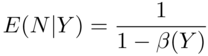
respectively. Thus,

and by substitution we get

Rewriting this expression in terms of integrals, we obtain the unconditional variance of the run‐length distribution in Case KU

where the reader should recall that ![]() , as defined earlier. Note that, although the run‐length distribution is always discrete, the monitored variable, and therefore the corresponding parameter estimator(s), can be continuous (as in the present case) as well as discrete, as in the case of attributes charts (see Montgomery, 2009, Chapter 7). In the latter case, the estimator Y will be discrete and thus the unconditional run‐length distribution, its average, and the variance can be obtained in a similar manner using the CUC method, except that now the integral will be replaced by summation over the mass points of the estimator Y, and the chi‐square pdf in the integration will be replaced by the appropriate pmf of Y. The reader is referred to Human and Chakraborti (2006) for examples.
, as defined earlier. Note that, although the run‐length distribution is always discrete, the monitored variable, and therefore the corresponding parameter estimator(s), can be continuous (as in the present case) as well as discrete, as in the case of attributes charts (see Montgomery, 2009, Chapter 7). In the latter case, the estimator Y will be discrete and thus the unconditional run‐length distribution, its average, and the variance can be obtained in a similar manner using the CUC method, except that now the integral will be replaced by summation over the mass points of the estimator Y, and the chi‐square pdf in the integration will be replaced by the appropriate pmf of Y. The reader is referred to Human and Chakraborti (2006) for examples.
Other moments and characteristics of the run‐length distribution can also be obtained similarly using the CUC method, which takes advantage of the facts that (i) the conditional run‐length given the parameter estimate is the geometric distribution and (ii) the unconditioning involves averaging (taking expectation) over the distribution of the parameter estimator, which follows some known probability distribution.
Typically, one refers to the unconditional run‐length distribution as the run‐length distribution of a control chart, but the conditional run‐length distribution is gaining more prominence as it captures and explains the impact of the inherent variation in the parameter estimators on the performance of the control chart. The reader is referred to the recent literature for more details.
In summary, while the unconditional run‐length properties, such as the mean and the standard deviation, are fixed, and describe the average performance of the control chart over many reference samples, the conditional run‐length properties vary based on the values of the parameter estimators for a given reference sample and show the impact of parameter estimation based on the value of the estimator that the users have for their particular situation. Both the conditional and the unconditional performance may have a role to play in the practical implementation of control charts with estimated parameters. The Case KK run‐length distribution and its associated characteristics have been the benchmarking norm in the design of a control chart for over 50 years, until recently, when the unconditional run‐length and its associated characteristics gained prominence in light of the effects of parameter estimation, but, as noted earlier, it is recognized that, although the averaging process may produce some useful overall guidance, the conditional run‐length and its associated characteristics may be very useful while implementing and understanding chart performance in practice when estimated parameters are used in control charts. The same summary applies to all types of control charts, univariate or multivariate, variables or attributes, parametric or nonparametric, where unknown parameters are estimated from the data.
Next, consider the case when both parameters are unknown, that is, Case UU. The analysis is similar to that in Case KU, except that now two parameters and their corresponding estimators are involved, which raises the complexity. We will try to point out the similarities with Case KU and highlight the main differences. As we noted earlier, in Phase II, the parameter estimators and hence the control limits are obtained from Phase I and are applied to monitor the status of the process in Phase II on an ongoing basis. Again, as in Case KU, assume that in Phase I the process follows a normal distribution so that ![]() for
for ![]() and
and ![]() . In addition, we assume that we estimate the unknown IC process mean
. In addition, we assume that we estimate the unknown IC process mean ![]() and the unknown IC process standard deviation
and the unknown IC process standard deviation ![]() with the overall mean which is the grand mean of the means of the reference samples
with the overall mean which is the grand mean of the means of the reference samples

and the pooled estimator

Thus, unlike in Case KU, two estimators, namely ![]() and
and ![]() , are involved in the analysis in Case UU. Note also that, unlike in Case KU, the estimator of
, are involved in the analysis in Case UU. Note also that, unlike in Case KU, the estimator of ![]() , namely
, namely ![]() , has a scaled chi‐square distribution but with
, has a scaled chi‐square distribution but with ![]() , degrees of freedom. Thus, one loses
, degrees of freedom. Thus, one loses ![]() degrees of freedom (recall that in Case KU the degree of freedom was
degrees of freedom (recall that in Case KU the degree of freedom was ![]() ) while estimating the mean
) while estimating the mean ![]() using the
using the ![]() Phase I samples.
Phase I samples.
Again, the two‐sided control limits are given by substituting the point estimators in the control limits for Case KK

As before, assume that the Phase II samples follow an ![]() distribution. Thus, the signaling events in Phase II can be written as
distribution. Thus, the signaling events in Phase II can be written as
which can be re‐expressed as

Compare this signaling event with that in Case KU. As in Case KU, under the CUC method, the probability of a signaling event in Case UU is calculated in two steps. First, the probability of a signal is calculated given (conditioned on) the two parameter estimators, ![]() and
and ![]() , which are both random variables. This probability is called the conditional probability of a signal and it plays a key role in the subsequent developments.
, which are both random variables. This probability is called the conditional probability of a signal and it plays a key role in the subsequent developments.
To show this, we note that the probability of a signal in Case UU is given by  for
for ![]() This can be written as
This can be written as

Now, writing ![]() ,
, ![]() , and
, and ![]() , we can rewrite the above probability as
, we can rewrite the above probability as
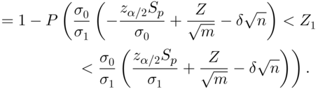
Finally, writing ![]() , which follows a chi‐square distribution with
, which follows a chi‐square distribution with ![]() degrees of freedom and denoting
degrees of freedom and denoting ![]() , we can further rewrite the last expression as
, we can further rewrite the last expression as

When ![]() the quantity
the quantity ![]() . Finally, since
. Finally, since ![]() follows a N(0,1) distribution, the conditional probability of a signal in Phase II for the mean chart in Case UU is given by
follows a N(0,1) distribution, the conditional probability of a signal in Phase II for the mean chart in Case UU is given by

where ![]() and
and ![]() are independent random variables. The variable
are independent random variables. The variable ![]() follows a standard normal distribution and
follows a standard normal distribution and ![]() follows a chi‐square distribution with
follows a chi‐square distribution with ![]() degrees of freedom. Again, other estimators of
degrees of freedom. Again, other estimators of ![]() could be considered, and one would have to work with its distribution in the sequel. We leave this up to the reader.
could be considered, and one would have to work with its distribution in the sequel. We leave this up to the reader.
In any case, also in Case UU, the conditional probability of a signal plays an important role in the analysis of the performance of the control chart under estimated parameters. We comment more on this later. In the IC case, we have ![]() and under the typical assumption that
and under the typical assumption that ![]() , that is,
, that is, ![]() , the quantity
, the quantity ![]() denotes the IC conditional probability of a signal (the FAR) in Phase II. However, since this probability is a function of random variables
denotes the IC conditional probability of a signal (the FAR) in Phase II. However, since this probability is a function of random variables ![]() and
and ![]() , it is a random variable with its own probability distribution. This is why, as we noted earlier, when parameters are estimated in Phase II, typically, one does not use the FAR to describe chart performance since the FAR depends on the type of estimates obtained from the Phase I analysis and is itself a random variable with a probability distribution.
, it is a random variable with its own probability distribution. This is why, as we noted earlier, when parameters are estimated in Phase II, typically, one does not use the FAR to describe chart performance since the FAR depends on the type of estimates obtained from the Phase I analysis and is itself a random variable with a probability distribution.
Moreover, as in Case KU, the Phase II signaling events are dependent in Case UU due to the fact that the same Phase I parameter estimates in the control limits and each Phase II sample is compared with the same control limits involving these estimates. Thus, in Case UU, as in Case KU, the run‐length distribution of the Phase II control chart no longer follows a geometric distribution since the Bernoulli trials involved in this case are no longer independent. However, again, as in Case KU, given the Phase I parameter estimators (or conditioning over the corresponding random variables), the signaling events are independent. This observation facilitates a lot of the statistical calculations of the Phase II chart properties in Case UU, as it did in Case KU. Thus, to summarize, in Case UU, for the Shewhart ![]() chart,
chart,
- The conditional Phase II run‐length distribution is geometric with success probability
 .
. - Hence, conditionally, properties of the Phase II Shewhart
 chart follow from the properties of the geometric distribution, for example, the conditional run‐length distribution is given by its probability mass function (pmf)
where we write, for brevity,
chart follow from the properties of the geometric distribution, for example, the conditional run‐length distribution is given by its probability mass function (pmf)
where we write, for brevity,
 . Now, using properties of the geometric distribution, we can easily obtain various attributes of the conditional run‐length distribution. The conditional average run‐length (
 ) of the Phase II chart, for example, is given by
  . Similarly, the variance and the standard deviation are given by
  and
and  , respectively.
As noted earlier, parameter estimates plugged into the control limits can significantly alter/affect the performance of the control chart and the conditional run‐length distribution. Its associated characteristics, such as the average, the standard deviation, etc., can help to describe the effects of parameter estimation on the performance of the Phase II control chart. The estimators are random variables, and two independent reference samples from the same IC process would most likely produce two different sets of parameter estimates, which in turn will produce different control charts (limits), and hence different Phase II chart performance. The bottom line is that there will be variation in the performance of the control charts among users, when they use estimates from independent reference samples from the same IC process, and even though the control charts may have been calibrated to achieve the same nominal ARLIC. This variation may be termed as user‐to‐user variation, which is not easy to control unless there are lots of data, which may not be practical in all situations. To this end, as noted before, several recent articles have suggested studying the conditional run‐length distribution and the impact of user‐to‐user variation on Phase II control charts. We cover some of these aspects in later chapters.
Averaging over the distributions of the parameter estimates, a process known as “unconditioning,” we can study the “average” chart performance, for example, the unconditional probability of a signal in Case UU is given by

where ![]() denotes the pdf of a chi‐square distribution with
denotes the pdf of a chi‐square distribution with ![]() degrees of freedom. Note that for the normal distribution the estimators of the mean and the variance are statistically independent. Therefore, the joint distribution factors into the product of the individual distributions, one a standard normal and one a chi‐square. This may not be the situation in all cases, however. Similarly, using the CUC method, the unconditional run‐length pmf can be obtained by integrating the conditional run‐length pmf over the joint pdf of
degrees of freedom. Note that for the normal distribution the estimators of the mean and the variance are statistically independent. Therefore, the joint distribution factors into the product of the individual distributions, one a standard normal and one a chi‐square. This may not be the situation in all cases, however. Similarly, using the CUC method, the unconditional run‐length pmf can be obtained by integrating the conditional run‐length pmf over the joint pdf of ![]() and
and ![]() , which is the product of the marginal pdf's of
, which is the product of the marginal pdf's of ![]() and
and ![]() , respectively since
, respectively since ![]() and
and ![]() are independent. Hence
are independent. Hence

Similarly, using the fact that the conditional run‐length distribution is geometric with a success probability ![]() , and applying the CUC method, the expected value of the unconditional run‐length distribution is given by
, and applying the CUC method, the expected value of the unconditional run‐length distribution is given by

This is the unconditional ARL of the Shewhart ![]() control chart in Case UU. In general, for higher‐order moments, say, the
control chart in Case UU. In general, for higher‐order moments, say, the ![]() non‐central moment of the run‐length distribution can be obtained from the
non‐central moment of the run‐length distribution can be obtained from the ![]() conditional non‐central moment, that is,
conditional non‐central moment, that is, ![]() using the fact that
using the fact that ![]() follows a geometric distribution. In particular, the variance (or the standard deviation) of the unconditional run‐length distribution is an important performance measure. This can be shown to be equal to
follows a geometric distribution. In particular, the variance (or the standard deviation) of the unconditional run‐length distribution is an important performance measure. This can be shown to be equal to ![]()
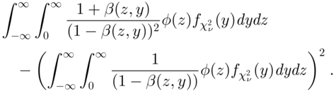
The derivation of the unconditional variance (and standard deviation) is interesting and is explained further. This follows from the result that for any random variable N, ![]() (see, for example, Hogg, McKean, and Craig, 2005) where the expectation is taken over the distributions of the two independent random variables
(see, for example, Hogg, McKean, and Craig, 2005) where the expectation is taken over the distributions of the two independent random variables ![]() and
and ![]() . Furthermore, under the assumption of a normal distribution,
. Furthermore, under the assumption of a normal distribution, ![]() and
and ![]() are independent. For the
are independent. For the ![]() and the
and the ![]() terms, we note that, given
terms, we note that, given ![]() and
and ![]() , the run‐length distribution is geometric with probability
, the run‐length distribution is geometric with probability ![]() and hence from the properties of the geometric distribution,
and hence from the properties of the geometric distribution, ![]() and
and ![]() . Thus
. Thus

and by substitution we get

Rewriting this expression in terms of integrals, we obtain the unconditional variance

shown above. Hence, the unconditional run‐length standard deviation is given by ![]() .
.
Typically, one refers to the unconditional run‐length distribution as the run‐length distribution of a control chart, which has been used in the traditional evaluation of a control chart performance. However, the conditional run‐length distribution has gained more prominence recently as it captures and explains the impact of the inherent variation in the parameter estimators on the performance of the control chart. Other moments and characteristics of the run‐length distribution can be obtained similarly using the CUC method, which takes advantage of the facts that (i) the conditional run‐length given the parameter estimates is the geometric distribution, and (ii) the unconditioning involves averaging (taking expectation) over the distributions of the two parameter estimators, which are independent, and follows some known probability distributions. In summary, while the unconditional run‐length properties, such as the mean and the standard deviation, are fixed and describe the average performance of the control chart over many samples, the conditional run‐length properties are not and show the impact of parameter estimation based on the estimators that the users have for their situation. Both conditional and unconditional performance may have a role to play in the practical implementation of control charts with estimated parameters.
For Case UK, the probability of a signal, the conditional run‐length distribution, its various moments, the unconditional run‐length distribution, and its various moments can be obtained similarly and are left for the reader as exercises. More details can be found in Chakraborti (2000).
Having considered the Shewhart chart for the mean in detail, we are now in a better position to study some of the more advanced or sophisticated charts. These include the CUSUM and the EWMA charts, and Shewhart charts with supplementary runs‐rules, which are expected to be more effective in detecting small, persistent changes in the underlying parameter. The calculation of the run‐length distribution and associated properties for these charts are more involved in Case U, but one can again apply the CUC method. This is briefly outlined as follows, first in general terms. Recall that, for these charts, expressions for the run‐length distribution and some of the associated characteristics in Case K were given in Equations 3.21
,3.22,3.23,3.24 using the MC approach. This is the starting point in Case U. As we noted earlier, a key to using these expressions is the construction of the essential transition probability matrix for each chart. In Case U, we first use these formulas conditionally given the parameter estimates, and then apply the CUC method to find the unconditional run‐length distribution and its associated properties. Suppose, for example, that there is a single unknown parameter to be estimated with the corresponding Phase I estimator ![]() . Now we calculate the elements of the essential probability matrix
. Now we calculate the elements of the essential probability matrix ![]() , the so‐called transition probabilities, by using the conditional distribution of the charting statistic in Phase II, given the estimator
, the so‐called transition probabilities, by using the conditional distribution of the charting statistic in Phase II, given the estimator ![]() . Thus, each element of the transition probability matrix is calculated conditional on
. Thus, each element of the transition probability matrix is calculated conditional on ![]() , and let
, and let ![]() denote the resulting conditional essential probability matrix. Next, we can apply the expressions given in Equations 3.22
,3.23,3.24 conditionally on
denote the resulting conditional essential probability matrix. Next, we can apply the expressions given in Equations 3.22
,3.23,3.24 conditionally on ![]() , and get
, and get
Finally, using the CUC method, the unconditional run‐length distribution is obtained by taking the expectation (averaging or integrating) over the distribution of ![]() . So, for example, the unconditional
. So, for example, the unconditional ![]() of the chart is given by
of the chart is given by

where ![]() is assumed to be continuous with a pdf
is assumed to be continuous with a pdf ![]() . Other moments and associated run‐length distribution characteristics can be found in a similar manner. Note that a similar analysis is possible if case
. Other moments and associated run‐length distribution characteristics can be found in a similar manner. Note that a similar analysis is possible if case ![]() is discrete, in which case one would obtain these expressions for the unconditional run‐length distribution by summing over the pmf
is discrete, in which case one would obtain these expressions for the unconditional run‐length distribution by summing over the pmf ![]() of
of ![]() . Interested readers are asked to try out some examples. Some examples can be found in Chakraborti, Eryilmaz and Human (2009).
. Interested readers are asked to try out some examples. Some examples can be found in Chakraborti, Eryilmaz and Human (2009).
3.10.1.2 The Shewhart Chart for the Variance in Case U
The run‐length distribution of the Shewhart charts for the variance can be obtained similarly, as in the case of the mean, using the CUC method. We sketch a brief example here for the ![]() chart with
chart with ![]() as the estimator of
as the estimator of ![]() and derive the IC run‐length distribution.
and derive the IC run‐length distribution.
Note that, in this case, the probability limits of the Phase II chart are given by ![]() ,
, ![]() , and
, and ![]() , where
, where ![]() ,
, ![]() , and
, and ![]() is the unconditional probability that the Phase II charting statistic, the standard deviation,
is the unconditional probability that the Phase II charting statistic, the standard deviation, ![]() plots outside either the lower or the upper control limit when the process is IC. Note that, in the parameter known case, this is the probability of a false alarm or the FAR and it only depends on the sample size n, but in the unknown parameter case, the probability
plots outside either the lower or the upper control limit when the process is IC. Note that, in the parameter known case, this is the probability of a false alarm or the FAR and it only depends on the sample size n, but in the unknown parameter case, the probability ![]() depends on both m and n. Once the quantity
depends on both m and n. Once the quantity ![]() is determined, the probability limits are easily obtained using the corresponding percentiles of the chi‐square distribution with
is determined, the probability limits are easily obtained using the corresponding percentiles of the chi‐square distribution with ![]() degrees of freedom. Although we may refer to
degrees of freedom. Although we may refer to ![]() as the FAR (probability of a signal when the process is IC) in Case U, for convenience, note that it does not have the same clear interpretation as in Case K since the signaling events are dependent in Case U. Some details about the derivation of
as the FAR (probability of a signal when the process is IC) in Case U, for convenience, note that it does not have the same clear interpretation as in Case K since the signaling events are dependent in Case U. Some details about the derivation of ![]() are given in Appendix 3.3. The
are given in Appendix 3.3. The ![]() values are calculated and shown in Table H in Appendix A along with the corresponding control limits
values are calculated and shown in Table H in Appendix A along with the corresponding control limits ![]() and
and ![]() for n = 5 and 10 and some values of m from 5 to 100, with nominal ARLIC values of 370 and 500. Note that the
for n = 5 and 10 and some values of m from 5 to 100, with nominal ARLIC values of 370 and 500. Note that the ![]() values depend both on m and n, and for a given value of n, they increase for increasing values of m (increasing the number of Phase I samples).
values depend both on m and n, and for a given value of n, they increase for increasing values of m (increasing the number of Phase I samples).
Other moments of the conditional and the unconditional IC run‐length distribution can be found in a similar way. Note that when other estimators of ![]() , such as the one based on the
, such as the one based on the ![]() or the
or the ![]() are used in the Phase I control limits, or a different chart such as the R chart is used in Phase II, a similar approach can be used to derive the run‐length distribution and its various moments by applying the CUC method. We basically need the probability distributions of the charting statistic and of the Phase I estimator of
are used in the Phase I control limits, or a different chart such as the R chart is used in Phase II, a similar approach can be used to derive the run‐length distribution and its various moments by applying the CUC method. We basically need the probability distributions of the charting statistic and of the Phase I estimator of ![]() . Note that the same approach can be also used to derive the OOC run‐length distribution, which is useful in studying the performance of these charts in shift detection and comparisons. We leave the details to the reader.
. Note that the same approach can be also used to derive the OOC run‐length distribution, which is useful in studying the performance of these charts in shift detection and comparisons. We leave the details to the reader.
3.10.1.3 The CUSUM Chart for the Mean in Case U
The reader is referred back to Example 3.6 in Section 3.6.1.2. In this example, the underlying process distribution is assumed to be N(0,1). Let us consider, for example, the one‐step transition probability, ![]() . It was shown that
. It was shown that ![]() . However, recall that the
. However, recall that the ![]() was obtained using the cdf of a N(0,1) distribution, which requires not only the knowledge of the normality of the process distribution but also that the mean and the standard deviation, assumed to be 0 and 1, respectively. Suppose now that we are in Case KU, that is, the process mean is known (say, is equal to zero), but the process variance is unknown. In this case, we have a single unknown parameter
was obtained using the cdf of a N(0,1) distribution, which requires not only the knowledge of the normality of the process distribution but also that the mean and the standard deviation, assumed to be 0 and 1, respectively. Suppose now that we are in Case KU, that is, the process mean is known (say, is equal to zero), but the process variance is unknown. In this case, we have a single unknown parameter ![]() to be estimated by some estimator
to be estimated by some estimator ![]() (which is typically obtained from a Phase I analysis) and we calculate the elements of the essential probability matrix
(which is typically obtained from a Phase I analysis) and we calculate the elements of the essential probability matrix ![]() , that is, the transition probabilities, conditionally, given the estimator
, that is, the transition probabilities, conditionally, given the estimator ![]() . Now
. Now ![]() is calculated as
is calculated as ![]() where
where ![]() is some estimator of
is some estimator of ![]() . The same applies to the other one‐step transition probabilities. Thus,
. The same applies to the other one‐step transition probabilities. Thus, ![]() , the estimated conditional essential probability matrix, is obtained and substituted into Equations 3.36,3.37,3.38,3.39. Finally, using the CUC method, the unconditional run‐length distribution is obtained by taking expectation over the distribution of
, the estimated conditional essential probability matrix, is obtained and substituted into Equations 3.36,3.37,3.38,3.39. Finally, using the CUC method, the unconditional run‐length distribution is obtained by taking expectation over the distribution of ![]() , as explained above and illustrated in Equation 3.40 for the unconditional ARL. Case UK follows similarly. However, this time the process mean needs to be estimated and dealt with and, for Case UU, where both the process mean and the process variance need to be estimated, we condition on, say,
, as explained above and illustrated in Equation 3.40 for the unconditional ARL. Case UK follows similarly. However, this time the process mean needs to be estimated and dealt with and, for Case UU, where both the process mean and the process variance need to be estimated, we condition on, say, ![]() and
and ![]() , where
, where ![]() denotes the estimator for the process mean and
denotes the estimator for the process mean and ![]() denotes the estimator for the process variance. The reader is also referred to Jones, Champ, and Rigdon (2004) for an alternative derivation of the run‐length distribution of the CUSUM chart with estimated parameters.
denotes the estimator for the process variance. The reader is also referred to Jones, Champ, and Rigdon (2004) for an alternative derivation of the run‐length distribution of the CUSUM chart with estimated parameters.
3.10.1.4 The EWMA Chart for the Mean in Case U
The reader is referred back to Example 3.7 in Section 3.6.1.2
. In this example, the underlying process distribution is assumed to be N(0,1). Let us consider the one‐step transition probability, ![]() , in that example. It was shown that
, in that example. It was shown that ![]() is equal to
is equal to ![]() but
but ![]() is obtained using the cdf of a N(0,1) distribution. However, even when we assume normality, one or more of the parameters can be unknown and would need to be estimated. In such a case, we proceed as in the case of the CUSUM chart discussed above, and calculate the elements of the transition probability matrix conditioned on the parameter estimators. Then, the resulting conditional essential probability matrix is obtained and substituted into Equations 3.36
,3.37,3.38,3.39. Finally, using the CUC method, the unconditional run‐length distribution is obtained by taking expectation over the distribution of the estimator(s), as explained above and illustrated in Equation 3.40
for the unconditional ARL. The reader is referred to Jones, Champ, and Rigdon (2001) for a detailed discussion on the run‐length distribution of the EWMA chart with estimated parameters.
is obtained using the cdf of a N(0,1) distribution. However, even when we assume normality, one or more of the parameters can be unknown and would need to be estimated. In such a case, we proceed as in the case of the CUSUM chart discussed above, and calculate the elements of the transition probability matrix conditioned on the parameter estimators. Then, the resulting conditional essential probability matrix is obtained and substituted into Equations 3.36
,3.37,3.38,3.39. Finally, using the CUC method, the unconditional run‐length distribution is obtained by taking expectation over the distribution of the estimator(s), as explained above and illustrated in Equation 3.40
for the unconditional ARL. The reader is referred to Jones, Champ, and Rigdon (2001) for a detailed discussion on the run‐length distribution of the EWMA chart with estimated parameters.
In the unknown parameter case, the CUC method has been successfully used not only for various parametric charts but also for nonparametric charts, as will be seen in the next chapter.
3.11 Control Chart Enhancements
3.11.1 Run‐length Calculation for Runs‐type Signaling Rules in Case U
Zhang and Castagliola (2010) considered the Shewhart ![]() chart with runs rules when the process parameters are unknown. Recall that, if the IC process mean and standard deviation
chart with runs rules when the process parameters are unknown. Recall that, if the IC process mean and standard deviation ![]() and
and ![]() are both unknown, in Case UU, they are estimated from a Phase I reference data set of size m (
are both unknown, in Case UU, they are estimated from a Phase I reference data set of size m (![]() 1) subgroups, each of size n (
1) subgroups, each of size n (![]() 1). We can use the commonly used estimators
1). We can use the commonly used estimators ![]() and
and ![]() where recall that
where recall that ![]() is the mean of the Phase I sample means and
is the mean of the Phase I sample means and ![]() is the so‐called pooled estimator of the standard deviation. Let
is the so‐called pooled estimator of the standard deviation. Let ![]() denote a Phase II sample and let
denote a Phase II sample and let ![]() denote the mean of that sample. We now plug in the estimators into the well‐known Shewhart k‐sigma control limits and get the estimated limits
denote the mean of that sample. We now plug in the estimators into the well‐known Shewhart k‐sigma control limits and get the estimated limits ![]() as shown earlier. Since
as shown earlier. Since ![]() and
and ![]() are random variables,
are random variables, ![]() and
and ![]() are also random variables. The conditional signaling probabilities can be found as, namely,
are also random variables. The conditional signaling probabilities can be found as, namely, ![]() and
and ![]() so that
so that ![]() . By substituting
. By substituting ![]() into the expressions for
into the expressions for ![]() and
and ![]() we find
we find ![]() and
and ![]() , respectively. We don't discuss
, respectively. We don't discuss ![]() in detail from this point forward because it can be found using
in detail from this point forward because it can be found using ![]() . By subtracting the Phase II mean
. By subtracting the Phase II mean ![]() and dividing each side of the inequalities by
and dividing each side of the inequalities by ![]() we find
we find

and

respectively.
By definition, under the assumption that the Phase II distribution has a mean shift, ![]() , so that we can write the above expressions in terms of the cdf of the standard normal distribution
, so that we can write the above expressions in terms of the cdf of the standard normal distribution

and

respectively.
Define the random variables ![]() and
and ![]() , respectively. Now we can write the signaling probabilities in a simpler format, namely
, respectively. Now we can write the signaling probabilities in a simpler format, namely
respectively. The pdf of the random variable ![]() is equal to
is equal to ![]() , where
, where ![]() is the pdf of the standard normal distribution, since
is the pdf of the standard normal distribution, since
For the random variable ![]() , we make use of the fact that
, we make use of the fact that
so that
and hence the pdf of ![]() is given by
is given by
where ![]() is the pdf of a gamma distribution with parameters
is the pdf of a gamma distribution with parameters ![]() and
and ![]() , respectively. This line of derivation is based on Zhang and Castagliola (2010) but one can also follow Chakraborti (2000) and rewrite the equations in terms of the more familiar chi‐square distribution.
, respectively. This line of derivation is based on Zhang and Castagliola (2010) but one can also follow Chakraborti (2000) and rewrite the equations in terms of the more familiar chi‐square distribution.
The unconditional properties of the run‐length distribution can now be found using the CUC technique discussed in Section 3.7. The idea we wanted to introduce here is that the CUC technique discussed in Section 3.10.1 can also be conveniently used for charts with runs‐type signaling rules. Note that as alluded to earlier, since the random variable ![]() can be rescaled so that its distribution may be written in terms of a chi‐square distribution, the above expressions can be rewritten in terms of the chi‐square distribution with some appropriate degrees of freedom. This may be more useful from a practical point of view since the chi‐square pdf is more readily available. We leave the verification of these details to the reader.
can be rescaled so that its distribution may be written in terms of a chi‐square distribution, the above expressions can be rewritten in terms of the chi‐square distribution with some appropriate degrees of freedom. This may be more useful from a practical point of view since the chi‐square pdf is more readily available. We leave the verification of these details to the reader.
3.12 Phase I Control Charts
3.12.1 Phase I  ‐chart
As discussed earlier, Phase I analysis is a very important part of the overall SPC regime, and control charts, particularly Shewhart charts, play an important role in monitoring the Phase I subgroup. In this section we first discuss the Phase I ![]() ‐chart. Suppose there are m Phase I subgroups each of size n, and
‐chart. Suppose there are m Phase I subgroups each of size n, and ![]() denotes the jth observation from the ith subgroup. Let
denotes the jth observation from the ith subgroup. Let ![]() and
and ![]() denote the mean and the variance, respectively, of the ith subgroup. The charting statistic for the Phase I
denote the mean and the variance, respectively, of the ith subgroup. The charting statistic for the Phase I ![]() ‐chart is the mean,
‐chart is the mean, ![]() , of each subgroup and the control limits are given by
, of each subgroup and the control limits are given by
where ![]() is the overall (or the grand) mean and
is the overall (or the grand) mean and ![]() is an unbiased estimator of the process standard deviation, based on the average subgroup variances with the constant
is an unbiased estimator of the process standard deviation, based on the average subgroup variances with the constant ![]() (see Table C in Appendix A). The constant
(see Table C in Appendix A). The constant ![]() is the chart design constant which is determined for a given nominal FAP value, m and n. Champ and Jones (2004) discussed this problem for a number of standard deviation estimators including the
is the chart design constant which is determined for a given nominal FAP value, m and n. Champ and Jones (2004) discussed this problem for a number of standard deviation estimators including the ![]() above and show that
above and show that ![]() can be obtained from the cdf of a multivariate t distribution with a special correlation structure. The interested reader is referred to their paper for more details. They tabulated the constant
can be obtained from the cdf of a multivariate t distribution with a special correlation structure. The interested reader is referred to their paper for more details. They tabulated the constant ![]() for
for ![]() , and
, and ![]() and a nominal FAP of 0.01, 0.05, and 0.10. However, recently, the number of Phase I subgroups,
and a nominal FAP of 0.01, 0.05, and 0.10. However, recently, the number of Phase I subgroups, ![]() , is recommended to be much larger, say, 50 or even 100 or more in order to properly account for parameter estimation. Champ and Jones (2004) also discussed some approximations for
, is recommended to be much larger, say, 50 or even 100 or more in order to properly account for parameter estimation. Champ and Jones (2004) also discussed some approximations for ![]() when
when ![]() is large; however, recent advances in computer software available for the calculation of the cdf of the multivariate normal and the multivariate t distribution now make it possible to calculate
is large; however, recent advances in computer software available for the calculation of the cdf of the multivariate normal and the multivariate t distribution now make it possible to calculate ![]() exactly for large values of
exactly for large values of ![]() , even for
, even for ![]() . Recently, Yao et al. (2017) has extended their tables to larger values of
. Recently, Yao et al. (2017) has extended their tables to larger values of ![]() and has provided an
and has provided an ![]() package to make the calculations on demand.
package to make the calculations on demand.
3.13 Size of Phase I Data
The Phase I reference data set is typically made up of m (![]() 1) subgroups, each of size n (
1) subgroups, each of size n (![]() 1). Thus, there is a total of mn Phase I observations (reference data) available for parameter estimation and for setting up the control limits which are used in Phase II. There are generally two approaches to obtaining a Phase I reference data set. It may be that it is already available (as a retrospective or a historical data set) or that the process needs to be first brought IC and then reference data are gathered. Getting a process IC and thus obtaining the reference data involves a careful Phase I analysis (where the control limits are viewed as trial limits and are used iteratively, until the charting statistics all plot IC) including the use of control charts and other statistical tools. The readers are referred to Jones‐Farmer et al. (2014) and Chakraborti, Human, and Graham (2009) for more details about Phase I control charting. The bottom line is that the effects of parameter estimation are real, it varies from practitioner to practitioner and often result in more false alarms than what is nominally expected. If a large number of reference data are available, the Phase II limits can perform like their known parameter counterparts. Conversely, the control limits can be calculated for the data at hand. The underlying issues include knowledge of the form/shape of the underlying distribution, the parameter of interest, the type of estimator, the type of chart, and so on. When estimating process variability, for example, one typically needs much larger sample sizes than when estimating the process mean. Recall that (from the Phase I and Phase II analyses discussion in Section 2.1.12) one of the major goals of a Phase I analysis is to estimate process variability.
1). Thus, there is a total of mn Phase I observations (reference data) available for parameter estimation and for setting up the control limits which are used in Phase II. There are generally two approaches to obtaining a Phase I reference data set. It may be that it is already available (as a retrospective or a historical data set) or that the process needs to be first brought IC and then reference data are gathered. Getting a process IC and thus obtaining the reference data involves a careful Phase I analysis (where the control limits are viewed as trial limits and are used iteratively, until the charting statistics all plot IC) including the use of control charts and other statistical tools. The readers are referred to Jones‐Farmer et al. (2014) and Chakraborti, Human, and Graham (2009) for more details about Phase I control charting. The bottom line is that the effects of parameter estimation are real, it varies from practitioner to practitioner and often result in more false alarms than what is nominally expected. If a large number of reference data are available, the Phase II limits can perform like their known parameter counterparts. Conversely, the control limits can be calculated for the data at hand. The underlying issues include knowledge of the form/shape of the underlying distribution, the parameter of interest, the type of estimator, the type of chart, and so on. When estimating process variability, for example, one typically needs much larger sample sizes than when estimating the process mean. Recall that (from the Phase I and Phase II analyses discussion in Section 2.1.12) one of the major goals of a Phase I analysis is to estimate process variability.
To summarize, an accurate and precise estimation of parameters in Phase I is critical for the satisfactory performance of the control chart in the monitoring phase, namely, Phase II, as the run‐length properties are greatly impacted by estimation, which can lead to, for example, many more false alarms than are nominally expected based on the pre‐set IC average run‐length; see, for example, Jensen et al. (2006) and Psarakis, Vyniou, and Castagliola (2014). These and other authors have concluded that the number of the Phase I samples, ![]() , must often be quite large (in many hundreds of observations) in order to have reasonable confidence that the performance of the control chart will be close to that of the known performance in Case K or KK. Note that there is no magic number for
, must often be quite large (in many hundreds of observations) in order to have reasonable confidence that the performance of the control chart will be close to that of the known performance in Case K or KK. Note that there is no magic number for ![]() since the choice of
since the choice of ![]() depends largely on the type of control chart to be implemented and the parameter estimators employed. Some work in the literature (e.g., Chakraborti, 2006; Saleh et al., 2015; Epprecht, Loureiro, and Chakraborti, 2016) explores the various issues and shows that it takes a much larger Phase I sample size, often a few times larger than what has been typically recommended in textbooks, to obtain consistent chart properties that are close to the known parameter case. The known parameter case is held as a standard since those values don't vary. Thus, one has to be very careful about starting a Phase II charting procedure with a limited amount of historical data. The other approach may be to adjust the control limits for the given amount of data at hand. More research on this topic is in progress.
depends largely on the type of control chart to be implemented and the parameter estimators employed. Some work in the literature (e.g., Chakraborti, 2006; Saleh et al., 2015; Epprecht, Loureiro, and Chakraborti, 2016) explores the various issues and shows that it takes a much larger Phase I sample size, often a few times larger than what has been typically recommended in textbooks, to obtain consistent chart properties that are close to the known parameter case. The known parameter case is held as a standard since those values don't vary. Thus, one has to be very careful about starting a Phase II charting procedure with a limited amount of historical data. The other approach may be to adjust the control limits for the given amount of data at hand. More research on this topic is in progress.
3.14 Robustness of Parametric Control Charts
A robust statistical procedure is a procedure that performs well not only under ideal conditions (under which it is designed and mathematically derived), but also with some departure from the ideal. An important question about a statistical hypothesis test is its Type‐I error robustness since without that the power properties of the test are questionable. In the same spirit, the IC robustness of a control chart is an important property that needs to be assessed and addressed since without it the shift detection performance of the chart is basically meaningless. The issue is serious with parametric charts since they are typically constructed under an assumed distribution (model) and hence their properties become suspect when that assumption doesn't hold or can't be adequately justified in a given situation. Many parametric charts, including the Shewhart, the CUSUM, and the EWMA charts, have been shown to suffer from a lack of IC robustness, to various degrees, under non‐normality. A consequence of this is that the IC average run‐length is shortened, so much so, that many more false alarms are observed than are nominally expected. This can reduce the efficacy of any control chart and hurt the entire monitoring regime. Although some authors have suggested that some parametric control charts can be designed (tuned) to be robust against a number of distributions (see Borror, Montgomery, and Runger, 1999, about the traditional parametric EWMA control chart), this, however, can be problematic as some knowledge about the shape of the distribution and the expected shift that are necessary for tuning may not always be available. In fact, Human, Kritzinger, and Chakraborti (2011) showed that the traditional parametric EWMA control chart can lack IC robustness for some non‐normal distributions such as the symmetric bi‐modal and the contaminated normal distribution. Their observations call into question routine applications of the traditional parametric EWMA control chart in practice. The issue of IC robustness can be a major concern for practitioners and, in such cases, nonparametric control charts can be applied. They are IC robust by definition since their IC run‐length distribution remains unchanged for all continuous distributions or continuous and symmetric distributions. This is one major practical advantage of the nonparametric charts. We recommend that, if the distributional assumption is in doubt or cannot be justified for lack of available information or data, a nonparametric or distribution‐free control chart should be used. This should be done even if there is a possibility of some loss of efficiency when the true model is correctly specified, since the true model is usually unknown.
Appendix 3.1 Some Derivations for the EWMA Control Chart
Appendix 3.2 Markov Chains
h3
The movement of a MC between the transient state(s) is interpreted (associated) as (with) the charting statistic moving in a stochastic manner on the control chart, without causing the chart to signal. This indicates that the process is (remains) IC and the state(s) associated with the process being IC is(are) identified with the transient state(s). There is a positive probability that the charting statistic can plot OOC at any point in time with the result that the chart gives a signal. The latter is equivalent to saying that the stochastic process ![]() has moved to an absorbing state (then the process cannot move back to any of the transient states). This means that once there is a signal on the chart the cause of the signal is identified and fixed and the process monitoring starts all over again from an IC state.
has moved to an absorbing state (then the process cannot move back to any of the transient states). This means that once there is a signal on the chart the cause of the signal is identified and fixed and the process monitoring starts all over again from an IC state.
Appendix 3.3 Some Derivations for the Shewhart Dispersion Charts
The charting constants for the Shewhart charts for the variance can be obtained in two steps. First, setting the unconditional IC average run‐length equal to some nominal value we solve for the probability ![]() . Then, in the second step, charting constants (and hence the control limits) for the Phase II dispersion charts are obtained from the corresponding percentiles of the chi‐square distribution (exactly or approximately) with n − 1 degrees of freedom. These limits are the unconditional probability limits. We sketch some details here using the S chart with Sp as the Phase I estimator of
. Then, in the second step, charting constants (and hence the control limits) for the Phase II dispersion charts are obtained from the corresponding percentiles of the chi‐square distribution (exactly or approximately) with n − 1 degrees of freedom. These limits are the unconditional probability limits. We sketch some details here using the S chart with Sp as the Phase I estimator of ![]() , using the CUC method. Note that in the section on the run‐length distribution, we showed that the probability limits are given by
, using the CUC method. Note that in the section on the run‐length distribution, we showed that the probability limits are given by ![]() and
and ![]() , where
, where ![]() is the probability that the charting statistic Si plots outside either the lower or the upper control limit when the process is IC. Thus, in order to get the charting constants
is the probability that the charting statistic Si plots outside either the lower or the upper control limit when the process is IC. Thus, in order to get the charting constants ![]() and
and ![]() , the
, the ![]() values are needed.
values are needed.
To this end, first note that

which can be re‐written as

where ![]() and
and ![]() are independent random variables and each follows a chi‐square distribution with (n – 1) and m(n– 1) degrees of freedom, respectively, in the IC case.
are independent random variables and each follows a chi‐square distribution with (n – 1) and m(n– 1) degrees of freedom, respectively, in the IC case.
The last probability can be calculated by conditioning on Sp or, equivalently on U. This is called the conditional false alarm rate (CFAR), which is a function of U, m, and n. Hence, the CFAR can be written as

so that the conditional run‐length distribution is geometric with probability CFAR (U,m,n,p). Thus, by applying the CUC method, the unconditional IC run‐length distribution (pmf) is given by
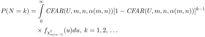
Note that this unconditional run‐length distribution is not geometric.
In a similar way, using the CUC method, the IC conditional average run‐length is given by ![]() and as such, the IC unconditional IC average run‐length is given by
and as such, the IC unconditional IC average run‐length is given by

Again, note that the ![]() is not the reciprocal of the CFAR. Now in the unconditional method setting the
is not the reciprocal of the CFAR. Now in the unconditional method setting the ![]() expression equal to some nominal value, such as 370, we solve the equation
expression equal to some nominal value, such as 370, we solve the equation ![]() numerically, for
numerically, for ![]() for given values of m and n. Then we find the 100*
for given values of m and n. Then we find the 100*![]() and the 100*[1 – α(m,n)/2] percentiles of a chi‐square distribution with n − 1 degrees of freedom. The required charting constants
and the 100*[1 – α(m,n)/2] percentiles of a chi‐square distribution with n − 1 degrees of freedom. The required charting constants ![]() and
and ![]() are found by dividing each of these percentiles by n − 1 and taking the square root. These values are shown in Table H in Appendix A. We leave the verification of the rest of this table for the other charts and with other Phase I estimators of σ to the reader.
are found by dividing each of these percentiles by n − 1 and taking the square root. These values are shown in Table H in Appendix A. We leave the verification of the rest of this table for the other charts and with other Phase I estimators of σ to the reader.
Finally, note that this formulation can accommodate a Phase II sample size, say, n1, not equal to the Phase I sample size m. The difference in this case will be in the degrees of freedom of the distribution of V, which will now be n1−1, in the first chi-square distribution, while defining the CFAR in Equation A3.6.