
Learning by neural networks
In this chapter, we describe algorithms for learning using neural networks. A neural network is a kind of computation system in which a state of the system is represented as a numerical distribution pattern with many processing units and connections among those units. Learning by neural networks uses an algorithm for transforming distribution patterns, which is quite different from learning based on symbolic representations described in Chapters 6–10. We will describe popular neural networks and explain methods for representing and using them for learning.
10.1 Representing neural networks
If we abstract a brain or the central nervous system of an animal, we can construct a model as a network where many neurons are densely connected with excitatory and inhibitory synapses. Furthermore, each of the neurons corresponding to the nodes of this network can be thought of as a function for transforming input information to another form of output. The efficiency of information transmission of the synapses that correspond to the edges of the network can be thought of as plastic, in the sense that the efficiency can change as the input information to the network changes. A state of the network can be represented as a numerical distribution pattern of the neurons’ states and the synapses’ information transmission efficiency over the network.
Furthermore, in this network, computation of the input-output function at each neuron and computation of the transmission efficiency change at each synaptic union can be done as a parallel process. Also, even if some of the neurons are broken, the state of the network as a whole and the output may not be influenced.
We can consider this structure, where the connectivity relation of many parallel processing units changes plastically, as one of the basic characteristics of the nervous system. Generally a dynamic network with these characteristics is called a neural network. neural networks can change the input-output relation by changing the state of a processing unit and the transmission efficiency of the unit. This is called learning in a neural network.
In this section, we will describe the representation of neural networks in preparation for explaining learning using neural networks. First, we define the general structure of the neural nets we are going to use in this chapter.
Definition 1
(neural network) Consider a set of processing units (called a unit from now on) U = {u1,…,un} and (directed) links between two units (called a link from now on) L = {(i, j)ui ∈ U, uj ∈ U} ⊆ U × U. Each unit receives input from other units joined by a link or from the outside and sends outputs to other units joined by a link or to the outside. The input-output relation at each unit ui can be defined as follows using the output function gi and the state transition function fi:
where aj(t) and Oj(t) represent the state of unit j at time t and the output from j at time t, respectively. Wji represents the weight of the link from unit i to j. We include the input function to unit j in the state transition function in the above definition. We represent the above definition as a five-tuple K = 〈U, L, W, O, F〉, where W is the set of the links’ weights, and O and F are the sets of the output and state transition functions. K is called a neural network.
The representation of units and links in a neural network is similar to the one for nodes and edges of a graph. Since each unit of a neural network is a function that depends on time, it can be regarded as an extended version of the graph representation described in Chapter 2.
[Example 1]
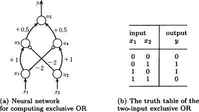
One example of neural networks is shown in Figure 10.1 (a). This example is a network made of five units and six links. The units u1 and u2 receive input only from the outside, u5 is a unit that sends output to the outside, and u3 and u4 are other units. The links (1,3) and (2,4) have weight 1, (3,5) and (4,5) have weight 0.5, and (1,4) and (2,3) have weight −2. Next, let us classify units.
Definition 2
(various units) A unit that receives input from the outside is called an input unit. A unit that sends output to the outside is called an output unit. A unit that is neither input nor output unit is called a hidden unit.
Definition 3
(various links) A link whose weight is nonnegative is called an excitatory link, and a link whose weight is negative is called an inhibitory link.
In Figure 10.1, the excitatory links are expressed using → and the inhibitory links are expressed using ⊷. For example, the link from unit u2 to u3 is inhibitory and has the weight w32 = −2.
[Example 2]
Consider a unit that has oi(t) = ai(t) as an output function and has the following state transition function:
This kind of unit is called a linear threshold unit. A neural network with layers of linear threshold units is known to possess computational power equivalent to that of a Turing machine. As an example, suppose the threshold value of each unit i in Figure 10.1(a) is θi = 0 (i = 1,…, 5). Then we can compute the exclusive OR using this neural network. For example when the input is x1(0) = 1, x2(0) = 1 we get a1(1) = 1, a2(1) = 1, a3(1) = 0, a4(1) = 0, a5(1) = 0, and the output y(1) = 0.
However, in the case of this version of exclusive OR, as the number of inputs increases, it becomes more and more difficult to find, within a practically reasonable time, the states and weights starting from arbitrarily given initial states and weights. The reason for this is that in the input-output relation of the exclusive OR, the input vector cannot be linearly separated according to the output values as intuitively shown in Figure 10.2.

[Example 3]
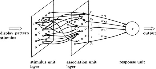
A simple three-layer perceptron is a network where a stimulus unit layer, an association unit layer, and one response unit are linked in series. Here we assume that the links from the stimulus unit layer to the association unit layer have random-valued weights and that all the association unit are linked to the response unit. Figure 10.3 shows an example. Let aji be the weight of the link from stimulus unit i to association unit j, wrj be the weight of the link from association unit j to the response unit r, and yj be the output from j to r. Furthermore, assume that the association units and the response unit are linear threshold units and that the threshold value of unit k is θk. Also, the output yj of association unit j is assumed as follows when the output from stimulus unit i to j is xji;

Also, we assume the following when the output of the response unit is or:

For the above neural network we want the response unit to output 1 when the input pattern is included in the set of patterns X and 0 when it is not included in X. This can be done by repeatedly changing the values of wrj (j = 1,…, n) by the fixed increment correction method given below.
Given a set of patterns X and a set of classes C, finding the subsets X1,…, Xk of X that correspond to c1,…,ck ∈ C respectively and satisfy ![]() is called pattern discrimination. When not all the classes c1,…, ck are known, this is called pattern classification. The example we look at here is an example of pattern discrimination where the set of classes is C = {0, 1}.
is called pattern discrimination. When not all the classes c1,…, ck are known, this is called pattern classification. The example we look at here is an example of pattern discrimination where the set of classes is C = {0, 1}.
Algorithm 10.1
(the fixed increment correction method)
[1] Suppose the set of patterns that can be input, P = {p1,…, pn}, is given. Also, for all the association units j, assign random values to wrj as the initial weights.
[2] Pick up an element of P, p, randomly and obtain the output from the response unit, oP, for the input pattern p.
[3] When the ideal output for p is rp, compute Δwrj = ∈(rp − op)xj for all the association units j, where ∈ is a positive constant that does not depend on the input pattern.
[4] Update the value of wrj using wrj = wrj + Δwrj for all the association units j.
[5] If the value of wrj no longer changes for all the input patterns p ∈ P, stop. The input patterns can be discriminated using wrj. Otherwise, go to [2].
Now, let ET be a subset of input patterns (whose ideal output from the response unit is 1), and let EF be the complementary set of ET for the set of all the possible input patterns (whose ideal output from the response unit is 0). Suppose ET and EF can be separated linearly. In other words, when an input pattern is represented by an n-dimensional vector, we assume that there is an (n − 1)-dimensional hyperplane aTy = b that makes aTy > b for all y ∈ ET, aTy ≤ b for all y ∈ EF. In this case, for a simple three-layer perceptron with the structure described above, if we take a small enough value of the step width ∈ when updating wrj in Algorithm 10.1, the algorithm converges in a finite number of iterations and we can find the weights wrj (j = 1, …, n) that make the discrimination of the input patterns possible. A rule for learning weights where the amount of change in the link weights is determined by the difference between the ideal output and the actual output is called a delta rule. The fixed increment correction method is a kind of delta rule.
10.2 Back Propagation
In the three-layer perceptron described in Section 10.1 [Example 3], it is difficult to learn to discriminate input patterns that cannot be separated linearly. More precisely, in such a three-layer perceptron, the number of units necessary for pattern discrimination depends on the size of the input pattern (for example, the dimension in a vector representation). However, there are many patterns that cannot be separated linearly, like the exclusive OR that was described in Example 2. We will explain the back propagation error learning algorithm as an algorithm for neural networks that learn to discriminate patterns that cannot be separated linearly.
(a) The structure of a neural network and an algorithm
Let us consider the neural network shown in Figure 10.4. This neural network has the following two features:

(1) It has a multilayer structure that has hidden-unit layers between the input-unit layer and the output-unit layer.
(2) It has a feedforward structure where links from the input-unit layer to the output-unit layer exist, but links in reverse directions do not exist.
Consider the following learning algorithm for neural networks with this structure. Suppose pairs of the input data and their ideal output are given in order. If we do the input-output computation for each unit using the neural network on these input data, we can obtain the actual output value. So, based on the error between the ideal output value and the actual output value for the same input datum, we change the weights of the links in the net so that the actual output value comes close to the ideal output value.
The problem here is whether, when we do this operation for each input, we can eventually learn the weights that output the ideal output value for arbitrary inputs.
The following algorithm gives a “weak” answer to this problem, “weak” meaning that the algorithm gives the steepest descent direction* that makes the sum of the squares of the error local minimum for the weights of the links. This does not guarantee that the algorithm converges in a finite number of steps or that it converges to the global minimum. However, from experience we know that, for networks up to reasonable sizes, we often can obtain weights that make the error between the actual output value and the ideal output value small using this algorithm. This algorithm can be thought of as a kind of algorithm for supervised learning in the sense that the ideal output value is given from outside.
Definition 4
(symbols for the algorithm) First, we define the output error of the output unit f for the kth input-output data (the pair of the input datum and its ideal output value) by
where we assume that rkj and okj are the ideal output value and the actual output value of the jth output unit for the kth input-output data, respectively, and that they take nonnegative values. ikj is the weighted sum of the outputs from each unit that are input to the jth unit in learning using the kth input-output data and can be defined as
where the ith unit is an input unit, and wki = xki (xki is the value of the ith element of the input pattern in the kth input-output data).
The function hj has the following meaning. When the output function of the unit j is simply
where akj is the state of unit j for the kth input-output data, and the state transition function is
we incorporate all of this and write
In other words, hj is the composite function of the output function gj and the state transition function fj, and matches fj exactly under the definition of (10.3) and (10.4). We assume that hj (in other words fj) is a nonlinear differentiable monotonically nondecreasing function and h’j is the derivative of hj. The condition of being nonlinear is necessary to make the propagation of the error become effective since the following algorithm is a method that is linear in the error.
Next, for a hidden unit, we define the output error of unit j for the kth input-output data as
(10.6) is a recursive expression where the output error of the hidden unit j is determined using the output error of other units that are directly linked to j. (10.1) and (10.6) together are called a generalized delta rule.
Using these definitions, the change in the link weight wji for the kth input-output data is given by
where α is a constant. Using (10.1), (10.6), and (10.7), the amount of change in the weights of all links can be computed using the following algorithm.
Algorithm 10.2
(back propagation error learning)
[1] Compute the output of each unit for the presented input in order from the input layer to the output layer (since the net does not include feedback links, this can be done easily).
[2] Compare the output okj of each output unit j against the presented ideal output value rkj and compute the output error δkj for each output unit j using (10.1).
[3] For each output unit j, compute the amount of change to the link weights that are directly connected to j from δkj and the actual output okj using (10.7).
[4] Change the weights of all the links that enter each output unit j, wji, to wji + Δkwji. Another method for obtaining the weight at time t + 1, wji(t + 1), is to add the weight at time t − 1, wji(t − 1), and set
The latter method smooths the changes of the weights and often avoids oscillation.
[5] Compute the output error δkj using (10.6) for each hidden unit j that is in the layer one layer closer to the input layer from the output layer.
[6] Compute the changes in the weights of the links that directly enter j, Δkwji, using (10.7) from δkj and the actual output oki for each hidden unit j computed in [5].
[7] Change the weights of all the links that enter j, wji, to wji + Δkwji for each hidden unit j computed in [6]. Similarly to [4], the weight at time t + 1 can also be obtained by adding the weight at time t − 1, wji(t − 1), and setting wji(t + 1) = wji(t) + Δkwji(t) − βwji(t − 1). In this way, we can smooth the changes of the weights.
[8] Do the same computation as in [5], [6], [7] for all the hidden units in order from the hidden layer closer to the output layer toward the input layer.
[9] Do [1]-[8] for each input-output data repeatedly changing the weights. The order of presenting the data can be fixed or can be random. When the square sum of the output error for the datum that is input last, Σj ![]() , is smaller than a given threshold value for each input-output data, stop. The learning is completed. Note that there are many other stopping criteria.
, is smaller than a given threshold value for each input-output data, stop. The learning is completed. Note that there are many other stopping criteria.
In Algorithm 10.2, since the error to be propagated is proportional to the weights of the links, if we make the initial values of the weights fixed for all the links, the algorithm may not converge. We can avoid this problem by initializing the weights with random values.
As mentioned in [9], we define the evaluation function for the output error as follows:
where j denotes the jth output unit. Ek is the evaluation function for the kth input-output data. Thus, Algorithm 10.2 provides a computation procedure that gives the steepest descent direction to E (as a function of wji). Let us prove this. In the following proof, we assume that all the weights are kept fixed during the computation of wji for all input-output data. Since Algorithm 10.2 changes the weights as the input-output data are given, this assumption does not hold. However, in actual use, we expect the influence of this assumption on the algorithm will be small if we change the weights with a small step size, α.
The following two facts will be sufficient to prove that the back propagation error algorithm converges to a local minimum:
(2) Suppose j is an output unit. For the actual output value okj and the ideal output value ![]() when
when ![]() when
when ![]()
(1)guarantees that the amount of change of the weights is in the steepest direction of the evaluation function. (2) guarantees that the weight changes in a direction that makes the value of the evaluation function smaller. By combining these two, if we prove (1) and (2), we can prove that the amount of change of the weights is in the steepest descent direction, and therefore we can prove that the algorithm converges to a local minimum of the evaluation function. (In the above, we used the error of the kth input-output data, Ek, but the same thing can be said for E = Σk Ek.) First, let us prove (1).
Here the first term on the right side of (10.10) represents the change of the error Ek for the kth input-output data due to the change of input ikj to unit j. The second term represents the change of the whole input ikj to the unit j due to the change of a particular weight wji. Then, by (10.2), we have
Also, when the unit j is an output unit, we have

Since (10.12) (after we change variables on the right side) is equivalent to the right side of (10.1), we have, from (10.10), (10.11), and (10.12), the following for a given constant α > 0:
If we compare this expression with (10.7), we get
That is, we obtained (10.9).
On the other hand, if the unit j is not an output unit, we have

Thus, we have
(10.14) and (10.6) match by setting
Therefore, just as in the case of an output unit described above, we get from (10.7)
and again we obtain the expression (10.9). Thus we have proved (1).
Now, let us prove (2). Prom (10.12) and (10.13), we have the following for an output unit j:
By assumption, hj is a monotonically nondecreasing function, so we have h′j(ikj) ≥ 0. Also, okj ≥ 0 by assumption. Therefore, ∂Ek/∂wji ≥ 0 when okj > rkj, and ∂Ek/∂wji ≤ 0 when okj < rkj. This proves (2).
(b) Examples of back propagation error learning
Let us look at two examples of back propagation error learning.
[Example 4]
We can construct a neural network for computing exclusive OR described in Section 10.1 [Example 2] using the back propagation error learning. First, define the state transition function for each unit j (including the output function: refer to expression (10.5)) using a sigmoid function:
Its derivative h′j(ikj) is given by
With these functions, and using a network with the same structure as shown in Figure 10.1(a), we present it with the input-output data in Figure 10.1(b) a total of 3200 times in the order in which they are shown. Start by setting the value of the parameter α of (10.7) to 2.50, set all the initial threshold values to 0, and, assuming that there is an imaginary unit v that always outputs 1, we represent the threshold value of the unit j as the weight of the imaginary link from v to j. We give a random value between ±0.3 as the initial values of the weights. Figure 10.5(a) shows the initial values of the weights that were actually used and the results are shown in Figures 10.5(b) and (c). Figure 10.5(c) shows how the outputs for the input (0, 0) and (1, 1) converge to 0 and the outputs for (0, 1) and (1, 0) converge to 1.

[Example 5]
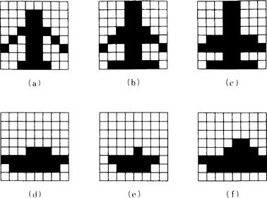
Suppose we have the six 8 × 8 bit input patterns shown in Figure 10.6. Suppose, of these patterns, (a)-(c) represent an airplane and (d)-(f) represent a ship. We will build a neural network for discriminating whether a given input pattern is an airplane or a ship using back propagation error learning.
Let us consider a neural network with feedforward links in three layers of 64 input units, 32 hidden units, and 2 output units. Links are connected from each input unit to all the hidden units and from each hidden unit to all the output units. Also, we assume that θj, the threshold value for each unit uj, can change, and we represent θj as the weight of a link from a special unit that always outputs 1 to uj. We also assume that the initial value of θj is 0 and set the initial value of the weights randomly between ±0.3.
The weights are updated using, as an example, a slightly different formula from the one described in Section 10.1:

In this example, the values of the coefficients are set to α = 0.80, η = 1.0. Also, the algorithm is supposed to terminate when the sum of the values of the evaluation function that are obtained when each of the six patterns is presented once is less than 0.06, i.e., when ![]() .
.
Using back propagation error learning with the six different input patterns in Figure 10.6 in the order (d), (a), (e), (b), (f), (c), the output converges in three cycles with the results shown in Figure 10.7. In other words, output unit u1 responds to the patterns of airplanes (a)-(c), and output unit u2 responds to the patterns of ships (d)-(e). ((a)-(f) are called the training patterns.)

If the two patterns (i) and (ii) (called test patterns) as shown in Figure 10.8(a) are input to the neural network obtained in this way, output unit u1 responds to (i) and u2 responds to (ii) as shown in Figure 10.8(b). Thus we can assume that (i) is an airplane and (ii) is a ship.

People are trying to apply back propagation error learning to visual pattern recognition, as shown here, to voice recognition, voice synthesis, expert systems, and so on.
10.3 Competitive Learning
One of the characteristics of the back propagation error learning algorithm described in Section 10.2 is that it is supervised learning. As opposed to this, competitive learning is known as unsupervised learning. Unsupervised learning is a method of learning without giving ideal output values (sometimes called teacher signals). In this section, we will explain neural networks and an algorithm for competitive learning.
(a) The structure of the neural network and an algorithm
First, we will explain neural networks where the units are clustered.
Let us look at a network with the structure shown in Figure 10.9. In other words, the input layer appears as the leftmost, the output layer appears as the rightmost, and each of them is a set of clusters including units. (Generally, clusters can either be overlapped or not overlapped, but in this section we consider neural networks where they do not overlap.) Between these layers, there is a certain number of hidden layers, and each layer is also made up of a certain number of clusters. In this section, we assume that there are no links connecting units in different clusters within one layer and that links do not exist between units in one cluster within the input or output cluster. Also, in any cluster in a hidden layer, any two units are connected with an inhibitory link. Furthermore, only excitatory links may exist between two units in clusters in neighboring layers from the input layer toward the output layer (see Figure 10.9).

With these conditions, let us consider neural networks with the following characteristics:
(1) At any one time, only one of the units in any cluster of a hidden layer produces output; the other units in the cluster do not. For example, consider a circuit where only the unit whose input size is the maximum will produce an output (a maximum-value detection circuit).
(2) It only updates the weights of the links that enter the units that produced the output in (1). (Section 10.3 (b) [example 7] shows a method different from this.)
Learning weights by giving output from only one unit in a cluster in a hidden layer or the output layer within a clustered network as described above is called competitive learning since the output result is obtained by a competition among units within each cluster.
Next, let us look at an algorithm for competitive learning. Consider the following algorithm for the neural networks shown in Figure 10.9.
Algorithm 10.3
[1] Let wji be the weight of an excitatory link from unit i to unit j, where Σi wji = 1. Then, based on

wji is changed by setting wji = wji + αΔwji, where nk is the number of input units that give outputs for the kth input pattern, α and γ are positive constants, and

Let us consider a convergent state in the above algorithm, that is, an equilibrium state where the input and output values are equal for any unit. In this case, the link weight wji is in proportion to the conditional probability that the link from unit i to j is activated when unit j is responding. Let us prove this. Let pk be the probability that the kth input pattern is given, and let vjk be the probability that unit j responds to the kth input pattern. Then, from (10.15),
Since the value of (10.16) is 0 in an equilibrium state, we have
Therefore

Now, let us assume that the sizes of input patterns are the same. In other words, we assume nk = n for any k. Then, (10.17) becomes
(10.18) shows that the weight of a link in an equilibrium state, wji, is in proportion to the conditional probability that the link from i to j is activated when j is responding.
We can say that, when the above algorithm reaches an equilibrium state, the network responds to similar input patterns more strongly and to non-similar input patterns more weakly. Let us prove this.
Suppose a new lth input pattern is given in the equilibrium state, and let ijl be the input to unit j. Then we have

If we set
we have
We can consider that (10.19) is the number of links that are activated for both the kth and lth input patterns, and it shows the similarity between the kth and lth input patterns. Therefore (10.20) shows that unit j; in an equilibrium state, responds more strongly to a similar input pattern and more weakly to an input pattern that is not so similar.
From these remarks an equilibrium state that can be reached using competitive learning by Algorithm 10.3 has some significance in processing similar patterns. Actually which equilibrium state can be reached is constrained depending on how output is chosen at each cluster. For example, if we use the maximum-value detection circuit, even when the equilibrium state mentioned above is reached, it has the following constraint:

(b) An example of competitive learning
[Example 6]
A method of pattern classification
Suppose we have a carrot, an apple, a cucumber, a kiwi, an eggplant, and grapes as objects, and they are given as the 13-bit patterns shown in Figure 10.10. Each bit in these patterns shows the color red, green, or purple and whether it is a vegetable or a fruit, where the color in a pattern can be slightly different due to differences in density.

Consider the two-layer network whose input layer consists of one cluster including 13 units and whose output layer consists of one cluster including two units and one cluster including three units. We assume there is no hidden layer. We set the parameters of (10.15), γ and α, to αγ = 1.0.
The patterns of Figure 10.10 are input in order once for each cycle and repeat for 100 cycles. The result is the output from the output clusters shown in Figure 10.11. The result for output cluster 1 shows that the six patterns are classified into {carrot, apple} and {cucumber, kiwi, eggplant, grapes}, in other words, red things and not red things. The result for output cluster 2 shows that they are classified into {kiwi, grapes} and {carrot, cucumber, eggplant}, {apple}, that is, green or purple fruits, vegetables, and red fruits.

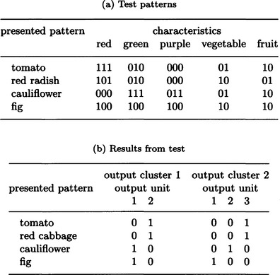
Next, the test patterns shown in Figure 10.12(a) are input to the network learned in this way, and we obtain the output shown in Figure 10.12(b). In other words, a tomato and a red radish are considered to be members of the red things when patterns are classified under two categories, and they are considered to be members of the red fruits when patterns are classified under three categories. Also, a cauliflower and a fig are considered to be green or purple fruits when patterns are classified into two categories, and a cauliflower is considered to be a vegetable and a fig is considered to be a green or purple vegetable when patterns are classified into three categories.
[Example 7]
There is a method that not only changes the weights of the links from the input units to units that have an output as in (10.15) but also changes the weights of the links connected to units that did not have an output. Although we did not say this in (a), the method uses the following formulas to change link weights:

Using the method of Example 6, the patterns in Figure 10.10 can be classified using both (10.21) and (10.15) by setting the parameters γ′ and α′ of (10.21) so that α′γ′ = 0.01. The results are shown in Figure 10.13(a).

The results show that the network can distinguish whether a pattern is a vegetable or a fruit when it classifies patterns into two classes and whether a pattern is red, green, or purple when it classifies patterns into three classes.
If we input the test patterns of Figure 10.12(a) to this trained network, we obtain the results shown in Figure 10.13(b). A tomato and a red radish are classified as vegetables when patterns are classified into two classes, and they are classified as red things when patterns are classified into three classes. Overall, a tomato and a red radish are classified as red vegetables. A cauliflower and a fig are classified as a green vegetable and a green fruit, respectively. Overall, we can say that they are classified as green things.
Pattern classification by competitive learning not only uses an unsupervised learning technique but also works without prior knowledge of classes to distinguish. In the above example, we gave the meanings such as vegetable, fruit, color, and so on. We did that for convenience. It does not mean that the patterns we used as examples correctly reflect the meanings that we gave them. However, the above example shows us that competitive learning can be used as a method for classifying patterns whose meaning is unknown.
10.4 Hopfield Networks
In a neural network where many units are linked to each other, if we limit the state of each unit to 0 or 1, we can represent the state of the whole network as a distribution pattern of local states each taking 0 or 1. In this global state, we can compare the state of each unit with the positive or negative direction of the spin of an electron using an analogy from physics. Under this comparison, if we let the potential of the global state of the network correspond to the energy of the spins, the thermodynamic process that tries to reach a state with the minimum spin energy corresponds to the process of finding an equilibrium state of the network.
Suppose we extend this idea and assume that the state of each unit can take a continuous value between [0, 1]. Then, if we consider the spin glass model* in physics, we can also make the energy function’s process of moving to a local minimum correspond to the neural network’s process of reaching an equilibrium state.
Based on this physical analogy, we can construct a neural network called a Hopfield network. In this section, we will explain Hopfield networks. Though the Hopfield network below is not basically a network for learning, it is explained here since it is a basic neural network representation and is deeply related to the Boltzmann machine that will be described in Section 10.5.
(a) The structure of the neural network and the algorithm
Let us look at the structure of a Hopfield network. Suppose we have a neural network where many units are interconnected with each other. The interconnection means that, if unit i is linked to j, then there is a link from j to i. We write aj(t) for the state of unit j at time t. Suppose aj(t) takes a value in [0, 1], and let ij(t) be the input to j and θj be the threshold value of j (note the sign of θ). If we let oi(t) be the output from unit i and wji the weight of the link from j to i, we have
We assume that the state of unit j, aj(t), changes according to the following rule:
Here τ is the time constant of the state of j. We assume the output of j is given by the following output function:
where a0 is a constant called the reference activation level.
Now, we define the energy of this neural network as follows:
If we assume wji = wij (symmetry of weights) for any i and j, we can bring the network to a local minimum value of E by computing the states of all units, aj(t), using (10.22), (10.23), and (10.24) repeatedly. The algorithm can be described simply as follows:
Algorithm 10.4
(minimization of the energy of a Hopfield network)
[1] Differentiate (10.23) and obtain the value of the difference Δt, the constant τ, and a0, the constant in (10.24).
[2] Set the values of the link weights wji and the threshold value θj.
[3] Update the states of all units repeatedly using (10.22), (10.23), and (10.24).
[4] When the value of E that is defined in (10.25) becomes smaller than some given positive constant, stop. (There are other stopping criteria.)
(b) Example of Hopfield networks
An optimization problem that minimizes an evaluation function under some constraints is frequently solved using mathematical programming. Optimization problems such as finding an optimal path in a graph generally include variables that take only discrete values. It becomes difficult to solve such a problem when it contains a large number of variables. A Hop-field network can be used for finding a locally optimal solution to this kind of problem.
[Example 8]
As an example, we will apply Hopfield networks to the traveling salesperson problem. The traveling salesperson problem is defined as the following optimization problem.
“Suppose there are n towns. Find the shortest route that starts at some town, visits every other town once and only once, and returns to the original town.”
Suppose the n towns are 1, …, n, and the distance between the towns i and j is dij. We define the variables

Then, the problem can be formalized as a problem of finding xij (i, j = 1, …, n) that minimize the following function. We let the state of each unit be 0 or 1. The following can be applied when the state of each unit takes a continuous value from [0, 1].

where A, B, and C are constants. The first term on the right side of (10.26) is the constraint that each town should be visited only once, the second term is the condition that the towns are visited one at a time, and the third term is to minimize the total distance. (10.26) assumes that there is no loop in any unit j. Let wi2j2,i1j1 be the weight of the link from (i1, j1) to (i2, j2)- Comparing (10.25) and (10.26) in the Hopfield network with n2 units that represents the fact that town i is visited at time j with the unit (i, j), the weight and the threshold value are

where

Then we can find a local minimum of E using Algorithm 10.4. A path that provides such value is a locally optimal solution to the original problem.
As an example, consider the 10 towns shown in Figure 10.14(a). These towns are the nodes of the strongly connected graph that allows movement between any two towns. The distance between towns is shown in Figure 10.14(a). For example, the distance between towns 5 and 8 is ![]() . Assume A = B = C = 1.0 and Δt = r = a0 = 1.0.
. Assume A = B = C = 1.0 and Δt = r = a0 = 1.0.

If we apply Algorithm 10.4 to this problem and its parameters, we get the result shown in Figure 10.14(b). The abscissa of the figure represents the name of a town and the ordinate represents the order of the visit on the route. The radius of the circle in the figure represents the state of the corresponding unit. The result in Figure 10.14(b) shows that, although there is still some noise, the route 10.14(c) starting from town 1 and going back to 1 was found by paying attention only to nodes whose radius is large.
10.5 Boltzmann Machines
As we said about the Hopfield network in Section 10.4, the behavior of some kinds of neural networks have the analog of a physical system moving toward a state of energy equilibrium. Under some conditions, the behavior of a neural network, where the input is given stochastically, can be described as statistical thermodynamic behavior. Using this analogy, by adding stochastic fluctuation to the state change of each unit, it is possible to make the energy a little bigger, and the network escapes from a local energy minimum and reaches the global minimum as shown in Figure 10.15.

Boltzmann machines are neural networks with this feature.
(a) Structure of the neural network and its algorithm
Let us consider a neural network that works in a stochastic environment in which the input data follow a given probability distribution. In this neural network, it is natural to assume that the state transition of each unit and its output also follow some probability distributions. Let us consider the following problem: how could we find the link weights of a network that makes its input-output relation have a probability distribution “as close as possible” to the probability distribution of the input-output data given from the outside?
Solving this problem corresponds to generalizing a Hopfield network to be stochastic. Below, we will describe an algorithm for solving the problem under some conditions. Algorithms of this kind, along with neural networks that compute them, are called Boltzmann machines. Unlike Hopfield networks, Boltzmann machines can learn link weights such that they minimize the error between the probability distribution of the ideal output and the distribution of actual output values.
First, we assume that in a neural network K with n units, the state sj of each unit j takes the value 0 or 1 stochastically. A state of K can be represented as an n-dimensional vector whose elements each stochastically take the value 0 or 1. We assume that for the weight of the link between units i and j, as in a Hopfield network, the symmetry wij = wji holds.
Now let us regard K as a statistical thermodynamic system consisting of n particles. If we let Eα be the energy of a state of K, α, the probability of K taking the state α is given by the Maxwell-Boltzmann distribution:
In (10.27), k is the Boltzmann constant. (When we consider K as a collection of particles that is in thermal equilibrium with an ideal gas having a large heat capacity, we can derive the above distribution using the idea of energy level.) T corresponds to temperature.
Corresponding to the energy function E defined in Section 10.4(a), we define energy Eα as follows:
Here we assume wij = wji, and ![]() and θj are the values of the state variable sj and the threshold in the state α, respectively.
and θj are the values of the state variable sj and the threshold in the state α, respectively.
The problem is now to find the weight that realizes the probability distribution of the input-output data “as precisely as possible” without any input from outside. For this, below we divide the set of the units of K into two groups, the set of the input and output units (visible units) A and the set of other units (hidden units) B. Let ![]() be the probability distribution for the state vector a of the set of visible units A, when there is no input and let α + β be the state vector of K for α and the state vector β of the set of the hidden units B. Then, similarly to (10.27), we have
be the probability distribution for the state vector a of the set of visible units A, when there is no input and let α + β be the state vector of K for α and the state vector β of the set of the hidden units B. Then, similarly to (10.27), we have
where Eαβ is the energy of K in the state α + β. If we let ![]() be the state of K in α + β, Eαβ is given, as before, by
be the state of K in α + β, Eαβ is given, as before, by
In the network described above, the probability distributions of the states of the input units and those of the output units are not separated. This kind of Boltzmann machine is called an autoassociative Boltzmann machine. On the other hand, the probability distribution of the states of the input units can be considered separately from the probability distribution of those of the output units when some input is given. Such a machine is called an mutually associative Boltzmann machine. We consider only the autoassociative Boltzmann machines.
From (10.30),
Thus, from (10.29),
When the input and output are given from outside of K, let ![]() be the probability distribution taken by α, the state vector of A. Since
be the probability distribution taken by α, the state vector of A. Since ![]() is determined only by the input and output, it is independent of wij. The problem here is to find that makes the difference between
is determined only by the input and output, it is independent of wij. The problem here is to find that makes the difference between ![]() and
and ![]() as small as possible. In order to do that, let us find wji. that makes the Kullback information measure for
as small as possible. In order to do that, let us find wji. that makes the Kullback information measure for ![]() and
and ![]()
a local minimum. If we differentiate G with respect to wij, we get the following using (10.31):
Now if, in an equilibrium, we assume that the probability of the state β of B when the state of A is fixed at a is equal to the probability of β when the state of A is not fixed, we have
However,

Therefore, from (10.33),
Also, for the probability ![]() ,
,
So, if we substitute (10.34) and (10.35) into (10.32), we get
where

Here, ![]() is the expected value of the probability distribution of the input-output data that makes the states of both units i and j 1 when K works by the input and output given from outside and reaches an equilibrium state. Similarly,
is the expected value of the probability distribution of the input-output data that makes the states of both units i and j 1 when K works by the input and output given from outside and reaches an equilibrium state. Similarly, ![]() can be interpreted as the expected value of an equilibrium state when there is no input from outside.
can be interpreted as the expected value of an equilibrium state when there is no input from outside.
(10.36) is the basic expression for obtaining an equilibrium state of the Boltzmann machine K, that is, the state where G takes a local minimum for wij. A characteristic of this expression is that it uses only information on units i and j to find the steepest descent direction of G for wij and does not require global information on K. (10.36) can be used for both input-output units and hidden units.
In (10.36), no method for determining the values of ![]() and
and ![]() is given. We will describe such a method below in (b). The
is given. We will describe such a method below in (b). The ![]() part, in other words, the part where the link between the neighboring units i and j is reinforced when both units are active, corresponds to the reinforcement learning mechanism of the Hebbian synapse proposed by Hebb. The
part, in other words, the part where the link between the neighboring units i and j is reinforced when both units are active, corresponds to the reinforcement learning mechanism of the Hebbian synapse proposed by Hebb. The ![]() part, in other words, the part where, in a situation with no input from outside, the link between the neighboring units i and j is weakened when they are both active, plays the role of preventing strange internal representations from being created automatically when K is working freely. That is, in (10.36),
part, in other words, the part where, in a situation with no input from outside, the link between the neighboring units i and j is weakened when they are both active, plays the role of preventing strange internal representations from being created automatically when K is working freely. That is, in (10.36), ![]() for making D work according to the input from the outside and
for making D work according to the input from the outside and ![]() for preventing K from working automatically according to the input when there is no input from outside resist one another.
for preventing K from working automatically according to the input when there is no input from outside resist one another.
(10.36) finds only one local minimum of G, but generally there can be many local minima. But if the state change of K is made stochastically and the size of this stochastic fluctuation is controlled by changing the value of the temperature T, K can move to the global minimum. We will describe this below.
(b) The heuristic method of learning
If the learning rule for a Boltzmann machine K, (10.36), can be computed, a (local) equilibrium state of K can be reached by determining the change of the weight wij using Δwij = −∂G/∂wij. To compute the learning rule (10.36), we need to find ![]() and
and ![]() and thus the products of the states of the two units,
and thus the products of the states of the two units, ![]() , and the probability distributions of the state vectors,
, and the probability distributions of the state vectors, ![]() These probability distributions are unknown and need to be determined statistically from some samples. To determine the changes of the weights, Δwij, effectively using the Boltzmann machine algorithm, we need to consider the following points:
These probability distributions are unknown and need to be determined statistically from some samples. To determine the changes of the weights, Δwij, effectively using the Boltzmann machine algorithm, we need to consider the following points:
In order to consider these points, we need to define the state transition function for each unit to change its state for a fixed value of T. This can be done by extending the state transition equation (10.23) in the Hopfield network to a stochastic one. For example, the energy gap, sj, between when the state of unit j takes the energy level 0 and when it takes the energy level 1 for the energy function E of the whole system is given by
Then the probability of a new state of unit j taking 1 is given by
Using (10.38), we can determine a new state of j probabilistically. Here, to determine ΔEj in (10.38), we need to know the current states of all the units, not just j as in (10.37). To do this in parallel is difficult in a system like a Boltzmann machine, where the state of each unit changes asynchronously; therefore, the value of pj can be determined only approximately in actual use.
We now consider how to determine the temperature, T. Note that (10.38) is the function illustrated in Figure 10.16 with T as a parameter. In other words, the smaller T is, the smaller the fluctuation of the probability pj becomes and it comes closer to a linear threshold function. If we set the value of T large in a place far from the global minimum of the energy function, the probability of getting out of a local minimum is large.
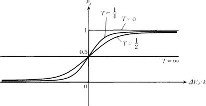
In a place near the global minimum, if we make the value of T small, we can obtain the minimum without going far from it. Changing the initially large value of T little by little to a smaller value during the process of energy minimization and state transition based on (10.38) is called annealing or simulated annealing.
There are many methods of annealing, such as
where t is the time or the number of iterations and ξ1, ξ2 are constants.
Let us consider how to determine ![]() and
and ![]() . For
. For ![]() , we can give the network the same input-output data many times, find the number of times that the states of units i and j are both 1, and assume that
, we can give the network the same input-output data many times, find the number of times that the states of units i and j are both 1, and assume that ![]() is that number. For
is that number. For ![]() , we do the same thing as for
, we do the same thing as for ![]() , but by fixing the state of each input unit to be 1, and assume that
, but by fixing the state of each input unit to be 1, and assume that ![]() is that number. For these T,
is that number. For these T, ![]() and
and ![]() , we update the weight of each link using
, we update the weight of each link using
where α and β are positive constants. The computation is terminated when the value of the energy function becomes smaller than a given criterion. In order to hasten the convergence, we could use heuristic methods rather than (10.39). Note that (10.39) and (10.40) are not the only possible method.
(c) Example of a Boltzmann machine
Unlike Hopfield networks, described in Section 10.4, in a Boltzmann machine it is possible to obtain the global minimum by giving probabilistic fluctuations to state transitions. By efficient annealing that changes the value of the temperature parameter T, it is possible to control the fluctuation effectively and increase the rate of convergence to the global minimum. By making use of this feature, we can use Boltzmann machines for solving optimization problems that include discrete variables. As we saw before, since the algorithm includes many assumptions unsatisfied in the actual computation on a computer, there is no guarantee that the algorithm always is able to attain the global minimum. In the example below, we obtain the minimum value of the energy function by probabilistic state transition and annealing by keeping the link weights fixed rather than learning them as in (10.39) and (10.40).
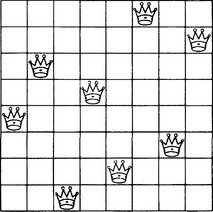
Let us consider the n-queen problem as an example of an optimization problem.
‘Place n queens on an n x n chessboard so that no queens can capture each other in the vertical, horizontal, or diagonal direction.‘
Figure 10.17 shows one solution to the eight-queen problem.
To solve the n-queen problem, we regard each square on the board as a unit and consider the neural network where all the units are linked to each other. Let (i, j) be the square on the ith row and the jth column. Now, using the variables
we define the evaluation function of the problem as follows:

The first, second, third, and fourth terms on the right side correspond to the conditions that only one queen exists on each row, column, and diagonal line from the upper right to the lower left or from the upper left to the lower right, respectively.
Then, if we make (10.41) correspond to the energy function (10.28), we have

where wi1jl,i2j2 is the weight of the link from unit (i2, j2) to (i1, j1), and θij is the threshold value of unit (i, j).
Next, using (10.42), (10.43) and (10.37), (10.38), we obtain the probability pj that the state of unit j moves to 1, where we set A = B = C = D = 10.0 and define the schedule of annealing by
To do the computation, we set T0 = 25.0, τ = 4.0. Then, starting from iteration t = 0, we obtain pj for all the units at each iteration. Every time we obtain pj n2 times, we increase t by 1 and then decrease the size of T using (10.44).
In this way, as we probabilistically change the next state to 1 by using Pj obtained at each iteration, we can make the value of the energy function smaller. In the case of (10.41), E = 0 at the global minimum.
When we apply this method to the eight-queen problem (n = 8), we obtain E ≈ 0 at t = 49 and obtain the result shown in Figure 10.18(a). In the 100-queen problem (n = 100), E ≈ 0 is attained at t = 111, and we obtain the result shown in Figure 10.18(b).

10.6 Parallel Computation in Recognition and Learning
The Hopfield network and the Boltzmann machine start from an initial value that may not satisfy any constraints and reach a state that satisfies local constraints on the links between the units. This is a relaxation method. In the computation of the neural network using the relaxation method, we may not always obtain a solution that perfectly satisfies all the constraints. In other words, the computation of the neural network can be considered a weak relaxation method.
The weak relaxation method not only is used in the neural networks described in this chapter but also can be used in models based on other algorithms that use slightly different locally parallel computations. For example, it can be used in a restoration algorithm for a visual pattern based on the concept of a Markov process.
Suppose f is a pattern function that is defined on a set D of a finite number of pattern elements. Assume that the pattern, including noises and defects, appears as a sample from a probabilistic pattern representation. In order to represent this formally, we, for example, assume that a random probability variable Xd corresponds to the element of each pattern d ∈ D and consider the probability distribution on D as a whole, X = {Xd|d ∈ D}.
On the other hand, we assume that the probabilistic value of Xd for some pattern element d is determined not by the whole probability distribution but only by a neighborhood of d. To express this formally, we can do the following: First, assume that the neighborhood of a random d ∈ D, Nd, is defined, where if d′ ∈ Nd, then d ∈ Nd′. For example, when d is a pixel in a two-dimensional visual pattern, we refer to the set of the pixels that are neighbors of d as Nd- Furthermore, let II be the simultaneous probability distribution function of Nd for all Xd. Using these definitions, we assume the probability of Xd taking the value h is only on {Xd’d′ ∈ Nd}. In other words, we assume
When this assumption is true, we say that X is a Markov process.
Given a Markov process, under appropriate conditions, we can restore the original pattern function from a sample of the pattern function that includes noise by minimizing some local energy function that can be computed from the simultaneous probability distribution function of each neighbor. Its principle is beyond the scope of this book, so we will not describe it. However, the fact the original pattern can be restored by doing parallel computation on each neighborhood of each pattern element means that we can remove noise by doing many local computations in parallel.
Furthermore, we can use the method of probabilistic state transition to minimize the energy function. Also, while in the Boltzmann machine the equilibrium state is limited to the Maxwell-Boltzmann distribution and expression (10.38) is used for the state transition, recent study begins to show that a weak relaxation method similar to the Boltzmann machine can be used for a wider collection of probability distributions.
What we have described is simply one example to show that a neural network is an example of an algorithm that makes use of massively parallel computation that is beginning to be used in pattern information processing. We consider massively parallel computation as a parallel computation using an architecture that closely links many tens of thousands of processors. Due to improvements in hardware technology, we are able to use computation methods like this to process massive data at high speeds, and algorithms for massively parallel computation become important. Also, massively parallel computation is used not only in numeric processing, as in neural networks and algorithms for pattern information processing, but also in inferences based on symbol representation and learning. In this book, we could not cover parallel processing algorithms; however, many algorithms in the area of massively parallel computation will be developed during research on pattern recognition and learning that requires the high-speed processing of massive amounts of data. Such development will play a central role in improving the capability of software that benefits human beings.
Summary
In this chapter, we described methods for learning pattern discrimination, pattern classification, optimization, and so on, using neural networks.
10.1. A neural network is a dynamic network representation that can be defined by giving its nodes (called units), directed edges (called links), the weight of each link, the state transition functions, and the output functions of the units.
10.2. A simple three-layer perceptron is a kind of neural network that can discriminate linearly separable patterns.
10.3. Back propagation error learning is supervised learning in a neural network that is structured as a feedforward graph, and it can be used to obtain a neural network that makes the square sum of the differences between the ideal output values and the actual output values a local minimum.
10.4. Competitive learning is unsupervised learning in a neural network that has clustered units. It can learn to do pattern classification by competition among the units included in each cluster.
10.5. A Hopfield network is an algorithm for a neural network with mutually linked units where the state of each unit takes a continuous value between [0,1] that computes states so that its energy function takes a local minimum.
10.6. A Boltzmann machine is an algorithm for obtaining the global minimum of the energy function by introducing stochastic fluctuation to the state transitions in a Hopfield network.
10.7. Using an annealing method that decreases, based on appropriate rules, the value of the parameter that corresponds to thermodynamic temperature, we can increase the rate of convergence to the global minimum.
10.8. High-speed processing of massive data is necessary for problems concerned with pattern recognition and learning. Algorithms that allow massively parallel computation such as the relaxation method are important for these problems.
Exercises
(i) List the major differences between back propagation error learning and competitive learning.
(ii) List the major differences between a Hopfield network and a Boltzmann machine.
10.2. We assume, in a neural network consisting of an input layer and an output layer, that every input unit has a link to all the output units. We also assume that the output layer consists of units lined up in a two-dimensional array. For this network, let xj(t) be the input to j at time t and wjh(t) be the weight of the link from input unit j to output unit k. Let us denote the neighborhood of the output unit k at time t as N(k, t) and assume that N(k, t1) ⊂ N(k, t2) holds for any times t1, t2 satisfying t1 < t2 (usually, we use the set of the m2 units included in an m ∧ m square whose center is k). Now, let us consider the following:
[1] Set the weight wkj of all the links to a small random value.
[2] Set t = 0. Define N(k, 0) for all the output units k. (N(k, 0) can be, for example, a large square with k as a center.) Let α(0) be a function satisfying 0 < α(0) < 1.
[3] Stop when there is no datum at time t + 1. Otherwise, input the datum for time t + 1.
for all output units k.
[6] For all output units k ∈ N(k*, t), set
for each input unit j.
[7] Define α(t + 1) satisfying α(t + 1) < α(t).Set t = t + 1 and go to [4].
Explain what kind of processing this algorithm does. (This algorithm is called a self-organizing feature map.)
10.3. List the functions necessary for a neural network description language.
*That a real-valued function f(x) defined on n-dimensional Euclidean space En takes a local minimum at a point x* means that there exists ∈ > 0 such that, for the ∈-neighborhood of x*, N(x*, ∈) ⊆ En, f(x*) ≤ f(x) for all x ∈ N(x*, ∈). When f(x*) ≤ f(x) for all x ∈ En, we say that f(x) has a global minimum at x*. When f(x) is differentiate, ![]() is the direction where the value of f(x) at
is the direction where the value of f(x) at ![]() is decreasing the fastest. This direction is called the steepest descent direction of f(x) at
is decreasing the fastest. This direction is called the steepest descent direction of f(x) at ![]() , and the method for obtaining a local minimum of f(x) by successively obtaining the steepest descent direction is called the steepest descent method.
, and the method for obtaining a local minimum of f(x) by successively obtaining the steepest descent direction is called the steepest descent method.
*An irregular magnetic substance whose magnetic interaction can be positive or negative and that has the order phase without long-distance order under a certain temperature is called spin glass. Under such a temperature, it is considered that there exist numerous semistable states that move gradually toward stable states as the temperature is reduced.