A Small Example: Predicting Loan Default

Table 6-1 shows a few records of personal loan data from the Lending Club. Lending Club is a leader in peer-to-peer lending in which pools of investors make personal loans to individuals. The goal of an analysis would be to predict the outcome of a new potential loan: paid-off versus default.

Consider a very simple model with just two predictor variables: dti, which is the ratio of debt payments (excluding mortgage) to income, and payment_inc_ratio, which is the ratio of the loan payment to income. Both ratios are multiplied by 100. Using a small set of 200 loans, loan200, with known binary outcomes (default or no-default, specified in the predictor outcome200), and with K set to 20, the KNN estimate for a new loan to be predicted, newloan, with dti=22.5 and payment_inc_ratio=9 can be calculated in R as follows:

newloan <- loan200[1, 2:3, drop=FALSE]
knn_pred <- knn(train=loan200[-1,2:3], test=newloan, cl=loan200[-1,1], k=20)
knn_pred == 'paid off'
[1] TRUE

The KNN prediction is for the loan to default.

While R has a native knn function, the contributed R package FNN, for Fast Nearest Neighbor, scales to big data better and provides more flexibility.

Figure 6-2 gives a visual display of this example. The new loan to be predicted is the square in the middle. The circles (default) and crosses (paid off) are the training data. The black line shows the boundary of the nearest 20 points. In this case, 9 defaulted loans lie within the circle as compared with 11 paid-off loans. Hence the predicted outcome of the loan is paid-off.

Figure 6-2. KNN prediction of loan default using two variables: debt-to-income ratio and loan payment-to-income ratio

Distance Metrics

Similarity (nearness) is determined using a distance metric, which is a function that measures how far two records (x₁, x₂, … x_p) and (u₁, u₂, … u_p) are from one another. The most popular distance metric between two vectors is Euclidean distance. To measure the Euclidean distance between two vectors, subtract one from the other, square the differences, sum them, and take the square root:

Euclidean distance offers special computational advantages. This is particularly important for large data sets since KNN involves K × n pairwise comparisons where n is the number of rows.

Another common distance metric for numeric data is Manhattan distance:

Euclidean distance corresponds to the straight-line distance between two points (e.g., as the crow flies). Manhattan distance is the distance between two points traversed in a single direction at a time (e.g., traveling along rectangular city blocks). For this reason, Manhattan distance is a useful approximation if similarity is defined as point-to-point travel time.

In measuring distance between two vectors, variables (features) that are measured with comparatively large scale will dominate the measure. For example, for the loan data, the distance would be almost solely a function of the income and loan amount variables, which are measured in tens or hundreds of thousands. Ratio variables would count for practically nothing in comparison. We address this problem by standardizing the data; see “Standardization (Normalization, Z-Scores)”.

One Hot Encoder

The loan data in Table 6-1 includes several factor (string) variables. Most statistical and machine learning models require this type of variable to be converted to a series of binary dummy variables conveying the same information, as in Table 6-2. Instead of a single variable denoting the home occupant status as “owns with a mortage,” “owns with no mortgage,” “rents,” or “other,” we end up with four binary variables. The first would be “owns with a mortgage—Y/N,” the second would be “owns with no mortgage—Y/N,” and so on. This one predictor, home occupant status, thus yields a vector with one 1 and three 0s, that can be used in statistical and machine learning algorithms. The phrase one hot encoding comes from digital circuit terminology, where it describes circuit settings in which only one bit is allowed to be positive (hot).

Standardization (Normalization, Z-Scores)

In measurement, we are often not so much interested in “how much” but “how different from the average.” Standardization, also called normalization, puts all variables on similar scales by subtracting the mean and dividing by the standard deviation. In this way, we ensure that a variable does not overly influence a model simply due to the scale of its original measurement.

These are commonly refered to as z-scores. Measurements are then stated in terms of “standard deviations away from the mean.” In this way, a variable’s impact on a model is not affected by the scale of its original measurement.

For KNN and a few other procedures (e.g., principal components analysis and clustering), it is essential to consider standardizing the data prior to applying the procedure. To illustrate this idea, KNN is applied to the loan data using dti and payment_inc_ratio (see “A Small Example: Predicting Loan Default”) plus two other variables: revol_bal, the total revolving credit available to the applicant in dollars, and revol_util, the percent of the credit being used. The new record to be predicted is shown here:

newloan
  payment_inc_ratio dti revol_bal revol_util
1            2.3932   1      1687        9.4

The magnitude of revol_bal, which is in dollars, is much bigger than the other variables. The knn function returns the index of the nearest neighbors as an attribute nn.index, and this can be used to show the top-five closest rows in loan_df:

loan_df <- model.matrix(~ -1 + payment_inc_ratio + dti + revol_bal +
                           revol_util, data=loan_data)
newloan = loan_df[1,, drop=FALSE]
loan_df = loan_df[-1,]
outcome <- loan_data[-1,1]
knn_pred <- knn(train=loan_df, test=newloan, cl=outcome, k=5)
loan_df[attr(knn_pred,"nn.index"),]

        payment_inc_ratio  dti revol_bal revol_util
35537             1.47212 1.46      1686       10.0
33652             3.38178 6.37      1688        8.4
25864             2.36303 1.39      1691        3.5
42954             1.28160 7.14      1684        3.9
43600             4.12244 8.98      1684        7.2

The value of revol_bal in these neighbors is very close to its value in the new record, but the other predictor variables are all over the map and essentially play no role in determining neighbors.

Compare this to KNN applied to the standardized data using the R function scale, which computes the z-score for each variable:

loan_df <- model.matrix(~ -1 + payment_inc_ratio + dti + revol_bal +
                           revol_util, data=loan_data)
loan_std <- scale(loan_df)
target_std = loan_std[1,, drop=FALSE]
loan_std = loan_std[-1,]
outcome <- loan_data[-1,1]
knn_pred <- knn(train=loan_std, test=target_std, cl=outcome, k=5)
loan_df[attr(knn_pred,"nn.index"),]
        payment_inc_ratio   dti  revol_bal  revol_util
2080            10.04400  19.89       9179        51.5
1438            3.87890    5.31       1687        51.1
30215           6.71820   15.44       4295        26.0
28542           6.93816   20.31      11182        76.1
44737           8.20170   16.65       5244        73.9

The five nearest neighbors are much more alike in all the variables providing a more sensible result. Note that the results are displayed on the original scale, but KNN was applied to the scaled data and the new loan to be predicted.

Choosing K

The choice of K is very important to the performance of KNN. The simplest choice is to set $K=1$, known as the 1-nearest neighbor classifier. The prediction is intuitive: it is based on finding the data record in the training set most similar to the new record to be predicted. Setting $K=1$ is rarely the best choice; you’ll almost always obtain superior performance by using K > 1-nearest neighbors.

Generally speaking, if K is too low, we may be overfitting: including the noise in the data. Higher values of K provide smoothing that reduces the risk of overfitting in the training data. On the other hand, if K is too high, we may oversmooth the data and miss out on KNN’s ability to capture the local structure in the data, one of its main advantages.

The K that best balances between overfitting and oversmoothing is typically determined by accuracy metrics and, in particular, accuracy with holdout or validation data. There is no general rule about the best K—it depends greatly on the nature of the data. For highly structured data with little noise, smaller values of K work best. Borrowing a term from the signal processing community, this type of data is sometimes referred to as having a high signal-to-noise ratio (SNR). Examples of data with typically high SNR are handwriting and speech recognition. For noisy data with less structure (data with a low SNR), such as the loan data, larger values of K are appropriate. Typically, values of K fall in the range 1 to 20. Often, an odd number is chosen to avoid ties.

KNN as a Feature Engine

KNN gained its popularity due to its simplicity and intuitive nature. In terms of performance, KNN by itself is usually not competitive with more sophisticated classification techniques. In practical model fitting, however, KNN can be used to add “local knowledge” in a staged process with other classification techniques.

1. KNN is run on the data, and for each record, a classification (or quasi-probability of a class) is derived.

2. That result is added as a new feature to the record, and another classification method is then run on the data. The original predictor variables are thus used twice.

At first you might wonder whether this process, since it uses some predictors twice, causes a problem with multicollinearity (see “Multicollinearity”). This is not an issue, since the information being incorporated into the second-stage model is highly local, derived only from a few nearby records, and is therefore additional information, and not redundant.

For example, consider the King County housing data. In pricing a home for sale, a realtor will base the price on similar homes recently sold, known as “comps.” In essence, realtors are doing a manual version of KNN: by looking at the sale prices of similar homes, they can estimate what a home will sell for. We can create a new feature for a statistical model to mimic the real estate professional by applying KNN to recent sales. The predicted value is the sales price and the existing predictor variables could include location, total square feet, type of structure, lot size, and number of bedrooms and bathrooms. The new predictor variable (feature) that we add via KNN is the KNN predictor for each record (analogous to the realtors’ comps). Since we are predicting a numerical value, the average of the K-Nearest Neighbors is used instead of a majority vote (known as KNN regression).

Similarly, for the loan data, we can create features that represent different aspects of the loan process. For example, the following would build a feature that represents a borrower’s creditworthiness:

borrow_df <- model.matrix(~ -1 + dti + revol_bal + revol_util + open_acc +
                            delinq_2yrs_zero + pub_rec_zero, data=loan_data)
borrow_knn <- knn(borrow_df, test=borrow_df, cl=loan_data[, 'outcome'],
                  prob=TRUE, k=20)
prob <- attr(borrow_knn, "prob")
borrow_feature <- ifelse(borrow_knn=='default', 1-prob, prob)
summary(borrow_feature)
   Min.  1st Qu.  Median    Mean   3rd Qu.  Max.
  0.050    0.400   0.500   0.499    0.600  1.000

The result is a feature that predicts the likelihood a borrower will default based on his credit history.

A Simple Example

The two main packages to fit tree models in R are rpart and tree. Using the rpart package, a model is fit to a sample of 3,000 records of the loan data using the variables payment_inc_ratio and borrower_score (see “K-Nearest Neighbors” for a description of the data).

library(rpart)
loan_tree <- rpart(outcome ~ borrower_score + payment_inc_ratio,
                   data=loan_data, control = rpart.control(cp=.005))
plot(loan_tree, uniform=TRUE, margin=.05)
text(loan_tree)

The resulting tree is shown in Figure 6-3. These classification rules are determined by traversing through a hierarchical tree, starting at the root and moving left if the node is true and right if not, until a leaf is reached.

Typically, the tree is plotted upside-down, so the root is at the top and the leaves are at the bottom. For example, if we get a loan with borrower_score of 0.6 and a payment_inc_ratio of 8.0, we end up at the leftmost leaf and predict the loan will be paid off.

Figure 6-3. The rules for a simple tree model fit to the loan data

A nicely printed version of the tree is also easily produced:

loan_tree
n= 3000

node), split, n, loss, yval, (yprob)
    * denotes terminal node

1) root 3000 1445 paid off (0.5183333 0.4816667)
  2) borrower_score>=0.575 878  261 paid off (0.7027335 0.2972665) *
  3) borrower_score< 0.575 2122  938 default (0.4420358 0.5579642)
    6) borrower_score>=0.375 1639  802 default (0.4893228 0.5106772)
      12) payment_inc_ratio< 10.42265 1157  547 paid off (0.5272256 0.4727744)
        24) payment_inc_ratio< 4.42601 334  139 paid off (0.5838323 0.4161677) *
        25) payment_inc_ratio>=4.42601 823  408 paid off (0.5042527 0.4957473)
          50) borrower_score>=0.475 418  190 paid off (0.5454545 0.4545455) *
          51) borrower_score< 0.475 405  187 default (0.4617284 0.5382716) *
      13) payment_inc_ratio>=10.42265 482  192 default (0.3983402 0.6016598) *
    7) borrower_score< 0.375 483  136 default (0.2815735 0.7184265) *

The depth of the tree is shown by the indent. Each node corresponds to a provisional classification determined by the prevalent outcome in that partition. The “loss” is the number of misclassifications yielded by the provisional classification in a partition. For example, in node 2, there were 474 misclassification out of a total of 1,467 total records. The values in the parentheses correspond to the proportion of records that are paid off and default, respectively. For example, in node 13, which predicts default, over 60 percent of the records are loans that are in default.

The Recursive Partitioning Algorithm

The algorithm to construct a decision tree, called recursive partitioning , is straightforward and intuitive. The data is repeatedly partitioned using predictor values that do the best job of separating the data into relatively homogeneous partitions. Figure 6-4 shows the partitions created for the tree in Figure 6-3. The first rule is borrower_score >= 0.575 and is depicted by rule 1 in the plot and segments the right portion. The second rule is borrower_score < 0.375 and segments the left portion.

Figure 6-4. The first three rules for a simple tree model fit to the loan data

Suppose we have a response variable Y and a set of P predictor variables X_j for $j=1,\cdots ,P$. For a partition A of records, recursive partitioning will find the best way to partition A into two subpartitions:

1. For each predictor variable X_j,

   1. For each value s_j of X_j:

      1. Split the records in A with X_j values < s_j as one partition, and the remaining records where X_j ≥ s_j as another partition.

      2. Measure the homogeneity of classes within each subpartition of A.

   2. Select the value of s_j that produces maximum within-partition homogeneity of class.

2. Select the variable X_j and the split value s_j that produces maximum within-partition homogeneity of class.

Now comes the recursive part:

1. Initialize A with the entire data set.

2. Apply the partitioning algorithm to split A into two subpartitions, A₁ and A₂.

3. Repeat step 2 on subpartitions A₁ and A₂.

4. The algorithm terminates when no further partition can be made that sufficiently improves the homogeneity of the partitions.

The end result is a partitioning of the data, as in Figure 6-4 except in P-dimensions, with each partition predicting an outcome of 0 or 1 depending on the majority vote of the reponse in that partition.

Measuring Homogeneity or Impurity

Tree models recursively create partitions (sets of records), A, that predict an outcome of Y = 0 or Y = 1. You can see from the preceding algorithm that we need a way to measure homogeneity, also called class purity, within a partition. Or, equivalently, we need to measure the impurity of a partition. The accuracy of the predictions is the proportion p of misclassified records within that partition, which ranges from 0 (perfect) to 0.5 (purely random guessing).

It turns out that accuracy is not a good measure for impurity. Instead, two common measures for impurity are the Gini impurity and entropy of information. While these (and other) impurity measures apply to classification problems with more than two classes, we focus on the binary case. The Gini impurity for a set of records A is:

The entropy measure is given by:

Figure 6-5 shows that Gini impurity (rescaled) and entropy measures are similar, with entropy giving higher impurity scores for moderate and high accuracy rates.

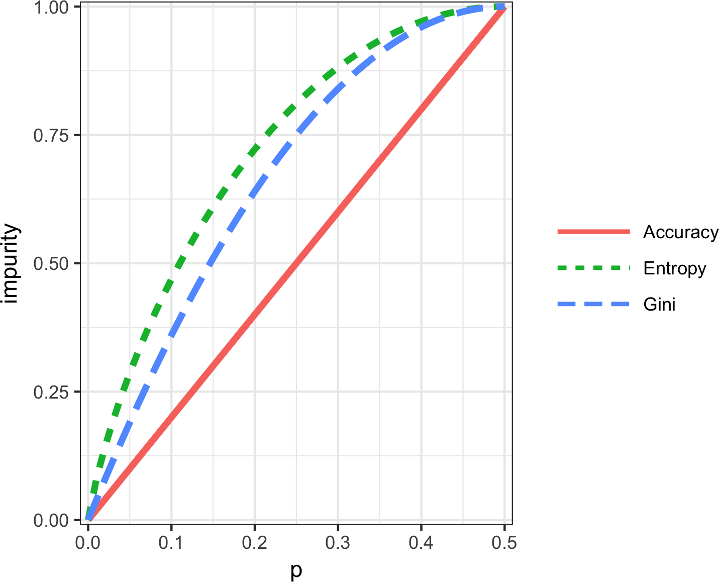
Figure 6-5. Gini impurity and entropy measures

The impurity metric is used in the splitting algorithm described earlier. For each proposed partition of the data, impurity is measured for each of the partitions that result from the split. A weighted average is then calculated, and whichever partition (at each stage) yields the lowest weighted average is selected.

Stopping the Tree from Growing

As the tree grows bigger, the splitting rules become more detailed, and the tree gradually shifts from identifying “big” rules that identify real and reliable relationships in the data to “tiny” rules that reflect only noise. A fully grown tree results in completely pure leaves and, hence, 100% accuracy in classifying the data that it is trained on. This accuracy is, of course, illusory—we have overfit (see Bias-Variance Tradeoff) the data, fitting the noise in the training data, not the signal that we want to identify in new data.

We need some way to determine when to stop growing a tree at a stage that will generalize to new data. There are two common ways to stop splitting:

• Avoid splitting a partition if a resulting subpartition is too small, or if a terminal leaf is too small. In rpart, these constraints are controlled separately by the parameters minsplit and minbucket, respectively, with defaults of 20 and 7.

• Don’t split a partition if the new partition does not “significantly” reduce the impurity. In rpart, this is controlled by the complexity parameter cp, which is a measure of how complex a tree is—the more complex, the greater the value of cp. In practice, cp is used to limit tree growth by attaching a penalty to additional complexity (splits) in a tree.

The first method involves arbitrary rules, and can be usful for exploratory work, but we can’t easily determine optimum values (i.e., values that maximize predictive accuracy with new data). With the complexity parameter, cp, we can estimate what size tree will perform best with new data.

If cp is too small, then the tree will overfit the data, fitting noise and not signal. On the other hand, if cp is too large, then the tree will be too small and have little predictive power. The default in rpart is 0.01, although for larger data sets, you are likely to find this is too large. In the previous example, cp was set to 0.005 since the default led to a tree with a single split. In exploratory analysis, it is sufficient to simply try a few values.

Determining the optimum cp is an instance of the bias-variance tradeoff (see Bias-Variance Tradeoff). The most common way to estimate a good value of cp is via cross-validation (see “Cross-Validation”):

1. Partition the data into training and validation (holdout) sets.

2. Grow the tree with the training data.

3. Prune it successively, step by step, recording cp (using the training data) at each step.

4. Note the cp that corresponds to the minimum error (loss) on the validation data.

5. Repartition the data into training and validation, and repeat the growing, pruning, and cp recording process.

6. Do this again and again, and average the cps that reflect minimum error for each tree.

7. Go back to the original data, or future data, and grow a tree, stopping at this optimum cp value.

In rpart, you can use the argument cptable to produce a table of the cp values and their associated cross-validation error (xerror in R), from which you can determine the cp value that has the lowest cross-validation error.

Predicting a Continuous Value

Predicting a continuous value (also termed regression) with a tree follows the same logic and procedure, except that impurity is measured by squared deviations from the mean (squared errors) in each subpartition, and predictive performance is judged by the square root of the mean squared error (RMSE) (see “Assessing the Model”) in each partition.

How Trees Are Used

One of the big obstacles faced by predictive modelers in organizations is the perceived “black box” nature of the methods they use, which gives rise to opposition from other elements of the organization. In this regard, the tree model has two appealing aspects.

• Tree models provide a visual tool for exploring the data, to gain an idea of what variables are important and how they relate to one another. Trees can capture nonlinear relationships among predictor variables.

• Tree models provide a set of rules that can be effectively communicated to nonspecialists, either for implementation or to “sell” a data mining project.

When it comes to prediction, however, harnassing the results from multiple trees is typically more powerful than just using a single tree. In particular, the random forest and boosted tree algorithms almost always provide superior predictive accuracy and performance (see “Bagging and the Random Forest” and “Boosting”), but the aforementioned advantages of a single tree are lost.

Further Reading

• Analytics Vidhya Content Team, “A Complete Tutorial on Tree Based Modeling from Scratch (in R & Python)”, April 12, 2016.

• Terry M. Therneau, Elizabeth J. Atkinson, and the Mayo Foundation, “An Introduction to Recursive Partitioning Using the RPART Routines”, June 29, 2015.

Bagging

Bagging, which stands for “bootstrap aggregating,” was introduced by Leo Breiman in 1994. Suppose we have a response Y and P predictor variables $?=X_1,X_2,\cdots ,X_P$ with N records.

Bagging is like the basic algorithm for ensembles, except that, instead of fitting the various models to the same data, each new model is fit to a bootstrap resample. Here is the algorithm presented more formally:

1. Initialize M, the number of models to be fit, and n, the number of records to choose (n < N). Set the iteration $m=1$.

2. Take a bootstrap resample (i.e., with replacement) of n records from the training data to form a subsample $Y_m$ and ${?}_m$ (the bag).

3. Train a model using $Y_m$ and ${?}_m$ to create a set of decision rules ${\widehat{f}}_m\left(?\right)$.

4. Increment the model counter $m=m+1$. If m <= M, go to step 1.

In the case where ${\widehat{f}}_m$ predicts the probability $Y=1$, the bagged estimate is given by:

Random Forest

The random forest is based on applying bagging to decision trees with one important extension: in addition to sampling the records, the algorithm also samples the variables.³ In traditional decision trees, to determine how to create a subpartition of a partition A, the algorithm makes the choice of variable and split point by minimizing a criterion such as Gini impurity (see “Measuring Homogeneity or Impurity”). With random forests, at each stage of the algorithm, the choice of variable is limited to a random subset of variables. Compared to the basic tree algorithm (see “The Recursive Partitioning Algorithm”), the random forest algorithm adds two more steps: the bagging discussed earlier (see “Bagging and the Random Forest”), and the bootstrap sampling of variables at each split:

1. Take a bootstrap (with replacement) subsample from the records.

2. For the first split, sample p < P variables at random without replacement.

3. For each of the sampled variables $X_{j\left(1\right)},X_{j\left(2\right)},...,X_{j\left(p\right)}$, apply the splitting algorithm:

   1. For each value $s_{j\left(k\right)}$ of $X_{j\left(k\right)}$:

      1. Split the records in partition A with X_j(k) < s_j(k) as one partition, and the remaining records where $X_{j\left(k\right)}\ge s_{j\left(k\right)}$ as another partition.

      2. Measure the homogeneity of classes within each subpartition of A.

   2. Select the value of $s_{j\left(k\right)}$ that produces maximum within-partition homogeneity of class.

4. Select the variable $X_{j\left(k\right)}$ and the split value $s_{j\left(k\right)}$ that produces maximum within-partition homogeneity of class.

5. Proceed to the next split and repeat the previous steps, starting with step 2.

6. Continue with additional splits following the same procedure until the tree is grown.

7. Go back to step 1, take another bootstrap subsample, and start the process over again.

How many variables to sample at each step? A rule of thumb is to choose $\sqrt{P}$ where P is the number of predictor variables. The package randomForest implements the random forest in R. The following applies this package to the loan data (see “K-Nearest Neighbors” for a description of the data).

rf <- randomForest(outcome ~ borrower_score + payment_inc_ratio,
                    data=loan3000)
rf

Call:
 randomForest(formula = outcome ~ borrower_score + payment_inc_ratio,
     data = loan3000)
           	Type of random forest: classification
                     Number of trees: 500
No. of variables tried at each split: 1

    	OOB estimate of  error rate: 39.17%
Confusion matrix:
        default  paid off  class.error
default     873       572   0.39584775
paid off    603       952   0.38778135

By default, 500 trees are trained. Since there are only two variables in the predictor set, the algorithm randomly selects the variable on which to split at each stage (i.e., a bootstrap subsample of size 1).

The out-of-bag (OOB) estimate of error is the error rate for the trained models, applied to the data left out of the training set for that tree. Using the output from the model, the OOB error can be plotted versus the number of trees in the random forest:

error_df = data.frame(error_rate = rf$err.rate[,'OOB'],
                      num_trees = 1:rf$ntree)
ggplot(error_df, aes(x=num_trees, y=error_rate)) +
  geom_line()

The result is shown in Figure 6-6. The error rate rapidly decreases from over .44 before stabilizing around .385. The predicted values can be obtained from the predict function and plotted as follows:

pred <- predict(rf, prob=TRUE)
rf_df <- cbind(loan3000, pred = pred)
ggplot(data=rf_df, aes(x=borrower_score, y=payment_inc_ratio,
                       shape=pred, color=pred)) +
  geom_point(alpha=.6, size=2) +
  scale_shape_manual( values=c( 46, 4))

Figure 6-6. The improvement in accuracy of the random forest with the addition of more trees

The plot, shown in Figure 6-7, is quite revealing about the nature of the random forest.

Figure 6-7. The predicted outcomes from the random forest applied to the loan default data

The random forest method is a “black box” method. It produces more accurate predictions than a simple tree, but the simple tree’s intuitive decision rules are lost. The predictions are also somewhat noisy: note that some borrowers with a very high score, indicating high creditworthiness, still end up with a prediction of default. This is a result of some unusual records in the data and demonstrates the danger of overfitting by the random forest (see Bias-Variance Tradeoff).

Variable Importance

The power of the random forest algorithm shows itself when you build predictive models for data with many features and records. It has the ability to automatically determine which predictors are important and discover complex relationships between predictors corresponding to interaction terms (see “Interactions and Main Effects”). For example, fit a model to the loan default data with all columns included:

rf_all <- randomForest(outcome ~ ., data=loan_data, importance=TRUE)
    rf_all
Call:
 randomForest(formula = outcome ~ ., data = loan_data, importance = TRUE)
               Type of random forest: classification
                     Number of trees: 500
No. of variables tried at each split: 4

        OOB estimate of  error rate: 33.8%
Confusion matrix:
         default paid off class.error
default    15107     7564   0.3336421
paid off    7762    14909   0.3423757

The argument importance=TRUE requests that the randomForest store additional information about the importance of different variables. The function varImpPlot will plot the relative performance of the variables:

varImpPlot(rf_all, type=1)
varImpPlot(rf_all, type=2)

The result is shown in Figure 6-8.

Figure 6-8. The importance of variables for the full model fit to the loan data

There are two ways to measure variable importance:

• By the decrease in accuracy of the model if the values of a variable are randomly permuted (type=1). Randomly permuting the values has the effect of removing all predictive power for that variable. The accuracy is computed from the out-of-bag data (so this measure is effectively a cross-validated estimate).

• By the mean decrease in the Gini impurity score (see “Measuring Homogeneity or Impurity”) for all of the nodes that were split on a variable (type=2). This measures how much improvement to the purity of the nodes that variable contributes. This measure is based on the training set, and therefore less reliable than a measure calculated on out-of-bag data.

The top and bottom panels of Figure 6-8 show variable importance according to the decrease in accuracy and in Gini impurity, respectively. The variables in both panels are ranked by the decrease in accuracy. The variable importance scores produced by these two measures are quite different.

Since the accuracy decrease is a more reliable metric, why should we use the Gini impurity decrease measure? By default, randomForest only computes this Gini impurity: Gini impurity is a byproduct of the algorithm, whereas model accuracy by variable requires extra computations (randomly permuting the data and predicting this data). In cases where computational complexity is important, such as in a production setting where thousands of models are being fit, it may not be worth the extra computational effort. In addition, the Gini decrease sheds light on which variables the random forest is using to make its splitting rules (recall that this information, readily visible in a simple tree, is effectively lost in a random forest). Examining the difference between Gini decrease and model accuracy variable importance may suggest ways to improve the model.

Hyperparameters

The random forest, as with many statistical machine learning algorithms, can be considered a black-box algorithm with knobs to adjust how the box works. These knobs are called hyperparameters, which are parameters that you need to set before fitting a model; they are not optimized as part of the training process. While traditional statistical models require choices (e.g., the choice of predictors to use in a regression model), the hyperparameters for random forest are more critical, especially to avoid overfitting. In particular, the two most important hyperparemters for the random forest are:

nodesize

The minimum size for terminal nodes (leaves in the tree). The default is 1 for classification and 5 for regression.

maxnodes

The maximum number of nodes in each decision tree. By default, there is no limit and the largest tree will be fit subject to the constraints of nodesize.

It may be tempting to ignore these parameters and simply go with the default values. However, using the default may lead to overfitting when you apply the random forest to noisy data. When you increase nodesize or set maxnodes, the algorithm will fit smaller trees and is less likely to create spurious predictive rules. Cross-validation (see “Cross-Validation”) can be used to test the effects of setting different values for hyperparameters.

The Boosting Algorithm

The basic idea behind the various boosting algorithms is essentially the same. The easiest to understand is Adaboost, which proceeds as follows:

1. Initialize M, the maximum number of models to be fit, and set the iteration counter $m=1$. Initialize the observation weights $w_i=1/N$ for $i=1,2,...,N$. Initialize the ensemble model ${\widehat{F}}_0=0$.

2. Train a model using ${\widehat{f}}_m$ using the observation weights $w_1,w_2,...,w_N$ that minimizes the weighted error $e_m$ defined by summing the weights for the misclassified observations.

3. Add the model to the ensemble: ${\widehat{F}}_m={\widehat{F}}_{m-1}+{\alpha }_m{\widehat{f}}_m$ where ${\alpha }_m=\frac{log1-e_m}{e_m}$.

4. Update the weights $w_1,w_2,...,w_N$ so that the weights are increased for the observations that were misclassfied. The size of the increase depends on ${\alpha }_m$ with larger values of ${\alpha }_m$ leading to bigger weights.

5. Increment the model counter $m=m+1$. If $m\le M$, go to step 1.

The boosted estimate is given by:

By increasing the weights for the observations that were misclassified, the algorithm forces the models to train more heavily on the data for which it performed poorly. The factor ${\alpha }_m$ ensures that models with lower error have a bigger weight.

Gradient boosting is similar to Adaboost but casts the problem as an optimization of a cost function. Instead of adjusting weights, gradient boosting fits models to a pseudo-residual, which has the effect of training more heavily on the larger residuals. In the spirit of the random forest, stochastic gradient boosting adds randomness to the algorithm by sampling observations and predictor variables at each stage.

XGBoost

The most widely used public domain software for boosting is XGBoost, an implementation of stochastic gradient boosting originally developed by Tianqi Chen and Carlos Guestrin at the University of Washington. A computationally efficient implementation with many options, it is available as a package for most major data science software languages. In R, XGBoost is available as the package xgboost.

The function xgboost has many parameters that can, and should, be adjusted (see “Hyperparameters and Cross-Validation”). Two very important parameters are subsample, which controls the fraction of observations that should be sampled at each iteration, and eta, a shrinkage factor applied to ${\alpha }_m$ in the boosting algorithm (see “The Boosting Algorithm”). Using subsample makes boosting act like the random forest except that the sampling is done without replacement. The shrinkage parameter eta is helpful to prevent overfitting by reducing the change in the weights (a smaller change in the weights means the algorithm is less likely to overfit to the training set). The following applies xgboost to the loan data with just two predictor variables:

predictors <- data.matrix(loan3000[, c('borrower_score', 'payment_inc_ratio')])
label <- as.numeric(loan3000[,'outcome'])-1
xgb <- xgboost(data=predictors, label=label, objective = "binary:logistic",
               params=list(subsample=.63, eta=0.1), nrounds=100)
[1]	train-error:0.359000
[2]	train-error:0.343000
[3]	train-error:0.339667
[4]	train-error:0.335667
[5]	train-error:0.332000
...

Note that xgboost does not support the formula syntax, so the predictors need to be converted to a data.matrix and the response needs to be converted to 0/1 variables. The objective argument tells xgboost what type of problem this is; based on this, xgboost will choose a metric to optimize.

The predicted values can be obtained from the predict function and, since there are only two variables, plotted versus the predictors:

pred <- predict(xgb, newdata=predictors)
xgb_df <- cbind(loan3000, pred_default=pred>.5, prob_default=pred)
ggplot(data=xgb_df, aes(x=borrower_score, y=payment_inc_ratio,
                       color=pred_default, shape=pred_default)) +
       geom_point(alpha=.6, size=2)

The result is shown in Figure 6-9. Qualitatively, this is similar to the predictions from the random forest; see Figure 6-7. The predictions are somewhat noisy in that some borrowers with a very high borrower score still end up with a prediction of default.

Figure 6-9. The predicted outcomes from XGBoost applied to the loan default data

Regularization: Avoiding Overfitting

Blind application of xgboost can lead to unstable models as a result of overfitting to the training data. The problem with overfitting is twofold:

• The accuracy of the model on new data not in the training set will be degraded.

• The predictions from the model are highly variable, leading to unstable results.

Any modeling technique is potentially prone to overfitting. For example, if too many variables are included in a regression equation, the model may end up with spurious predictions. However, for most statistical techniques, overfitting can be avoided by a judicious selection of predictor variables. Even the random forest generally produces a reasonable model without tuning the parameters. This, however, is not the case for xgboost. Fit xgboost to the loan data for a training set with all of the variables included in the model:

seed <- 400820
predictors <- data.matrix(loan_data[,-which(names(loan_data) %in%
                                       'outcome')])
label <- as.numeric(loan_data$outcome)-1
test_idx <- sample(nrow(loan_data), 10000)

xgb_default <- xgboost(data=predictors[-test_idx,],
                       label=label[-test_idx],
                       objective = "binary:logistic", nrounds=250, verbose=0)
pred_default <- predict(xgb_default, predictors[test_idx,])
error_default <- abs(label[test_idx] - pred_default) > 0.5
xgb_default$evaluation_log[250,]
mean(error_default)
[1] 0.3529

The test set consists of 10,000 randomly sampled records from the full data, and the training set consists of the remaining records. Boosting leads to an error rate of only 14.6% for the training set. The test set, however, has a much higher error rate of 36.2%. This is a result of overfitting: while boosting can explain the variability in the training set very well, the prediction rules do not apply to new data.

Boosting provides several parameters to avoid overfitting, including the parameters eta and subsample (see “XGBoost”). Another approach is regularization, a technique that modifies the cost function in order to penalize the complexity of the model. Decision trees are fit by minimizing cost criteria such as Gini’s impurity score (see “Measuring Homogeneity or Impurity”). In xgboost, it is possible to modify the cost function by adding a term that measures the complexity of the model.

There are two parameters in xgboost to regularize the model: alpha and lambda, which correspond to Manhattan distance and squared Euclidean distance, respectively (see “Distance Metrics”). Increasing these parameters will penalize more complex models and reduce the size of the trees that are fit. For example, see what happens if we set lambda to 1,000:

xgb_penalty <- xgboost(data=predictors[-test_idx,],
                       label=label[-test_idx],
                       params=list(eta=.1, subsample=.63, lambda=1000),
                       objective = "binary:logistic", nrounds=250, verbose=0)
pred_penalty <- predict(xgb_penalty, predictors[test_idx,])
error_penalty <- abs(label[test_idx] - pred_penalty) > 0.5
xgb_penalty$evaluation_log[250,]
mean(error_penalty)
[1] 0.3286

Now the training error is only slightly lower than the error on the test set.

The predict method offers a convenient argument, ntreelimit, that forces only the first i trees to be used in the prediction. This lets us directly compare the in-sample versus out-of-sample error rates as more models are included:

> error_default <- rep(0, 250)
> error_penalty <- rep(0, 250)
> for(i in 1:250){
  pred_def <- predict(xgb_default, predictors[test_idx,], ntreelimit=i)
  error_default[i] <- mean(abs(label[test_idx] - pred_def) >= 0.5)
  pred_pen <- predict(xgb_penalty, predictors[test_idx,], ntreelimit = i)
  error_penalty[i] <- mean(abs(label[test_idx] - pred_pen) >= 0.5)
}

The output from the model returns the error for the training set in the component xgb_default$evaluation_log. By combining this with the out-of-sample errors, we can plot the errors versus the number of iterations:

> errors <- rbind(xgb_default$evaluation_log,
                  xgb_penalty$evaluation_log,
                  data.frame(iter=1:250, train_error=error_default),
                data.frame(iter=1:250, train_error=error_penalty))
> errors$type <- rep(c('default train', 'penalty train',
                       'default test', 'penalty test'), rep(250, 4))
> ggplot(errors, aes(x=iter, y=train_error, group=type)) +
  geom_line(aes(linetype=type, color=type))

The result, displayed in Figure 6-10, shows how the default model steadily improves the accuracy for the training set but actually gets worse for the test set. The penalized model does not exhibit this behavior.

Figure 6-10. The error rate of the default XGBoost versus a penalized version of XGBoost

Hyperparameters and Cross-Validation

xgboost has a daunting array of hyperparameters; see “XGBoost Hyperparameters” for a discussion. As seen in “Regularization: Avoiding Overfitting”, the specific choice can dramatically change the model fit. Given a huge combination of hyperparameters to choose from, how should we be guided in our choice? A standard solution to this problem is to use cross-validation; see “Cross-Validation”. Cross-validation randomly splits up the data into K different groups, also called folds. For each fold, a model is trained on the data not in the fold and then evaluated on the data in the fold. This yields a measure of accuracy of the model on out-of-sample data. The best set of hyperparameters is the one given by the model with the lowest overall error as computed by averaging the errors from each of the folds.

To illustrate the technique, we apply it to parameter selection for xgboost. In this example, we explore two parameters: the shrinkage parameter eta (see “XGBoost”) and the maximum depth of trees max_depth. The parameter max_depth is the maximum depth of a leaf node to the root of the tree with a default value of 6. This gives us another way to control overfitting: deep trees tend to be more complex and may overfit the data. First we set up the folds and parameter list:

> N <- nrow(loan_data)
> fold_number <- sample(1:5, N, replace = TRUE)
> params <- data.frame(eta = rep(c(.1, .5, .9), 3),
                       max_depth = rep(c(3, 6, 12), rep(3,3)))

Now we apply the preceding algorithm to compute the error for each model and each fold using five folds:

> error <- matrix(0, nrow=9, ncol=5)
> for(i in 1:nrow(params)){
>   for(k in 1:5){
>     fold_idx <- (1:N)[fold_number == k]
>     xgb <- xgboost(data=predictors[-fold_idx,], label=label[-fold_idx],
                     params = list(eta = params[i, 'eta'],
                                   max_depth = params[i, 'max_depth']),
                   objective = "binary:logistic", nrounds=100, verbose=0)
>     pred <- predict(xgb, predictors[fold_idx,])
>     error[i, k] <- mean(abs(label[fold_idx] - pred) >= 0.5)
>   }
> }

Since we are fitting 45 total models, this can take a while. The errors are stored as a matrix with the models along the rows and folds along the columns. Using the function rowMeans, we can compare the error rate for the different parameter sets:

avg_error <- 100 * round(rowMeans(error), 4)
cbind(params, avg_error)
  eta max_depth avg_error
1 0.1         3     32.90
2 0.5         3     33.43
3 0.9         3     34.36
4 0.1         6     33.08
5 0.5         6     35.60
6 0.9         6     37.82
7 0.1        12     34.56
8 0.5        12     36.83
9 0.9        12     38.18

Cross-validation suggests that using shallower trees with a smaller value of eta yields more accurate results. Since these models are also more stable, the best parameters to use are eta=0.1 and max_depth=3 (or possibly max_depth=6).