In July 2017, another interesting GBM algorithm was made public by Yandex, the Russian search engine: it is CatBoost (https://catboost.yandex/), whose name comes from putting together the two words Category and Boosting. In fact, its strongest point is the capability of handling categorical variables, which actually make the most of information in most relational databases, by adopting a mixed strategy of one-hot-encoding and mean encoding (a way to express categorical levels by assigning them an appropriate numeric value for the problem at hand; more on that later).

As explained in the paper DOROGUSH, Anna Veronika; ERSHOV, Vasily; GULIN, Andrey. CatBoost: gradient boosting with categorical features support (https://pdfs.semanticscholar.org/9a85/26132d3e05814dca7661b96b3f3208d676cc.pdf), as other GBM solution handle categorical variables by both one-hot-encoding the variables (quite expensive in terms of memory in-print of the data matrix) or by assigning arbitrary numeric codes to categorical levels (an imprecise, at most, approach, requiring large branching in order to turn effective), CatBoost approached the problem differently.

You provide indices of categorical variables to the algorithm, and you set a one_hot_max_size parameter, telling CatBoost to handle categorical variables using one-hot-encoding if the variable has less or equal levels. If the variable has more categorical levels, thus exceeding the one_hot_max_size parameter, then the algorithm will encode them in a fashion not too different than mean-encoding, as follows:

1. Permuting the order of examples.
2. Turning levels into integer numbers based on the loss function to be minimized.
3. Converting the level number to a float numerical values based on counting level labels based on the shuffle order in respect of your target (more details are given at https://tech.yandex.com/catboost/doc/dg/concepts/algorithm-main-stages_cat-to-numberic-docpage/ with a simple example).

The idea used by CatBoost to encode the categorical variables is not new, but it has been a kind of feature engineering used various times, mostly in data science competitions like at Kaggle’s. Mean encoding, also known as likelihood encoding, impact coding, or target coding, is simply a way to transform your labels into a number based on their association with the target variable. If you have a regression, you could transform labels based on the mean target value typical of that level; if it is a classification, it is simply the probability of classification of your target given that label (probability of your target, conditional on each category value). It may appear as a simple and smart feature engineering trick, but actually, it has side effects, mostly in terms of overfitting because you are taking information from the target into your predictors.

There are a few empirical approaches to limit the overfitting and take advantage of dealing with categorical variables as numeric ones. The best source to know more about is actually a video from Coursera, because there are no formal papers on that: https://www.coursera.org/lecture/competitive-data-science/concept-of-mean-encoding-b5Gxv. Our recommendation is to use this trick with care.

Even in the case of CatBoost, the list of parameters is incredibly large, though well-detailed, at https://tech.yandex.com/catboost/doc/dg/concepts/python-reference_catboost-docpage/. For simple applications, you just have to tune the following key parameters:

• one_hot_max_size : The threshold over which to target encode any categorical variable
• iterations : The number of iterations
• od_wait: The number of iterations to wait if the evaluation metric doesn’t improve
• learning_rate: The learning rate
• depth: The depth of trees
• l2_leaf_reg: The regularization coefficient
• random_strength and bagging_temperature to control the randomized bagging

We start by importing all the necessary packages and functions:

1. Since CatBoost excels when dealing with categorical variables, we have to rebuild the Forest Covertype dataset, because all its categorical variables have already been one-hot-encoded. We therefore simply rebuild them and recreate the dataset:

In: import numpy as np
    from sklearn.datasets import fetch_covtype
    from catboost import CatBoostClassifier, Pool
    covertype_dataset = fetch_covtype(random_state=101, 
                                      shuffle=True)
    label = covertype_dataset.target.astype(int) - 1
    wilderness_area = 
    np.argmax(covertype_dataset.data[:,10:(10+4)], 
              axis=1)
    soil_type = np.argmax(
                   covertype_dataset.data[:,(10+4):(10+4+40)], 
                   axis=1)
    data = (covertype_dataset.data[:,:10],  
            wilderness_area.reshape(-1,1),     
            soil_type.reshape(-1,1))
    data = np.hstack(data)

2. After creating it, we select the train, validation, and test portions as we did before:

In: covertype_train = Pool(data[:15000,:], 
                           label[:15000], [10, 11])
    covertype_val = Pool(data[15000:20000,:], 
                         label[15000:20000], [10, 11])
    covertype_test = Pool(data[20000:25000,:], 
                          None, [10, 11])
    covertype_test_y = label[20000:25000]

3. It is time now to set the CatBoostClassifier. We decide on a low learning rate (0.05) and a high number of iterations, a maximum tree depth of 8 (the actual maximum for CatBoost is 16), optimize for MultiClass (log-loss) but monitor accuracy both on the training and validation set:

In: model = CatBoostClassifier(iterations=4000,
                               learning_rate=0.05,
                               depth=8,
                               custom_loss = 'Accuracy',
                               eval_metric = 'Accuracy',
                               use_best_model=True,
                               loss_function='MultiClass')

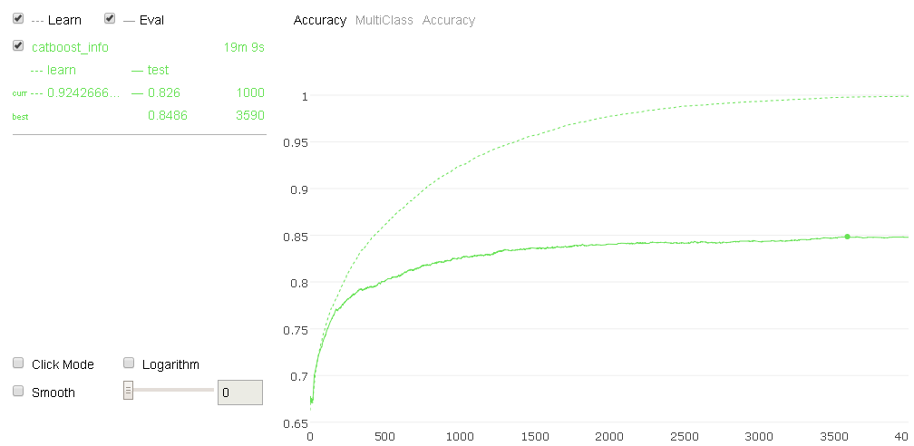
4. We then start training, setting verbosity off but allowing a visual representation of the training and its results, both in-sample and, more importantly, out-of-sample:

In: model.fit(covertype_train, eval_set=covertype_val, 
              verbose=False, plot=True)

Here is an example of what visualization you can get for the model trained on the CoverType dataset:

5. After training, we simply predict the class and its associated probability:

In: preds_class = model.predict(covertype_test) 
    preds_proba = model.predict_proba(covertype_test)

6. An accuracy evaluation points out that the results are equivalent to XGBoost (0.847  against 848) and the confusion matrix looks much cleaner, pointing out a better classification job done by this algorithm:

In: from sklearn.metrics import accuracy_score, confusion_matrix 
    print('test accuracy:', accuracy_score(covertype_test_y, 
                                           preds_class))
    print(confusion_matrix(covertype_test_y, preds_class))

Out: test accuracy:  0.847
     [[1482  320    0    0    0    0   18] 
      [ 213 2199   12    0   10   12    2] 
      [   0   13  260    5    0   23    0] 
      [   0    0    6   18    0    3    0] 
      [   2   40    5    0   30    0    0] 
      [   0   16   33    1    0   94    0] 
      [  31    0    0    0    0    0  152]]