Chapter 4
Reviewing Basic Python
In This Chapter
![]() Using numbers and logic
Using numbers and logic
![]() Interacting with strings
Interacting with strings
![]() Delving into dates
Delving into dates
![]() Developing modular code
Developing modular code
![]() Making decisions and performing tasks repetitively
Making decisions and performing tasks repetitively
![]() Organizing information into sets, lists, and tuples
Organizing information into sets, lists, and tuples
![]() Iterating through data
Iterating through data
![]() Making data easier to find using dictionaries
Making data easier to find using dictionaries
Chapter 3 helped you create a Python installation that’s specific to data science. However, you can use this installation to perform common Python tasks as well, and that’s actually the best way to test your setup to know that it works as intended. If you already know Python, you might be able to skip this chapter and move on to the next chapter; however, it’s probably best to skim the material as a minimum and test some of the examples, just to be sure you have a good installation.
The focus of this chapter is to provide you with a good overview of how Python works as a language. Of course, part of that focus is how you use Python to solve data science problems. However, you can’t use this book to learn Python from scratch. To learn Python from scratch, you need a book such as my book Beginning Programming with Python For Dummies (published by John Wiley & Sons, Inc.) or a tutorial such as the one at https://docs.python.org/2/tutorial/. The chapter assumes that you’ve worked with other programming languages and have at least an idea of how Python works. This limitation aside, the chapter gives you a good reminder of how things work in Python, which is all that many people really need.
 This book uses Python 2.7.x. The latest version of Python as of this writing is version 2.7.9. If you try to use this book with Python 3.4.2 (or above), you may need to modify the examples to compensate for the differences in that version. The “Using Python 2.7.x for this book” sidebar in Chapter 3 provides you with details about Python version differences. Going through the examples in this chapter will help you know what to expect with other examples in the book should you decide to use version 3.4.2 when solving data science problems.
Working with Numbers and Logic
Data science involves working with data of various sorts, but much of the work involves numbers. In addition, you use logical values to make decisions about the data you use. For example, you might need to know whether two values are equal or whether one value is greater than another value. Python supports these number and logic value types:
- Any whole number is an integer. For example, the value 1 is a whole number, so it’s an integer. On the other hand, 1.0 isn’t a whole number; it has a decimal part to it, so it’s not an integer. Integers are represented by the
intdata type. On most platforms, you can store numbers between –9,223,372,036,854,775,808 and 9,223,372,036,854,775,807 within anint(which is the maximum value that fits in a 64-bit variable). - Any number that includes a decimal portion is a floating point value. For example, 1.0 has a decimal part, so it’s a floating-point value. Many people get confused about whole numbers and floating-point numbers, but the difference is easy to remember. If you see a decimal in the number, it’s a floating-point value. Python stores floating-point values in the
floatdata type. The maximum value that a floating-point variable can contain is ±1.7976931348623157 × 10308 and the minimum value that a floating point variable can contain is ±2.2250738585072014 × 10-308 on most platforms. - A complex number consists of a real number and an imaginary number that are paired together. Just in case you’ve completely forgotten about complex numbers, you can read about them at
http://www.mathsisfun.com/numbers/complex-numbers.html. The imaginary part of a complex number always appears with a j after it. So, if you want to create a complex number with 3 as the real part and 4 as the imaginary part, you make an assignment like this:myComplex = 3 + 4j. - Logical arguments require Boolean values, which are named after George Bool. When using a Boolean value in Python, you rely on the
booltype. A variable of this type can contain only two values:TrueorFalse. You can assign a value by using theTrueorFalsekeywords, or you can create an expression that defines a logical idea that equates to true or false. For example, you could saymyBool = 1 > 2, which would equate to False because 1 is most definitely not greater than 2.
Now that you have the basics down, it’s time to see the data types in action. The following paragraphs provide a quick overview of how you can work with both numeric and logical data in Python.
Performing variable assignments
When working with applications, you store information in variables. A variable is a kind of storage box. Whenever you want to work with the information, you access it using the variable. If you have new information you want to store, you put it in a variable. Changing information means accessing the variable first and then storing the new value in the variable. Just as you store things in boxes in the real world, so you store things in variables (a kind of storage box) when working with applications. To store data in a variable, you assign the data to it using any of a number of assignment operators (special symbols that tell how to store the data). Table 4-1 shows the assignment operators that Python supports.
Table 4-1 Python Assignment Operators
Operator |
Description |
Example |
= |
Assigns the value found in the right operand to the left operand |
MyVar = 2 results in MyVar containing 2 |
+= |
Adds the value found in the right operand to the value found in the left operand and places the result in the left operand |
MyVar += 2 results in MyVar containing 7 |
-= |
Subtracts the value found in the right operand from the value found in the left operand and places the result in the left operand |
MyVar -= 2 results in MyVar containing 3 |
*= |
Multiplies the value found in the right operand by the value found in the left operand and places the result in the left operand |
MyVar *= 2 results in MyVar containing 10 |
/= |
Divides the value found in the left operand by the value found in the right operand and places the result in the left operand |
MyVar /= 2 results in MyVar containing 2.5 |
%= |
Divides the value found in the left operand by the value found in the right operand and places the remainder in the left operand |
MyVar %= 2 results in MyVar containing 1 |
**= |
Determines the exponential value found in the left operand when raised to the power of the value found in the right operand and places the result in the left operand |
MyVar ** 2 results in MyVar containing 25 |
//= |
Divides the value found in the left operand by the value found in the right operand and places the integer (whole number) result in the left operand |
MyVar //= 2 results in MyVar containing 2 |
Doing arithmetic
Storing information in variables makes it easily accessible. However, in order to perform any useful work with the variable, you usually perform some type of arithmetic operation on it. Python supports the common arithmetic operators you use to perform tasks by hand. They appear in Table 4-2.
Table 4-2 Python Arithmetic Operators
Operator |
Description |
Example |
+ |
Adds two values together |
5 + 2 = 7 |
- |
Subtracts the right-hand operand from left operand |
5 – 2 = 3 |
* |
Multiplies the right-hand operand by the left operand |
5 * 2 = 10 |
/ |
Divides the left-hand operand by the right operand |
5 / 2 = 2.5 |
% |
Divides the left-hand operand by the right operand and returns the remainder |
5 % 2 = 1 |
** |
Calculates the exponential value of the right operand by the left operand |
5 ** 2 = 25 |
// |
Performs integer division, in which the left operand is divided by the right operand and only the whole number is returned (also called floor division) |
5 // 2 = 2 |
Sometimes you need to interact with just one variable. Python supports a number of unary operators, those that work with just one variable, as shown in Table 4-3.
Table 4-3 Python Unary Operators
Operator |
Description |
Example |
~ |
Inverts the bits in a number so that all of the 0 bits become 1 bits and vice versa. |
~4 results in a value of –5 |
- |
Negates the original value so that positive becomes negative and vice versa. |
–(–4) results in 4 and –4 results in –4 |
+ |
Is provided purely for the sake of completeness. This operator returns the same value that you provide as input. |
+4 results in a value of 4 |
Computers can perform other sorts of math tasks because of the way in which the processor works. It’s important to remember that computers store data as a series of individual bits. Python makes it possible to access these individual bits using bitwise operators, as shown in Table 4-4.
Table 4-4 Python Bitwise Operators
Operator |
Description |
Example |
& (And) |
Determines whether both individual bits within two operators are true and sets the resulting bit to true when they are. |
0b1100 & 0b0110 = 0b0100 |
| (Or) |
Determines whether either of the individual bits within two operators are true and sets the resulting bit to true when they are. |
0b1100 | 0b0110 = 0b1110 |
^ (Exclusive or) |
Determines whether just one of the individual bits within two operators is true and sets the resulting bit to true when one is. When both bits are true or both bits are false, the result is false. |
0b1100 ^ 0b0110 = 0b1010 |
~ (One’s complement) |
Calculates the one’s complement value of a number. |
~0b1100 = –0b1101 ~0b0110 = –0b0111 |
<< (Left shift) |
Shifts the bits in the left operand left by the value of the right operand. All new bits are set to 0 and all bits that flow off the end are lost. |
0b00110011 << 2 = 0b11001100 |
>> (Right shift) |
Shifts the bits in the left operand right by the value of the right operand. All new bits are set to 0 and all bits that flow off the end are lost. |
0b00110011 >> 2 = 0b00001100 |
Comparing data using Boolean expressions
Using arithmetic to modify the content of variables is a kind of data manipulation. To determine the effect of data manipulation, a computer must compare the current state of the variable against its original state or the state of a known value. In some cases, detecting the status of one input against another is also necessary. All these operations check the relationship between two variables, so the resulting operators are relational operators, as shown in Table 4-5.
Table 4-5 Python Relational Operators
Operator |
Description |
Example |
== |
Determines whether two values are equal. Notice that the relational operator uses two equals signs. A mistake many developers make is using just one equals sign, which results in one value being assigned to another. |
1 == 2 is False |
!= |
Determines whether two values are not equal. Some older versions of Python allowed you to use the <> operator in place of the != operator. Using the <> operator results in an error in current versions of Python. |
1 != 2 is True |
> |
Verifies that the left operand value is greater than the right operand value. |
1 > 2 is False |
< |
Verifies that the left operand value is less than the right operand value. |
1 < 2 is True |
>= |
Verifies that the left operand value is greater than or equal to the right operand value. |
1 >= 2 is False |
<= |
Verifies that the left operand value is less than or equal to the right operand value. |
1 <= 2 is True |
Sometimes a relational operator can’t tell the whole story of the comparison of two values. For example, you might need to check a condition in which two separate comparisons are needed, such as MyAge > 40 and MyHeight < 74. The need to add conditions to the comparison requires a logical operator of the sort shown in Table 4-6.
Table 4-6 Python Logical Operators
Operator |
Description |
Example |
and |
Determines whether both operands are true. |
True and True is True True and False is False False and True is False False and False is False |
or |
Determines when one of two operands is true. |
True or True is True True or False is True False or True is True False or False is False |
not |
Negates the truth value of a single operand. A true value becomes false and a false value becomes true. |
not True is False not False is True |
Computers provide order to comparisons by making some operators more significant than others. The ordering of operators is operator precedence. Table 4-7 shows the operator precedence of all the common Python operators, including a few you haven’t seen as part of a discussion yet. When making comparisons, always consider operator precedence because otherwise, the assumptions you make about a comparison outcome will likely be wrong.
Table 4-7 Python Operator Precedence
Operator |
Description |
() |
You use parentheses to group expressions and to override the default precedence so that you can force an operation of lower precedence (such as addition) to take precedence over an operation of higher precedence (such as multiplication). |
** |
Exponentiation raises the value of the left operand to the power of the right operand. |
~ + - |
Unary operators interact with a single variable or expression. |
* / % // |
Multiply, divide, modulo, and floor division. |
+ - |
Addition and subtraction. |
>> << |
Right and left bitwise shift. |
& |
Bitwise AND. |
^ | |
Bitwise exclusive OR and standard OR. |
<= < > >= |
Comparison operators. |
== != |
Equality operators. |
= %= /= //= -= += *= **= |
Assignment operators. |
is is not |
Identity operators. |
in not in |
Membership operators. |
not or and |
Logical operators. |
Creating and Using Strings
Of all the data types, strings are the most easily understood by humans and not understood at all by computers. A string is simply any grouping of characters you place within double quotation marks. For example, myString = "Python is a great language." assigns a string of characters to myString.
The computer doesn’t see letters at all. Every letter you use is represented by a number in memory. For example, the letter A is actually the number 65. To see this for yourself, type ord("A") at the Python prompt and press Enter. You see 65 as output. It’s possible to convert any single letter to its numeric equivalent using the ord() command.
Because the computer doesn’t really understand strings, but strings are so useful in writing applications, you sometimes need to convert a string to a number. You can use the int() and float() commands to perform this conversion. For example, if you type myInt = int("123") and press Enter at the Python prompt, you create an int named myInt that contains the value 123.
You can convert numbers to a string as well by using the str() command. For example, if you type myStr = str(1234.56) and press Enter, you create a string containing the value "1234.56" and assign it to myStr. The point is that you can go back and forth between strings and numbers with great ease. Later chapters demonstrate how these conversions make many seemingly impossible tasks quite doable.
As with numbers, you can use some special operators with strings (and many objects). The member operators make it possible to determine when a string contains specific content. Table 4-8 shows these operators.
Table 4-8 Python Membership Operators
Operator |
Description |
Example |
in |
Determines whether the value in the left operand appears in the sequence found in the right operand |
“Hello” in “Hello Goodbye“ is True |
not in |
Determines whether the value in the left operand is missing from the sequence found in the right operand |
“Hello“ not in “Hello Goodbye“ is False |
The discussion in this section also makes it obvious that you need to know the kind of data that variables contain. You use the identity operators to perform this task, as shown in Table 4-9.
Table 4-9 Python Identity Operators
Operator |
Description |
Example |
is |
Evaluates to true when the type of the value or expression in the right operand points to the same type in the left operand |
type(2) is int is True |
is not |
Evaluates to true when the type of the value or expression in the right operand points to a different type than the value or expression in the left operand |
type(2) is not int is False |
Interacting with Dates
Dates and times are items that most people work with quite a bit. Society bases almost everything on the date and time that a task needs to be or was completed. We make appointments and plan events for specific dates and times. Most of our day revolves around the clock. Because of the time-oriented nature of humans, it’s a good idea to look at how Python deals with interacting with date and time (especially storing these values for later use). As with everything else, computers understand only numbers — date and time don’t really exist.
To work with dates and times, you must issue a special import datetime command. Technically, this act is called importing a module. Don’t worry how the command works right now — just use it whenever you want to do something with date and time.
Computers do have clocks inside them, but the clocks are for the humans using the computer. Yes, some software also depends on the clock, but again, the emphasis is on human needs rather than anything the computer might require. To get the current time, you can simply type datetime.datetime.now() and press Enter. You see the full date and time information as found on your computer’s clock (see Figure 4-1).

Figure 4-1: Get the current date and time using the now() command.
You may have noticed that the date and time are a little hard to read in the existing format. Say that you want to get just the current date, and in a readable format. To accomplish this task, you access just the date portion of the output and convert it into a string. Type str(datetime.datetime.now().date()) and press Enter. Figure 4-2 shows that you now have something a little more usable.

Figure 4-2: Make the date and time more readable using the str() command.
Interestingly enough, Python also has a time() command, which you can use to obtain the current time. You can obtain separate values for each of the components that make up date and time using the day, month, year, hour, minute, second, and microsecond values. Later chapters help you understand how to use these various date and time features to make working with data science applications easier.
Creating and Using Functions
To manage information properly, you need to organize the tools used to perform the required tasks. Each line of code that you create performs a specific task, and you combine these lines of code to achieve a desired result. Sometimes you need to repeat the instructions with different data, and in some cases your code becomes so long that it’s hard to keep track of what each part does. Functions serve as organization tools that keep your code neat and tidy. In addition, functions make it easy to reuse the instructions you’ve created as needed with different data. This section of the chapter tells you all about functions. More important, in this section you start creating your first serious applications in the same way that professional developers do.
Creating reusable functions
You go to your closet, take out pants and shirt, remove the labels, and put them on. At the end of the day, you take everything off and throw it in the trash. Hmmm … that really isn’t what most people do. Most people take the clothes off, wash them, and then put them back into the closet for reuse. Functions are reusable, too. No one wants to keep repeating the same task; it becomes monotonous and boring. When you create a function, you define a package of code that you can use over and over to perform the same task. All you need to do is tell the computer to perform a specific task by telling it which function to use. The computer faithfully executes each instruction in the function absolutely every time you ask it to do so.
When you work with functions, the code that needs services from the function is named the caller, and it calls upon the function to perform tasks for it. Much of the information you see about functions refers to the caller. The caller must supply information to the function, and the function returns information to the caller.
At one time, computer programs didn’t include the concept of code reusability. As a result, developers had to keep reinventing the same code. It didn’t take long for someone to come up with the idea of functions, though, and the concept has evolved over the years until functions have become quite flexible. You can make functions do anything you want. Code reusability is a necessary part of applications to
- Reduce development time
- Reduce programmer error
- Increase application reliability
- Allow entire groups to benefit from the work of one programmer
- Make code easier to understand
- Improve application efficiency
In fact, functions do a whole list of things for applications in the form of reusability. As you work through the examples in this book, you see how reusability makes your life significantly easier. If not for reusability, you’d still be programming by plugging 0s and 1s into the computer by hand.
Creating a function doesn’t require much work. To see how functions work, open a copy of IPython and type in the following code (pressing Enter at the end of each line):
def SayHello():
print('Hello There!')
To end the function, you press Enter a second time after the last line. A function begins with the keyword def (for define). You provide a function name, parentheses that can contain function arguments (data used in the function), and a colon. The editor automatically indents the next line for you. Python relies on whitespace to define code blocks (statements that are associated with each other in a function).
You can now use the function. Simply type SayHello( ) and press Enter. The parentheses after the function name are important because they tell Python to execute the function, rather than tell you that you are accessing a function as an object (to determine what it is). Figure 4-3 shows the output from this function.
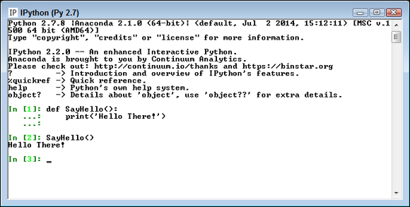
Figure 4-3: Creating and using functions is straightforward.
Calling functions in a variety of ways
Functions can accept arguments (additional bits of data) and return values. The ability to exchange data makes functions far more useful than they otherwise might be. The following sections describe how to call functions in a variety of ways to both send and receive data.
Sending required arguments
A function can require the caller to provide arguments to it. A required argument is a variable that must contain data for the function to work. Open a copy of IPython and type the following code:
def DoSum(Value1, Value2):
return Value1 + Value2
You have a new function, DoSum(). This function requires that you provide two arguments to use it. At least, that’s what you’ve heard so far. Type DoSum() and press Enter. You see an error message, as shown in Figure 4-4, telling you that DoSum requires two arguments.

Figure 4-4: You must supply an argument or you get an error message.
Trying DoSum() with just one argument would result in another error message. In order to use DoSum() you must provide two argument. To see how this works, type DoSum(1, 2) and press Enter. You see the result in Figure 4-5.

Figure 4-5: Supplying two arguments provides the expected output.
Notice that DoSum() provides an output value of 3 when you supply 1 and 2 as inputs. The return statement provides the output value. Whenever you see return in a function, you know the function provides an output value.
Sending arguments by keyword
As your functions become more complex and the methods to use them do as well, you may want to provide a little more control over precisely how you call the function and provide arguments to it. Until now, you have positional arguments, which means that you have supplied values in the order in which they appear in the argument list for the function definition. However, Python also has a method for sending arguments by keyword. In this case, you supply the name of the argument followed by an equals sign (=) and the argument value. To see how this works, open a copy of IPython and type the following code:
def DisplaySum(Value1, Value2):
print(str(Value1) + ' + ' + str(Value2) + ' = ' +
str((Value1 + Value2)))
Notice that the print() function argument includes a list of items to print and that those items are separated by plus signs (+). In addition, the arguments are of different types, so you must convert them using the str() function. Python makes it easy to mix and match arguments in this manner. This function also introduces the concept of automatic line continuation. The print() function actually appears on two lines, and Python automatically continues the function from the first line to the second.
Next, it’s time to test DisplaySum(). Of course, you want to try the function using positional arguments first, so type DisplaySum(2, 3) and press Enter. You see the expected output of 2 + 3 = 5. Now type DisplaySum(Value2 = 3, Value1 = 2) and press Enter. Again, you receive the output 2 + 3 = 5 even though the position of the arguments has been reversed.
Giving function arguments a default value
Whether you make the call using positional arguments or keyword arguments, the functions to this point have required that you supply a value. Sometimes a function can use default values when a common value is available. Default values make the function easier to use and less likely to cause errors when a developer doesn’t provide an input. To create a default value, you simply follow the argument name with an equals sign and the default value. To see how this works, open a copy of IPython and type the following code:
def SayHello(Greeting = "No Value Supplied"):
print(Greeting)
The SayHello() function provides an automatic value for Greeting when a caller doesn’t provide one. When someone tries to call SayHello() without an argument, it doesn’t raise an error. Type SayHello() and press Enter to see for yourself — you see the default message. Type SayHello("Howdy!") to see a normal response.
Creating functions with a variable number of arguments
In most cases, you know precisely how many arguments to provide with your function. It pays to work toward this goal whenever you can because functions with a fixed number of arguments are easier to troubleshoot later. However, sometimes you simply can’t determine how many arguments the function will receive at the outset. For example, when you create a Python application that works at the command line, the user might provide no arguments, the maximum number of arguments (assuming there is one), or any number of arguments in between.
Fortunately, Python provides a technique for sending a variable number of arguments to a function. You simply create an argument that has an asterisk in front of it, such as *VarArgs. The usual technique is to provide a second argument that contains the number of arguments passed as an input. To see how this works, open a copy of IPython and type the following code:
def DisplayMulti(ArgCount = 0, *VarArgs):
print('You passed ' + str(ArgCount) + ' arguments.',
Var Args)
Notice that the print() function displays a string and then the list of arguments. Because of the way this function is designed, you can type DisplayMulti( ) and press Enter to see that it’s possible to pass zero arguments. To see multiple arguments at work, type DisplayMulti(3, 'Hello', 1, True) and press Enter. The output of ('You passed 3 arguments.', ('Hello', 1, True)) shows that you need not pass values of any particular type.
Using Conditional and Loop Statements
Computer applications aren’t very useful if they perform precisely the same tasks the same number of times every time you run them. Yes, they can perform useful work, but life seldom offers situations in which conditions remain the same. In order to accommodate changing conditions, applications must make decisions and perform tasks a variable number of times. Conditional and loop statements make it possible to perform this task as described in the sections that follow.
Making decisions using the if statement
You use “if” statements regularly in everyday life. For example, you may say to yourself, “If it’s Wednesday, I’ll eat tuna salad for lunch.” The Python if statement is a little less verbose, but it follows precisely the same pattern. To see how this works, open a copy of IPython and type the following code:
def TestValue(Value):
if Value == 5:
print('Value equals 5!')
elif Value == 6:
print('Value equals 6!')
else:
print('Value is something else.')
print('It equals ' + str(Value))
Every Python if statement begins, oddly enough, with the word if. When Python sees if, it knows that you want it to make a decision. After the word if comes a condition. A condition simply states what sort of comparison you want Python to make. In this case, you want Python to determine whether Value contains the value 5.
Notice that the condition uses the relational equality operator, ==, and not the assignment operator, =. A common mistake that developers make is to use the assignment operator rather than the equality operator.
The condition always ends with a colon (:). If you don’t provide a colon, Python doesn’t know that the condition has ended and will continue to look for additional conditions on which to base its decision. After the colon comes any tasks you want Python to perform.
You may need to perform multiple tasks using a single if statement. The elif clause makes it possible to add an additional condition and associated tasks. A clause is an addendum to a previous condition, which is an if statement in this case. The elif clause always provides a condition, just like the if statement, and it has its own associated set of tasks to perform.
Sometimes you need to do something no matter what the condition might be. In this case, you add the else clause. The else clause tells Python to do something in particular when the conditions of the if statement aren’t met.
Notice how indenting is becoming more important as the functions become more complex. The function contains an if statement. The if statement contains just one print() statement. The else clause contains two print() statements.
To see this function in action, type TestValue(1) and press Enter. You see the output from the else clause. Type TestValue(5) and press Enter. The output now reflects the if statement output. Type TestValue(6) and press Enter. The output now shows the results of the elif clause. The result is that this function is more flexible than previous functions in the chapter because it can make decisions.
Choosing between multiple options using nested decisions
Nesting is the process of placing a subordinate statement within another statement. You can nest any statement within any other statement in most cases. To see how this works, open a copy of IPython and type the following code:
def SecretNumber():
One = int(input("Type a number between 1 and 10: "))
Two = int(input("Type a number between 1 and 10: "))
if (One >= 1) and (One <= 10):
if (Two >= 1) and (Two <= 10):
print('Your secret number is: ' + str(One * Two))
else:
print("Incorrect second value!")
else:
print("Incorrect first value!")
In this case, SecretNumber() asks you to provide two inputs. Yes, you can get inputs from a user when needed by using the input() function. The int() function converts the inputs to a number.
There are two levels of if statement this time. The first level checks for the validity of the number in One. The second level checks for the validity of the number in Two. When both One and Two have values between 1 and 10, then SecretNumber() outputs a secret number for the user.
To see SecretNumber() in action, type SecretNumber() and press Enter. Type 20 and press Enter when asked for the first input value, and type 10 and press Enter when asked for the second. You see an error message telling you that the first value is incorrect. Type SecretNumber() and press Enter again. This time, use values of 10 and 20. The function will tell you that the second input is incorrect. Try the same sequence again using input values of 10 and 10.
Performing repetitive tasks using for
Sometimes you need to perform a task more than one time. You use the for loop statement when you need to perform a task a specific number of times. The for loop has a definite beginning and a definite end. The number of times that that loop executes depends on the number of elements in the variable you provide. To see how this works, open a copy of IPython and type the following code:
def DisplayMulti(*VarArgs):
for Arg in VarArgs:
if Arg.upper() == 'CONT':
continue
print('Continue Argument: ' + Arg)
elif Arg.upper() == 'BREAK':
break
print('Break Argument: ' + Arg)
print('Good Argument: ' + Arg)
In this case, the for loop attempts to process each element in VarArgs. Notice that there is a nested if statement in the loop and it tests for two ending conditions. In most cases, the code skips the if statement and simply prints the argument. However, when the if statement finds the words CONT or BREAK in the input values, it performs one of these two tasks:
continue: Forces the loop to continue from the current point of execution with the next entry in VarArgs.break: Stops the loop from executing.
 The keywords can appear capitalized in any way because the
 upper() function converts them to uppercase. The DisplayMulti() function can process any number of input strings. To see it in action, type DisplayMulti('Hello', 'Goodbye', 'First', 'Last') and press Enter. You see each of the input strings presented on a separate line in the output. Now type DisplayMulti('Hello', 'Cont', 'Goodbye', 'Break', 'Last') and press Enter. Notice that the words Cont and Break don’t appear in the output because they’re keywords. In addition, the word Last doesn’t appear in the output because the for loop ends before this word is processed.
Using the while statement
The while loop statement continues to perform tasks until such time that a condition is no longer true. As with the for statement, the while statement supports both the continue and break keywords for ending the loop prematurely. To see how this works, open a copy of IPython and type the following code:
def SecretNumber():
GotIt = False
while GotIt == False:
One = int(input("Type a number between 1 and 10: "))
Two = int(input("Type a number between 1 and 10: "))
if (One >= 1) and (One <= 10):
if (Two >= 1) and (Two <= 10):
print('Secret number is: ' + str(One * Two))
GotIt = True
continue
else:
print("Incorrect second value!")
else:
print("Incorrect first value!")
print("Try again!")
This is an expansion of the SecretNumber() function first described in the “Choosing between multiple options using nested decisions” section, earlier in this chapter. However, in this case, the addition of a while loop statement means that the function continues to ask for input until it receives a valid response.
To see how the while statement works, type SecretNumber( ) and press Enter. Type 20 and press Enter for the first prompt. Type 10 and press Enter for the second prompt. The example tells you that the first number is wrong and then tells you to try again. Try a second time using values of 10 and 20. This time the second number is wrong and you still need to try again. On the third try, use values of 10 and 10. This time you get a secret number. Notice that the use of a continue clause means that the application doesn’t tell you to try again.
Storing Data Using Sets, Lists, and Tuples
Python provides a host of methods for storing data in memory. Each method has advantages and disadvantages. Choosing the most appropriate method for your particular need is important. The following sections discuss three common techniques used for storing data for data science needs.
Performing operations on sets
Most people have used sets at one time or another in school to create lists of items that belong together. These lists then became the topic of manipulation using math operations such as intersection, union, difference, and symmetric difference. Sets are the best option to choose when you need to perform membership testing and remove duplicates from a list. You can’t perform sequence-related tasks using sets, such a indexing or slicing. To see how you can work with sets, start a copy of IPython and type the following code:
from sets import Set
SetA = Set(['Red', 'Blue', 'Green', 'Black'])
SetB = Set(['Black', 'Green', 'Yellow', 'Orange'])
SetX = SetA.union(SetB)
SetY = SetA.intersection(SetB)
SetZ = SetA.difference(SetB)
Notice that you must import the Set capability into your Python application. The module sets contain a Set class that you import into your application in order to use the resulting functionality. If you try to use the Set class without first importing it, Python displays an error message. The book uses a number of imported libraries, so knowing how to use the import statement is important.
You now have five different sets to play with, each of which has some common elements. To see the results of each math operation, type print '{0} {1} {2}'.format(SetX, SetY, SetZ) and press Enter. You see one set printed on each line, like this:
Set(['Blue', 'Yellow', 'Green', 'Orange', 'Black', 'Red'])
Set(['Green', 'Black'])
Set(['Blue', 'Red'])
The outputs show the results of the math operations: union(), intersection(), and difference(). (When working with Python 3.4, the output may vary from the Python 2.7 output shown. All output in the book is for Python 2.7, so you may see differences from time to time when using Python 3.4.) Python’s fancier print formatting can be useful in working with collections such as sets. The format() function tells Python which objects to place within each of the placeholders in the string. A placeholder is a set of curly brackets ({}) with an optional number in it. The escape character (essentially a kind of control or special character), /n, provides a newline character between entries. You can read more about fancy formatting at https://docs.python.org/2/tutorial/inputoutput.html.
You can also test relationships between the various sets. For example, type SetA.issuperset(SetY) and press Enter. The output value of True tells you that SetA is a superset of SetY. Likewise, if you type SetA.issubset(SetX) and press Enter, you find that SetA is a subset of SetX.
It’s important to understand that sets are either mutable or immutable. All the sets in this example are mutable, which means that you can add or remove elements from them. For example, if you type SetA.add('Purple') and press Enter, SetA receives a new element. If you type SetA.issubset(SetX) and press Enter now, you find that SetA is no longer a subset of SetX because SetA has the 'Purple' element in it.
Working with lists
The Python specification defines a list as a kind of sequence. Sequences simply provide some means of allowing multiple data items to exist together in a single storage unit, but as separate entities. Think about one of those large mail holders you see in apartment buildings. A single mail holder contains a number of small mailboxes, each of which can contain mail. Python supports other kinds of sequences as well:
- Tuples: A tuple is a collection used to create complex list-like sequences. An advantage of tuples is that you can nest the content of a tuple. This feature lets you create structures that can hold employee records or x-y coordinate pairs.
- Dictionaries: As with the real dictionaries, you create key/value pairs when using the dictionary collection (think of a word and its associated definition). A dictionary provides incredibly fast search times and makes ordering data significantly easier.
- Stacks: Most programming languages support stacks directly. However, Python doesn’t support the stack, although there’s a workaround for that. A stack is a first in/first out (LIFO) sequence. Think of a pile of pancakes: You can add new pancakes to the top and also take them off of the top. A stack is an important collection that you can simulate in Python using a list.
- Queues: A queue is a last in/first out (FIFO) collection. You use it to track items that need to be processed in some way. Think of a queue as a line at the bank. You go into the line, wait your turn, and are eventually called to talk with a teller.
- Deques: A double-ended queue (deque) is a queue-like structure that lets you add or remove items from either end, but not from the middle. You can use a deque as a queue or a stack or any other kind of collection to which you’re adding and from which you’re removing items in an orderly manner (in contrast to lists, tuples, and dictionaries, which allow randomized access and management).
Of all the sequences, lists are the easiest to understand and are the most directly related to a real-world object. Working with lists helps you become better able to work with other kinds of sequences that provide greater functionality and improved flexibility. The point is that the data is stored in a list much as you would write it on a piece of paper — one item comes after another. The list has a beginning, a middle, and an end. As shown in the figure, the items are numbered. (Even if you might not normally number them in real life, Python always numbers the items for you.) To see how you can work with lists, start a copy of IPython and type the following code:
ListA = [0, 1, 2, 3]
ListB = [4, 5, 6, 7]
ListA.extend(ListB)
ListA
When you type the last line of code, you see the output of [0, 1, 2, 3, 4, 5, 6, 7]. The extend() function adds the members of ListB to ListA. Beside extending lists, you can also add to them using the append() function. Type ListA.append(-5) and press Enter. When you type ListA and press Enter again, you see that Python has added –5 to the end of the list. You may find that you need to remove items again and you do that using the remove() function. For example, type ListA.remove(-5) and press Enter. When you list ListA again, you see that the added entry is gone.
Lists also support concatenation using the plus (+) sign. For example, if you type ListX = ListA + ListB and press Enter, you find that the newly created ListX contains both ListA and ListB in it with the elements of ListA coming first.
Creating and using Tuples
A tuple is a collection used to create complex lists, in which you can embed one tuple within another. This embedding lets you create hierarchies with tuples. A hierarchy could be something as simple as the directory listing of your hard drive or an organizational chart for your company. The idea is that you can create complex data structures using a tuple.
Tuples are immutable, which means you can’t change them. You can create a new tuple with the same name and modify it in some way, but you can’t modify an existing tuple. Lists are mutable, which means that you can change them. So, a tuple can seem at first to be at a disadvantage, but immutability has all sorts of advantages, such as being more secure as well as faster. In addition, immutable objects are easier to use with multiple processors. To see how you can work with tuples, start a copy of IPython and type the following code:
MyTuple = (1, 2, 3, (4, 5, 6, (7, 8, 9)))
MyTuple is nested three levels deep. The first level consists of the values 1, 2, and 3, and a tuple. The second level consists of the values 4, 5, and 6, and yet another tuple. The third level consists of the values 7, 8, and 9. To see how this works, type the following code into IPython:
for Value1 in MyTuple:
if type(Value1) == int:
print Value1
else:
for Value2 in Value1:
if type(Value2) == int:
print " ", Value2
else:
for Value3 in Value2:
print " ", Value3
When you run this code, you find that the values really are at three different levels. You can see the indentations showing the level:
1
2
3
4
5
6
7
8
9
It is possible to perform tasks such as adding new values, but you must do it by adding the original entries and the new values to a new tuple. In addition, you can add tuples to an existing tuple only. To see how this works, type MyNewTuple = MyTuple.__add__((10, 11, 12, (13, 14, 15))) and press Enter. MyNewTuple contains new entries at both the first and second levels, like this: (1, 2, 3, (4, 5, 6, (7, 8, 9)), 10, 11, 12, (13, 14, 15)). If you were to run the previous code against MyNewTuple, you’d see entries at the appropriate levels in the output, as shown here.
1
2
3
4
5
6
7
8
9
10
11
12
13
14
15
Defining Useful Iterators
The chapters that follow use all kinds of techniques to access individual values in various types of data structures. For this section, you use two simple lists, defined as the following:
ListA = ['Orange', 'Yellow', 'Green', 'Brown']
ListB = [1, 2, 3, 4]
The simplest method of accessing a particular value is to use an index. For example, if you type ListA[1] and press Enter, you see 'Yellow' as the output. All indexes in Python are zero-based, which means that the first entry is 0, not 1.
Ranges present another simple method of accessing values. For example, if you type ListB[1:3] and press Enter, the output is [2, 3]. You could use the range as input to a for loop, such as
for Value in ListB[1:3]:
print Value
Instead of the entire list, you see just 2 and 3 as outputs, printed on separate lines. The range has two values separated by a colon. However, the values are optional. For example, ListB[:3] would output [1, 2, 3]. When you leave out a value, the range starts at the beginning or the end of the list, as appropriate.
Sometimes you need to process two lists in parallel. The simplest method of doing this is to use the zip() function. Here’s an example of the zip() function in action:
for Value1, Value2 in zip(ListA, ListB):
print Value1, ' ', Value2
This code processes both ListA and ListB at the same time. The processing ends when the for loop reaches the shortest of the two lists. In this case, you see the following:
Orange 1
Yellow 2
Green 3
Brown 4
This is the tip of the iceberg. You see a host of iterator types used throughout the book. The idea is to make it possible to list just the items you want, rather than all of the items in a list or other data structure. Some of the iterators used in upcoming chapters are a little more complicated than what you see here, but this is an important start.
Indexing Data Using Dictionaries
A dictionary is a special kind of sequence that uses a name and value pair. The use of a name makes it easy to access particular values with something other than a numeric index. To create a dictionary, you enclose name and value pairs in curly brackets. Create a test dictionary by typing MyDict = {'Orange':1, 'Blue':2, 'Pink':3} and pressing Enter.
To access a particular value, you use the name as an index. For example, type MyDict['Pink'] and press Enter to see the output value of 3. The use of dictionaries as data structures makes it easy to access incredibly complex data sets using terms that everyone can understand. In many other respects, working with a dictionary is the same as working with any other sequence.
Dictionaries do have some special features. For example, type MyDict.keys( ) and press Enter to see a list of the keys. You can use the values() function to see the list of values in the dictionary.