
![]()
Merging and Reshaping Datasets
This chapter covers how to merge datasets, add rows and columns to existing datasets, reshape datasets, and stack and unstack datasets. You will find that some of the analyses you want to do will require stacked data, others will require unstacked data, and still others can use data of either type.
Recipe 4-1. Merging Datasets by a Common Variable
Problem
We often have datasets with one or more common variables and want to combine those datasets by matching on a common variable. The merge() function locates matching variables and combines datasets based on these variables.
Solution
The following hypothetical data represent the information on 20 students and each student’s scores on five quizzes along with the student’s final grade (the average of the quiz scores). See that the only variable the data frames have in common is the student number in column 1.
> studentInfo
   Student    Sex Age
1        1   male  18
2        2   male  19
3        3   male  17
4        4   male  20
5        5 female  23
6        6 female  18
7        7   male  21
8        8 female  20
9        9 female  23
10      10 female  21
11      11 female  23
12      12   male  18
13      13   male  21
14      14   male  17
15      15   male  19
16      16 female  20
17      17 female  19
18      18 female  22
19      19 female  22
20      20   male  20
> studentQuizzes
   Student    Sex Age Quiz1 Quiz2 Quiz3 Quiz4 Quiz5 FinalGrade
1        1   male  18    83    87    81    80    69       69.7
2        2   male  19    76    89    61    85    75       67.5
3        3   male  17    85    86    65    64    81       66.3
4        4   male  20    92    73    76    88    64       68.8
5        5 female  23    82    75    96    87    78       73.5
6        6 female  18    88    73    76    91    81       71.2
7        7   male  21    89    71    61    70    75       64.5
8        8 female  20    89    70    87    76    88       71.7
9        9 female  23    92    85    95    89    62       74.3
10      10 female  21    86    83    77    64    63       65.7
11      11 female  23    90    71    91    86    87       74.7
12      12   male  18    84    71    67    62    70       62.0
13      13   male  21    83    80    89    60    60       65.5
14      14   male  17    79    77    82    63    74       65.3
15      15   male  19    89    80    64    94    78       70.7
16      16 female  20    76    85    65    92    82       70.0
17      17 female  19    92    76    76    74    91       71.3
18      18 female  22    75    90    78    70    76       68.5
19      19 female  22    87    87    63    73    64       66.0
20      20   male  20    75    74    63    91    87       68.3
To merge the datasets, do the following:
> studentComplete <- merge(studentInfo, studentQuizzes)

> studentComplete
   Student    Sex Age Quiz1 Quiz2 Quiz3 Quiz4 Quiz5 FinalGrade
1        1   male  18    83    87    81    80    69       69.7
2       10 female  21    86    83    77    64    63       65.7
3       11 female  23    90    71    91    86    87       74.7
4       12   male  18    84    71    67    62    70       62.0
5       13   male  21    83    80    89    60    60       65.5
6       14   male  17    79    77    82    63    74       65.3
7       15   male  19    89    80    64    94    78       70.7
8       16 female  20    76    85    65    92    82       70.0
9       17 female  19    92    76    76    74    91       71.3
10      18 female  22    75    90    78    70    76       68.5
11      19 female  22    87    87    63    73    64       66.0
12       2   male  19    76    89    61    85    75       67.5
13      20   male  20    75    74    63    91    87       68.3
14       3   male  17    85    86    65    64    81       66.3
15       4   male  20    92    73    76    88    64       68.8
16       5 female  23    82    75    96    87    78       73.5
17       6 female  18    88    73    76    91    81       71.2
18       7   male  21    89    71    61    70    75       64.5
19       8 female  20    89    70    87    76    88       71.7
20       9 female  23    92    85    95    89    62       74.3
Notice that the student numbers are no longer in the original order. R merges on the student number and then sorts on the common variable. But in this case, the number 1 is followed by 10–19, then 2, 20, and 3–9. We can get the numbers back into order by using the order() function, as follows. Note that the row numbers are still the ones associated with the original records, but the new data frame shows the student numbers in order once again.
> studentComplete <- studentComplete[order(studentComplete[1]),]
> head(studentComplete)
   Student    Sex Age Quiz1 Quiz2 Quiz3 Quiz4 Quiz5 FinalGrade
1        1   male  18    83    87    81    80    69       69.7
12       2   male  19    76    89    61    85    75       67.5
14       3   male  17    85    86    65    64    81       66.3
15       4   male  20    92    73    76    88    64       68.8
16       5 female  23    82    75    96    87    78       73.5
17       6 female  18    88    73    76    91    81       71.2
It is possible that the variables on which you would like to merge datasets have different names in the different datasets (remember R is case sensitive). To deal with that situation, you can either rename the variables so that the names match, or you can use the by.x and by.y options in the merge() command. As an example, what if the student numbers had different variable names, such as id in one file and studentID in another, as follows:
> head(studentInfo)
  studentID    Sex Age
1         1   male  18
2         2   male  19
3         3   male  17
4         4   male  20
5         5 female  23
6         6 female  18
> head(studentQuizzes)
  id    Sex Age Quiz1 Quiz2 Quiz3 Quiz4 Quiz5 FinalGrade
1  1   male  18    83    87    81    80    69       69.7
2  2   male  19    76    89    61    85    75       67.5
3  3   male  17    85    86    65    64    81       66.3
4  4   male  20    92    73    76    88    64       68.8
5  5 female  23    82    75    96    87    78       73.5
6  6 female  18    88    73    76    91    81       71.2
The label for the merged column is from the first data frame. See that the sex and age variables were inherited from both data frames and are now labeled by their sources.
> newData <- merge(x=studentInfo, y=studentQuizzes, by.x="studentID", by.y ="id")
> head(newData)
  studentID  Sex.x Age.x  Sex.y Age.y Quiz1 Quiz2 Quiz3 Quiz4 Quiz5 FinalGrade
1         1   male    18   male    18    83    87    81    80    69       69.7
2         2   male    19   male    19    76    89    61    85    75       67.5
3         3   male    17   male    17    85    86    65    64    81       66.3
4         4   male    20   male    20    92    73    76    88    64       68.8
5         5 female    23 female    23    82    75    96    87    78       73.5
6         6 female    18 female    18    88    73    76    91    81       71.2
To eliminate the duplicated columns, you can set them to NULL, as we have discussed previously, or you can tell R to merge on multiple columns to avoid this problem in the first place. I edited both data frames to use the same names for id, sex, and age. Now I simply merge the two data frames as follows:
> merge(studentInfo, studentQuizzes, c("id", "sex", "age"))
   id    sex age Quiz1 Quiz2 Quiz3 Quiz4 Quiz5 FinalGrade
1   1   male  18    83    87    81    80    69       69.7
2  10 female  21    86    83    77    64    63       65.7
3  11 female  23    90    71    91    86    87       74.7
4  12   male  18    84    71    67    62    70       62.0
5  13   male  21    83    80    89    60    60       65.5
6  14   male  17    79    77    82    63    74       65.3
7  15   male  19    89    80    64    94    78       70.7
8  16 female  20    76    85    65    92    82       70.0
9  17 female  19    92    76    76    74    91       71.3
10 18 female  22    75    90    78    70    76       68.5
11 19 female  22    87    87    63    73    64       66.0
12  2   male  19    76    89    61    85    75       67.5
13 20   male  20    75    74    63    91    87       68.3
14  3   male  17    85    86    65    64    81       66.3
15  4   male  20    92    73    76    88    64       68.8
16  5 female  23    82    75    96    87    78       73.5
17  6 female  18    88    73    76    91    81       71.2
18  7   male  21    89    71    61    70    75       64.5
19  8 female  20    89    70    87    76    88       71.7
20  9 female  23    92    85    95    89    62       74.3
When you merge data frames, R will exclude any observations that appear in only one dataset. Here are some data from the CIA World Factbook web site. We have the economic and demographic data in a CSV file called demographic.csv, and the number of airports in each country in a separate CSV file called airports.csv. After reading those files in with the read.csv() function, I see that they contain data for different countries. The merge will exclude countries not in both datasets. The demographic information covers 46 countries, 45 of which are also in the airport dataset. The airport information includes 236 countries. The merge includes only the countries in both datasets. The final list of countries included in the merged dataset is shown at the end of the following R code:
> head(demographic)
    country      area g20 petroleum population pct65plus lifeExpectancy
1   Algeria 2,381,740   0         2     31,736      4.07          69.95
2 Argentina 2,766,890   1         1     37,385     10.42          75.26
3 Australia 7,686,850   1         1     19,357     12.50          79.87
4   Austria    83,858   0         0      8,150     15.38          77.84
5   Belgium    30,510   0         0     10,259     16.95          77.96
6    Brazil 8,511,965   1         1    174,469      5.45          63.24
  Literacy  GDP labor unempl exports imports cellPhones
1     61.6  5.5   9.1     30    19.6     9.2      0.034
2     96.2 12.9    15     15    26.5    25.2      3.000
3    100.0 23.2   9.5    6.4    69.0    77.0      6.400
4     98.0 25.0   3.7    5.4    63.2    65.6      4.500
5     98.0 25.3  4.34    8.4   181.4   166.0      1.000
6     83.3  6.5    79    7.1    55.1    55.8      4.400
> head(airports)
        country airports
1 United States   13,513
2        Brazil    4,093
3        Mexico    1,714
4        Canada    1,467
5        Russia    1,218
6     Argentina    1,138
> completeCIA <- merge(demographic, airports)
> head(completeCIA)
    country      area g20 petroleum population pct65plus lifeExpectancy
1   Algeria 2,381,740   0         2     31,736      4.07          69.95
2 Argentina 2,766,890   1         1     37,385     10.42          75.26
3 Australia 7,686,850   1         1     19,357     12.50          79.87
4   Austria    83,858   0         0      8,150     15.38          77.84
5   Belgium    30,510   0         0     10,259     16.95          77.96
6    Brazil 8,511,965   1         1    174,469      5.45          63.24
  Literacy  GDP labor unempl exports imports cellPhones airports
1     61.6  5.5   9.1     30    19.6     9.2      0.034      157
2     96.2 12.9    15     15    26.5    25.2      3.000    1,138
3    100.0 23.2   9.5    6.4    69.0    77.0      6.400      480
4     98.0 25.0   3.7    5.4    63.2    65.6      4.500       52
5     98.0 25.3  4.34    8.4   181.4   166.0      1.000       41
6     83.3  6.5    79    7.1    55.1    55.8      4.400    4,093
> length(completeCIA$airports)
[1] 45
> length(demographic$country)
[1] 46
> length(airports$country)
[1] 236
> completeCIA$country
 [1] Algeria              Argentina            Australia
 [4] Austria              Belgium              Brazil
 [7] Canada               China                Czech Republic
[10] Denmark              Finland              France
[13] Germany              Greece               Hungary
[16] Iceland              India                Indonesia
[19] Iran                 Iraq                 Ireland
[22] Italy                Japan                Kuwait
[25] Libya                Luxembourg           Mexico
[28] Netherlands          New Zealand          Nigeria
[31] Norway               Poland               Portugal
[34] Qatar                Russia               Saudi Arabia
[37] South Africa         Spain                Sweden
[40] Switzerland          Turkey               United Arab Emirates
[43] United Kingdom       United States        Venezuela
46 Levels: Algeria Argentina Australia Austria Belgium Brazil Canada ... Venezuela
Recipe 4-2. Adding Rows and Columns
Problem
A common problem is the need to add new rows or columns to a data frame. In Recipe 4-2, you will learn how to do that.
Solution
To add rows and columns of data, you use the rbind() and cbind() functions, respectively. I have a vector containing the weights of 40 adult males who exercise regularly. I want to create a vector of id numbers and combine that vector with the weights. This is a job for the cbind() function. The vector of weights is transformed to a data frame (using the as.data.frame() function), and then the vector of id numbers is bound to the weights, as shown in the following code:
> weights
 [1] 169.1 144.2 179.3 175.8 152.6 166.8 135.0 201.5 175.2 139.0 156.3 186.6
[13] 191.1 151.3 209.4 237.1 176.7 220.6 166.1 137.4 164.2 162.4 151.8 144.1
[25] 204.6 193.8 172.9 161.9 174.8 169.8 213.3 198.0 173.3 214.5 137.1 119.5
[37] 189.1 164.7 170.1 151.0
> weights <- as.data.frame(weights)
> id <- c(1:40)
> id
 [1]  1  2  3  4  5  6  7  8  9 10 11 12 13 14 15 16 17 18 19 20 21 22 23 24 25
[26] 26 27 28 29 30 31 32 33 34 35 36 37 38 39 40
> weights <- cbind(weights, id)
)
> > head(weights)
  weights id
1   169.1  1
2   144.2  2
3   179.3  3
4   175.8  4
5   152.6  5
6   166.8  6
Now, imagine I obtain the weights of another dozen men who exercise regularly. I used the rnorm() function to create the additional data. The rnorm() function produces a random sample of normally distributed scores. I created a 12-element vector with a mean of 175 pounds (lb.) and a standard deviation of 20. The combination of the two vectors produced a matrix, but it is easy to bind it to the data frame.
> extraWeights <- rnorm(12,175,20)
> extraWeights
 [1] 166.8790 191.1003 187.1548 158.1391 136.4888 162.1276 211.9919 189.0800
 [9] 202.9519 205.6483 197.1733 173.3894
> extraWeights <- round(extraWeights, 2)
> extraWeights
 [1] 166.88 191.10 187.15 158.14 136.49 162.13 211.99 189.08 202.95 205.65
[11] 197.17 173.39
> newids <- c(41:52)
> newData <- cbind(extraWeights, newids)
> newData
      extraWeights newids
 [1,]       166.88     41
 [2,]       191.10     42
 [3,]       187.15     43
 [4,]       158.14     44
 [5,]       136.49     45
 [6,]       162.13     46
 [7,]       211.99     47
 [8,]       189.08     48
 [9,]       202.95     49
[10,]       205.65     50
[11,]       197.17     51
[12,]       173.39     52
Next, I made sure the two datasets had the same variable names for the rbind() function to work properly. I used the Data Editor and changed the variable names in newData, as shown in Figure 4-1.

Figure 4-1. Using the Data Editor to change variable names
Then, I combined the data using rbind() and verified that all 52 observations were in the new dataset.
> weights <- rbind(weights, newData)
> summary(weights)
> length(weights$id)
[1] 52
Recipe 4-3. Reshaping a Dataset
Problem
Many repeated-measures datasets have a column for each measurement. For example, here are some repeated-measures data representing the scores on a 20-item test of algebra at the beginning of a statistics course, at the end of the course, and six months later. The wide version has each score in a separate column for each student. The long version has all 30 scores in a single column, and the time of the test is coded 1, 2, 3 for each measurement. The student numbers are repeated, which means that each student’s data occupy 10 rows in the dataset. It's quite common to want to convert from the wide version to the long version, and vice versa.
> wideData
   Student Before After SixMo
1        1     13    15    17
2        2      8     8     7
3        3     12    15    14
4        4     12    17    16
5        5     19    20    20
6        6     10    15    14
7        7     10    13    15
8        8      8    12    11
9        9     14    15    13
10      10     11    16     9
> head(longData)
  Case Student Time Score
1    1       1    1    13
2    2       2    1     8
3    3       3    1    12
4    4       4    1    12
5    5       5    1    19
6    6       6    1    10
> tail(longData)
   Case Student Time Score
25   25       5    3    20
26   26       6    3    14
27   27       7    3    15
28   28       8    3    11
29   29       9    3    13
30   30      10    3     9
Solution
The reshape() function can convert wide format to long format, and long format to wide format. Let us take the wide data first and convert that dataset to long form. I use separate lines to make the function easier to comprehend:
> longScores <- reshape(wideData,
+ direction = "long",
+ varying = list(c("Before","After","SixMo")),
+ times=c(1,2,3),
+ timevar = "Time", idvar = "Student",
+ v.names = "Score")
The reshape() function requires several arguments:
- direction tells R what the desired shape of the new data frame will be.
- varying corresponds to the variable names in the wide format that will become separate variables in the reshaped data.
- times indicates the values to use for the newly created time variable specified by the timevar argument.
- v.names gives the names of the variables in the long format that correspond to multiple variables in the wide format.
We have reshaped the wide dataset into a long dataset (see Figure 4-2).
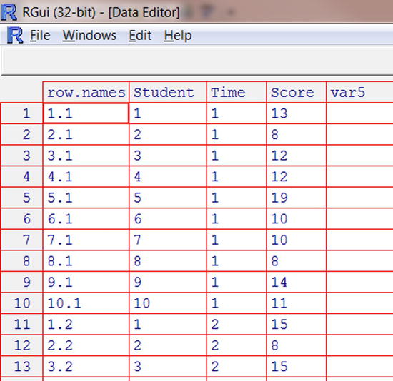
Figure 4-2. The reshaped data in long form
The reshape() function does not require the v.names and timevar arguments. They can be used to give appropriate names to the variables.
Now, let’s reverse the process. We will convert the long dataset back into a wide dataset. The first order of business is to sort the longScores dataset by student number so that each student’s data will occupy three consecutive rows. Changing from one format to the other is often necessary because the data must be in a particular form in order for the analysis to work properly.
> head(longScores)
    Student Time Score
1.1       1    1    13
2.1       2    1     8
3.1       3    1    12
4.1       4    1    12
5.1       5    1    19
6.1       6    1    10

> longScores.sort <- longScores[order(longScores$Student),]
> head(longScores.sort)
    Student Time Score
1.1       1    1    13
1.2       1    2    15
1.3       1    3    17
2.1       2    1     8
2.2       2    2     8
2.3       2    3     7
Now, with the data in the correct format, we can change the long data back into wide data, as follows. Note that the time variable and the id variable are the same as in the previous example:
> wide <- reshape(longScores.sort,timevar = "Time", idvar = "Student", direction = "wide")
> wide
     Student Score.1 Score.2 Score.3
1.1        1      13      15      17
2.1        2       8       8       7
3.1        3      12      15      14
4.1        4      12      17      16
5.1        5      19      20      20
6.1        6      10      15      14
7.1        7      10      13      15
8.1        8       8      12      11
9.1        9      14      15      13
10.1      10      11      16       9
Recipe 4-4. Stacking and Unstacking Data
Problem
Some R functions allow you to use either stacked or unstacked data. For example, here are the scores on a recent 200-point quiz for two sections of my online psychological statistics class. The data are in both stacked and unstacked form. For example, the t.test() function can be used with either stacked or unstacked data, but that is not true of many other analyses, so learning to stack and unstack data as required is a very useful basic R skill.
> unstacked
  section1 section2
1      176      120
2      176      199
3       98      159
4      118      127
5      103      141
6      190      132
7      173      176
8      184       52
9      149      180
> stacked
   score  section
1    176 section1
2    176 section1
3     98 section1
4    118 section1
5    103 section1
6    190 section1
7    173 section1
8    184 section1
9    149 section1
10   120 section2
11   199 section2
12   159 section2
13   127 section2
14   141 section2
15   132 section2
16   176 section2
17    52 section2
18   180 section2
Solution
> stacked <- stack(unstacked)
> stacked
   values      ind
1     176 section1
2     176 section1
3      98 section1
4     118 section1
5     103 section1
6     190 section1
7     173 section1
8     184 section1
9     149 section1
10    120 section2
11    199 section2
12    159 section2
13    127 section2
14    141 section2
15    132 section2
16    176 section2
17     52 section2
18    180 section2
Similarly, you can unstack data by using the unstack() function:
> unstacked <- unstack(stacked)
> unstacked
  section1 section2
1      176      120
2      176      199
3       98      159
4      118      127
5      103      141
6      190      132
7      173      176
8      184       52
9      149      180
Here are some important points about the stack() and unstack() functions. First, you can only stack data on numeric variables. If there are more than two variables in the data frame, you must specify which variables to use, as in the following example. Because there were only two variables in the example, the values argument was not needed, but if there are more than two variables, you must specify the grouping variable (factor) to use for unstacking. The ~ (tilde) notation means the same as “by” to R. So we are telling R to unstack the data using the values “by” individual.
> unstacked2 <- unstack(stacked, values ~ ind)
> unstacked2
  section1 section2
1      176      120
2      176      199
3       98      159
4      118      127
5      103      141
6      190      132
7      173      176
8      184       52
9      149      180
If you have stacked data in which the number of values in each group differ, when you try to unstack that dataset, R cannot make a data frame and will output a list instead (see Recipe 3-3 for an example in which I created a list because two classes had different numbers of students.). You can still access the groups by using the $ notation that we have discussed when the data are in a list.
To illustrate, the complete data for the two sections is mismatched in length; that is, the classes are of different sizes. Here is the complete dataset. For each section, I prepared a statistics template in Microsoft Excel, and I could determine from the online classroom which students had downloaded and used the templates. I was interested in learning if the students who used the Excel template made better grades on the quiz.
   Score Section Used
1    176       1    0
2    176       1    0
3     98       1    0
4    118       1    0
5    103       1    0
6    190       1    1
7      0       1    0
8    173       1    0
9      0       1    0
10   184       1    0
11   149       1    0
12     0       1    0
13   136       1    0
14   171       1    0
15   174       1    0
16   155       1    0
17   154       1    1
19   199       2    1
20   159       2    1
21   127       2    0
22   141       2    0
23     0       2    0
24   132       2    0
25   176       2    1
26     0       2    0
27    52       2    0
28   180       2    1
29   120       2    0
When I unstack this set of data, I get lists rather than a data frame. The scores are coerced into character format.
unstacked <- unstack(quizGrades, Score ~ Section)
> unstacked
$`1`
 [1] "176" "176" "98"  "118" "103" "190" "0"   "173" "0"   "184" "149" "0"
[13] "136" "171" "174" "155" "154"

$`2`
 [1] "199" "159" "127" "141" "0"   "132" "176" "0"   "52"  "180" "120"

> typeof(unstacked)
[1] "list"
Finally, to the point of stacked and unstacked data, examine the output of the t.test() function using first the unstacked data and then the stacked data. As I mentioned, this function can handle both types of data. The t.test() function is more flexible than many others in R:
> t.test(unstacked$quiz1,unstacked$quiz2)

        Welch Two Sample t-test

data:  unstacked$quiz1 and unstacked$quiz2
t = 0.4774, df = 15.52, p-value = 0.6397
alternative hypothesis: true difference in means is not equal to 0
95 percent confidence interval:
 -31.06128  49.06128
sample estimates:
mean of x mean of y
 151.8889  142.8889

> t.test(stacked$score ~ stacked$section)

        Welch Two Sample t-test

data:  stacked$score by stacked$section
t = 0.4774, df = 15.52, p-value = 0.6397
alternative hypothesis: true difference in means is not equal to 0
95 percent confidence interval:
 -31.06128  49.06128
sample estimates:
mean in group 1 mean in group 2
       151.8889        142.8889