
Socioeconomic assessment
Abstract
As ingredients in socioeconomic assessments, social values, monetary economies, market economy, inflation, and break-even calculations are introduced. After a brief summary of current implementations of neo-liberal concepts and ongoing debates on shortcomings such as neglect of indirect components (environment, health, etc.), the method of analysis called Life-cycle analysis is described and applied to a number of examples from the energy sector.
Keywords
Monetizing; Social values; Economic theory; Indirect economy; Break-even prices; Inflation; Life-cycle analysis; Life-cycle assessment; National economy; Global economy; Energy system LCA
7.1 Social and economic framework
The choice of energy systems, like any other feature of major social organization, is a product of historical development, of prevailing social value systems, and often of the role of influential individuals from various layers of society: political decision-makers, industrialists, or intellectual figures.
In this chapter, the tools available for analysis and comparative assessment of energy systems are presented. Because they are not independent of social preferences, one should expect to find that different tools are available, catering to different positions in the social debate. However, when presented systematically, the effects of differences in assumptions become transparent, and the outcome is to show how different results are due not just to uncertainty but to specific differences in underlying choices. This also forces the users of these methods to specify their normative positions.
The chapter presents both simple methods for including the direct economic impacts of an energy system and more advanced methods that include, or at least keep track of, indirect and non-monetary impacts.
7.1.1 Social values and the introduction of monetary economy
Social value systems are by no means laws of nature. They differ from one culture to another, and they change with time. They can be influenced substantially by conscious or unconscious propaganda (from teachers, advertisements, spiritual or political indoctrinators, etc.) and by willingness to imitate (thus making it possible for value changes to be caused by small groups within society, e.g., the rich, the eloquent, the pious, or the well-educated).
However, several fundamental social values are associated with basic needs and determined by the biology of human beings, thus being less subject to modification. In addition, there are values increasingly linked to the type of society in question. Some such values may be basic, but, owing to the adaptability of human beings, conditions that violate these values or “needs” may persist without apparent dissatisfaction, at least not on a conscious level. Examples of social values of this type are human interaction in a broad sense, meaningful activities (“work”), and stimulating physical surroundings.
This view of basic values is used in building the demand scenarios for energy described in section 6.2. The present world is, to a large extent, characterized by widespread deprivation of even basic social needs: people suffer from hunger, inadequate shelter, and ill health; they are offered unsatisfying work instead of meaningful activities; and they are surrounded by a polluted environment, ugly varieties of urbanization, etc.
Current societies are either managed for the benefit of a dictator or an oligarchy, or they herald democracy but then emphasize the single goal of maximizing the gross national product, which is then effectively taken to represent all the desired needs in a single number (see, for example, Mishan, 1969; gross national product is defined as the added value of all activities or transactions that can be expressed in monetary terms). It is then assumed that the “economic growth” represented by an increasing gross national product improves social values, such as access to food, housing, and a range of consumer goods, the production and sale of which form the basis for economic growth. Measures aimed at reducing the side-effects of production and material consumption are sometimes implemented, causing definite improvements in environmental quality, health, and working conditions, but in the end are often subordinated to the primary goal of economic growth.
The emphasis on economic figures is associated with the use of monetary units in discussions of social issues, with the attendant risk that needs that cannot be assigned a monetary value will be ignored.
In principle, any measure of value could be used as a foundation for economic relations between people and nations. The important thing is the way in which monetary values are assigned and used. Historically, the price of products has been influenced by the bargaining strength of sellers and buyers, constituting a market. Even intangible quantities, such as currency exchange rates, have been allowed to be determined by markets. One view is that this paves the way for less-developed economies, because low valuation of their products and labor will make them more competitive, until they “catch up.” In practice, this unfortunately also means accepting environmentally flawed production methods in developing economies. A framework for more appropriate valuation of products and services is life-cycle assessment, which includes indirect effects. Life-cycle assessment allows the assignment of monetary values to environmental impacts and depletion of resources in a manner consistent with their long-term social value. These challenges are taken up in section 7.3 on life-cycle analysis, after a miniature crash-course in basic economic theory and remarks on governance at different levels of social organization.
7.1.2 Economic theory
Economic theories propose to identify quantitative relations between variables describing economic behavior in society, based on observations of the past. Only part of society is amenable to such quantification, and assignment of value is not an objective enterprise. The normative positions of economists range from believing that everything can be monetized to considerably more modest claims. Because external conditions, technology, knowledge, and preferences can all change with time, economic rules extracted from past experience are not necessarily valid for the future, and economic theory therefore cannot be used for guiding national or international planning and policy, because they depend on pre-set perceptions of future conditions. However, economic theory is often used to make forecasts of the future. They are adequately termed “business-as-usual” forecasts, because they usually just describe what would happen only if political decisions, technical innovation, lifestyles, or natural phenomena do not deviate from those of the past.
Economic theories usually deal with a homogeneous society, often a nation, containing a private business sector as well as a public service sector. There is clearly a need to consider interactions between such individual “economies” through foreign trade and other contacts, which is another subject for economic studies. Simple economic theories neglect the effect of the size of individual enterprises and the size of each production unit, both of which may have an influence on the time required for changing the level of production, as well as on prices.
Economic theories may be regarded as tools for answering “if–then” questions on the basis of past experience. The parameters used in formulating economic theories are obtained from short- or long-term data series for past societies. The parameters could reflect past changes by incorporating trends in a functional form, and the theory would then predict a dynamic change constituting a nonlinear extrapolation of history.
Future conditions are fundamentally uncertain for two reasons. One is the possibility of changing attitudes (e.g., to environmental quality) and political prescriptions (which are the result of “free will”); the other is forced changes in conditions (resource depletion, appearance of new diseases, climate variations causing new ice ages, etc.). The political task of planning therefore essentially requires techniques for “planning under uncertainty.”
A number of features of an economy are highly dependent on the organization of society. The presence of an influential public sector is characteristic of a substantial number of societies today, but not long ago the industrial sectors in some countries were largely unaffected by government, and the rapid growth of industrialization in the Western world about 200 years ago (and somewhat later in several other regions) was influenced by the transition from feudal societies, with local concentrations of power, to nations with increasing amounts of power concentrated in the hands of a central government. In the industrial sector, an increasing division has taken place between the economy of the enterprise itself and that of the owners (stockholders or the state) and the employees. On the other hand, similar divisions used to be rare in agricultural and small-scale commercial enterprises (farms, family shops, etc.).
There are important formal differences between the ways that current economic theories view the production process. In a socialist economy, the power to produce goods is entirely attributed to the workers, i.e., only labor can produce a “surplus value” or profit, and machinery and raw materials are expenses on the same footing. In a capitalist economy, machinery and other equipment are considered capable of producing a profit, implying that if one machine operated by one worker is producing the same output as 100 workers, then 99% of the profit is attributed to the machine, in contrast to the socialist economy, in which all of the profit would be attributed to the single worker operating the machine—formally increasing his productivity a hundred-fold from that before the machines were introduced. Alternatively formulated, in a capitalist economy, only capital is capable of producing profit, and labor is on the same footing as raw materials and machinery: commodities bought at the lowest possible prices by an optimal allocation of capital to these expenses.
It is, of course, only of theoretical interest to discuss which of the production factors are assigned the power to produce profit, but it is of decisive practical interest to determine how the profits are actually shared between labor and capital, i.e., how the profits of a given enterprise are distributed among workers and employees on one side and owners (capital providers) on the other side. As in socialist economies, the state may be considered to collectively represent the workers and may administer some of (or all of) their profit shares, but, in many non-socialist economies, public spending includes a number of direct or indirect supports to the capitalists, as well as public goods to be shared by all members of society, and a certain amount of recycling of capital back to the enterprises. In mixed economies, which have developed from the basic capitalist ones, the net distribution of profits may involve one portion’s being pre-distributed to benefit society as a whole, with only the residual profit placed at the disposal of the capitalists.
The long-term prices of goods produced in the industrial sector are, in most cases today, determined by the full-cost rule or mark-up procedure, counting the total production costs and adding a standard profit (percentage). In order to change prices, changes in production method, wages, or costs of raw materials and duties must take place, or the fixprice method may be temporarily abandoned. In a fixprice economy, equalization of output (supply) and demand is accomplished by regulating output up or down when supply falls short of, or exceeds, demand.
In other sectors, such as the agricultural sector, profit often declines with increasing production, and pricing is not done by the mark-up procedure, but instead according to a flexprice method, in which equalization of supply and demand is achieved by putting the price up if demand exceeds supply and down if supply exceeds demand. The flexprice system is also in use (in capitalist economies) for determining short-term price variations of industrial products.
In a socialist economy, it is possible to maintain fixed prices on essential goods, such as food, despite fluctuations in the cost of the raw materials due to resource scarcity or abundance, by shifting funds from other sectors (e.g., to import food, if local production fails), but such procedures are, of course, only applicable if the scarce resources are physically available at a higher cost. The danger of this approach is that it invites inefficient use of assets.
7.1.2.1 Production planning
The organization of the production processes in a number of interrelated industries that buy and supply materials and goods among themselves may be described in terms of a production function Y (see, for example, Morishima, 1976), giving a measure of net total output,
Here Mi, Li, and Ri stand for the machinery, labor, and raw materials required by the ith process, and the net output zj of one of the goods entering somewhere in the hierarchy of production processes may be assumed to be given by a linear expression,
(7.1)
where xi is the rate of the ith process and {bji} is a set of coefficients. The entire collection of process rates, {xi}, constitutes a production plan. It is seen that the conglomerate production function Y involves a weighting of the individual goods (index j), which will normally be described in different units. Equation (7.1) describes both inputs and outputs of goods, prescribing that those zj that are inputs are given a negative sign and those that are outputs are given a positive sign.
A production plan aiming at maximizing the total output, as specified by Y, for given inputs, makes little sense, unless the weighting of different goods is properly chosen. The choice of this weighting may be taken to transform the measure of output into a measure of profit. If the monetary value (price) assigned to each good zj is denoted pj (in monetary units per unit quantity), then the net profit, y, may be written
(7.2)
The production plan {xi} may now be chosen, through (7.1) and (7.2), so as to maximize the total profit y. The method may be generalized to include all sectors of society, including the public sector.
Allocation of the net total profit to the individual processes that may be performed by different enterprises (with different owners in a capitalist economy) presents another problem. A “rational” (but not necessarily socially acceptable) distribution might be to return the total profit to the individual processes, in the same ratios as the contributions of the processes to the total profit. The prices of the individual goods defined in this way are called shadow prices. Thus, if all the prices pj appearing in (7.2) are taken to be the shadow prices, then the net total profit y becomes zero. In practice, this would rarely be the case, and even if individual prices within the production hierarchy are at one time identical to the shadow prices, then changes in, for example, raw material costs or improved methods in some of the processes will tend to make y non-zero and will lead to frequent adjustments of shadow prices.
This behavior emphasizes the static nature of the above methodology. No dynamic development of production and demand is included, and changes over time can be dealt with only in a “quasi-static” manner by evaluating the optimal production plan, the pricing, and the profit distribution each time the external conditions change and by neglecting time delays in implementing the planning modifications. Dynamic descriptions of the time development of non-static economies have been formulated in qualitative terms, e.g., in the historical analysis of Marx (1859) and in the approach of Schumpeter (1961).
The quasi-static theory is particularly unsuited for describing economies with a long planning horizon and considerations of resource depletion or environmental quality. By assigning a monetary value to such externalities or external diseconomies, a dynamic simulation calculation can be carried out, defining the basic economic rules and including time delays in implementing changes, delayed health effects from pollution, and the time constants for significant depletion of nonrenewable resources, either physical depletion or depletion of raw materials in a given price range. Rather than planning based on instantaneous values of profit, planning would be based on suitably weighted sums of profits during the entire length of the planning horizon (see, for example, Sørensen, 1976a). The determination of values to be ascribed to externality costs is discussed in section 7.3 on life-cycle analysis.
Furthermore, the applicability of the simulation approach is limited because of the uncertainty inherent in time integration over very long time intervals, using economic parameters that are certainly going to be modified during the course of time or replaced by completely different concepts in response to changes in external conditions as well as major changes in the organization and value systems of societies. Examples of problems that defy description in terms of conventional economic theories with use of simulation techniques may be the socioeconomic costs of possible climatic impact from human (profit-seeking) activities, the global contamination resulting from nuclear warfare, and the more subtle aspects of passing radioactive waste to future generations. Such problems, it would seem, should be discussed in a general framework of social values, including the values associated with not restricting the possibilities for future generations to make their own choices by restricting their access to natural resources or by forcing them to spend a considerable part of their time on our leftover problems rather than on their own.
The quantification of, for example, environmental values and their inclusion in economic planning still suffer from the lack of a suitable theoretical framework. It has been suggested that contingent evaluation should be employed, implying that funds are allocated to environmental purposes (reducing pollution from given production processes, setting aside land for recreational purposes, etc.) to an extent determined by the willingness of people (salary earners) to accept the reduction in salary that corresponds to the different allocation of a given amount of profit (see, for example, Hjalte et al., 1977; Freeman et al., 1973). It is clearly difficult to include long-term considerations in this type of decision process. In many cases, the adverse environmental effects of present activities will not show up for many years, or our knowledge is insufficient to justify statements that adverse effects will indeed occur. Only recently have public debates about such issues started to take place before the activity in question has begun. Thus, the discussion has often been about halting an ongoing activity for environmental purposes, and the argument against doing so has been loss of investments already made. It is therefore important to evaluate environmental problems of production or consumption in the planning phase, which implies that, if environmental costs can be evaluated, they can be directly included in the planning prescription [such as (7.1) and (7.2)] as a cost of production on the same level as the raw materials and machinery (Sørensen, 1976a).
Another method that is in fairly widespread use in present economies is to implement government regulations, often in the form of threshold values for pollution levels (emissions, concentrations, etc.) that should not be exceeded. If, then, for a given production process, the emission of pollutants is proportional to the output, the regulation implies a government-prescribed ceiling on the output zj of a given product in (7.2). This is similar to the ceilings that could be prescribed in cases of a scarce resource (e.g., cereal after a year of poor harvest) or other rationing requirement (e.g., during wartime). Such an environmental policy will stimulate development of new production processes with less pollution per unit of output, so that the output of goods may still be increased without violating the pollution limits.
The problem is, however, that government-enforced limits on pollution are usually made stricter with time, because they were initially chosen too leniently and because additional long-term adverse effects keep appearing (an example is radiation exposure standards). Thus, the socioeconomic effects of environmental offenses are constantly underestimated in this approach, and industries and consumers are indirectly stimulated to pollute up to the maximum permitted at any given time. By contrast, the approach whereby environmental impact must be considered earlier, in the production-planning phase, and whereby governments may determine the cost of polluting to be at such a high value that long-term effects are also included, has the effect of encouraging firms and individuals to keep pollution at the lowest possible level.
7.1.2.2 Distribution problems
Classical market theory assumes completely free competition between a large number of small firms. There are no monopolies and no government intervention in the economy. Extension of this theory to include, for example, a public sector and other features of present societies, without changing the basic assumption, is called neoclassical theory. According to this view, the distribution of production on the firms, and the distribution of demand on the goods produced, may attain equilibrium, with balanced prices and wages determined from the flexprice mechanism (this is called a Walras equilibrium).
In neoclassical theory, it is assumed that unemployment is a temporary phenomenon that occurs when the economy is not in equilibrium. Based on observations in times of actual economic crises occurring in capitalist countries, Keynes (1936) suggested that in reality this was not so, for a number of reasons. Many sectors of the “late capitalist” economies were of the fixprice category rather than the flexprice one, wages had a tendency to be rigid against downward adjustment, the price mechanism was not functioning effectively (e.g., owing to the presence of monopolies), and the relation between prices and effective demand was therefore not following the Walras equilibrium law. Since prices are rigid in the fixprice economy, full employment can be obtained only when demand and investments are sufficiently high, and Keynes suggested that governments could help stimulate demand by lowering taxes and that they could help increase economic activity by increasing public spending (causing a “multiplier effect” due to increased demand on consumer goods) or by making it more attractive (for capitalists) to invest their money in means of production. The distinction between consumer goods and capital goods is important, since unemployment may exist together with a high, unsatisfied demand for consumer goods if capital investments are insufficient (which again is connected with the expected rates of interest and inflation). This is a feature of the recent (2008+) financial crisis, which was caused by allowing nonproductive sectors, such as the financial sector, to attract a very high fraction of the total investments in society (in itself detrimental) and then to grossly mismanage the assets.
In a socialist economy, allocation of resources and investments in means of production is made according to an overall plan (formulated collectively or by representatives), whereas in a capitalist society the members of the capitalist class make individual decisions on the size of investment and the types of production in which to invest. Then it may well be that the highest profit is in the production of goods that are undesirable to society but are still demanded by customers if sales efforts are backed by aggressive advertising campaigns. It is in any case not contradictory that there may be a demand for such goods, if more desirable goods are not offered or are too expensive for most consumers. Yet relatively little is done, even in present mixed-economy societies, to influence the quality of the use of capital, although governments do try to influence the level of investments.
Unemployment is by definition absent in a socialist society. In a capitalist society, the effect of introducing new technology that can replace labor is often to create unemployment. For this reason, new technology is often fiercely opposed by workers and unions, even if the benefits of the machinery include relieving workers from the hardest work, avoiding direct human contact with dangerous or toxic substances, etc. In such cases, the rules of capitalist economy clearly oppose improvements in social values.
7.1.2.3 Actual pricing policies
The mechanism of price adjustments actually used in a given economy is basically a matter of convention, i.e., it cannot be predicted by a single theory, but theories can be formulated that reflect some features of the price mechanism actually found in a given society at a given time. A mechanism characteristic of present growth-oriented economies (both socialist and capitalist) is to adjust prices in such a way that excess profit per unit of good is reduced, whenever an excess demand exists or can be created, in order to be able to increase output (Keynes–Leontief mechanism).
Important parameters in an empirical description of these relations are the price flexibility,
(7.3)
and the demand elasticity,
(7.4)
of the ith good or sector. Here pi and di represent price and demand, and δdi is an exogenous change in demand, whereas Δdi is the change in demand resulting from a change in price from pi to pi+Δpi. The change in output, Δzj, being indicated by an exogenously produced change in demand, Δdi, is
(7.5)
The use of the indicators ηi and di for predicting the results of changing prices or demand is equivalent to a quasi-static theory, whereas a dynamic theory would require ηi and εi to be dynamic variables coupled to all other parameters describing the economy through a set of nonlinear, coupled differential equations (i.e., including feedback mechanisms left out in simple extrapolative approaches).
The large number of assumptions, mostly of historical origin, underlying the present theoretical description of pricing policy (actual or “ideal”) does suggest that comparative cost evaluations may constitute an inadequate or at least incomplete basis for making major decisions with social implications. Indeed, many important political and business decisions are made in bold disregard of economic theory. This is relevant for the discussion of energy systems. A statement like, one system is 10% cheaper than another one, would be seen in a new light in cases where the combination of ingredients (raw materials, labor, environmental impact, availability of capital) determining the prices of the two systems are different. There might be a choice between changing the production process to make a desired system competitive or, alternatively, making society change the rules by which it chooses to weight the cost of different production factors.
7.1.3 Direct cost and inflation
In many economies, changes in prices have taken place that neither are associated with changes in the value of the goods in question nor reflect increased difficulties in obtaining raw materials, etc. Such changes may be called inflation (negative inflation is also called deflation). If they affect all goods, they merely amount to changing the unit of monetary measure and thus would have no effect on the economy, were it not for the fact that the rate of inflation cannot be precisely predicted. In negotiated labor markets, inflation is a way to make up for labor cost increases considered too high by industry. However, people and institutions dealing with money cannot simply correct their interest rate for inflation, but have to estimate the likely inflation over an entire investment depreciation time in order, for example, to offer a loan on fixed interest terms.
In order to reduce the chance of losing money due to an incorrect inflation estimate, it is likely that the interest rate demanded will be higher than necessary, which again has a profound influence on the economy. It makes the relative cost of capital as a production factor too high, and for a (private or public) customer considering a choice between alternative purchases (e.g., of energy systems performing the same task), a bias in the direction of favoring the least capital-intensive system results. Governments in many capitalist countries try to compensate (and sometimes overcompensate) for the adverse effects of unreasonably high interest rates by offering tax credits for interest paid.
Often inflation is taken to have a somewhat extended meaning. Individual nations publish indices of prices, giving the relative change in the cost of labor, raw materials, etc., with time. Each of the indices is derived as a weighted average over different sectors or commodities. To the extent that the composition of these averages represents the same quantity, the price indices thus include not only inflation, as defined above, but also real changes (e.g., due to increased difficulty of extracting nonrenewable resources, increased living standard, etc.). If the rate of inflation is taken to include all price changes, then the use of the price indices offers one way of comparing the cost of goods produced at different times by correcting for inflation in the extended sense, i.e., by transforming all costs to monetary values pertaining to a fixed point in time.
If the annual inflation of prices relevant to a given problem is denoted i (fraction per year), and the market interest is rm (fraction per year), then the effective interest rate r is given by
(7.6)
Other production costs, such as the cost of raw materials, machinery, and labor, may be similarly corrected, and if (7.6) and the analogous relations are applied repeatedly to transform all costs to the levels of a given year, then the calculation is said to be “in fixed prices.”
The difficulty in carrying out a fixed price calculation is again that the inflation rate i may differ from year to year, and it has to be estimated for future years if the calculation involves future interest payments, fuels, or working expenses, such as operation and maintenance of equipment.
If all changes in prices from year to year are small, (7.6) may be approximated by r≈rm−i.
7.1.4 Interest and present value
7.1.4.1 Private and social interest rate, intergenerational interest
The concept of interest is associated with placing a higher value on current possession of assets than on promised future possession. Using the monetary value system, a positive interest rate thus reflects the assumption that it is better to possess a certain sum of money today than it is to be assured of having it in 1 year or in 20 years from today. The numerical value of the interest rate indicates how much better it is to have the money today, and if the interest has been corrected for the expected inflation, it is a pure measure of the advantage given to the present.
For the individual, who has a limited life span, this attitude seems very reasonable. But for a society, it is difficult to see a justification for rating the present higher than the future. New generations of people will constitute the society in the future, and placing a positive interest on the measures of value implies that the “present value” (7.7 below) of an expense to be paid in the future is lower than that of one to be paid now. This has a number of implications.
Nonrenewable resources left for use by future generations are ascribed a value relatively smaller than those used immediately. This places an energy system requiring an amount of nonrenewable fuels to be converted every year in a more favorable position than a renewable energy system demanding a large capital investment now.
Part of the potential pollution created by fuel-based energy conversion, as well as by other industrial processes, is in the form of wastes, which may be either treated (changed into more acceptable substances), diluted, and spread in the environment, or concentrated and kept, i.e., stored, either for good or for later treatment, assuming that future generations will develop more advanced and appropriate methods of treatment or final disposal. A positive interest rate tends to make it more attractive, when possible, to leave the wastes to future management, because the present value of even a realistic evaluation of the costs of future treatment is low.
For instance, any finite cost of “cleaning-up” some environmental side-effect of a technology (e.g., nuclear waste) can be accommodated as a negligible increase in the capital cost of the technology, if the clean-up can be postponed sufficiently far into the future. This is because the clean-up costs will be reduced by the factor (1+r)n if the payment can wait n years (cf. the discussion in section 7.1.2 of proposed economic theories for dealing with environmental side-effects, in connection with “production planning”).
It may then be suggested that a zero interest rate be used in matters of long-term planning seen in the interest of society as a whole. The social values of future generations, whatever they may be, would, in this way, be given a weight equal to those of the present society. In any case, changing from the market interest rate to one corrected for inflation represents a considerable step away from the interest (in both senses) of private capitalist enterprises and toward that of society as a whole. As mentioned above, the interest rate corrected for inflation according to historical values of market interest and inflation, and averaged over several decades, amounts to a few percent per year. However, when considering present or presently planned activities that could have an impact several generations into the future (e.g., resource depletion, environmental impact, including possible climatic changes), then even an interest level of a few percent would appear to be too high to take into proper consideration the welfare of future inhabitants of Earth. For such activities, the use of a social interest rate equal to zero in present value calculations does provide one way of giving the future a fair weight in the discussions underlying present planning decisions.
One might argue that two facts speak in favor of a positive social interest rate: (i) the capital stock, in terms of buildings and other physical structures, that society passes to future generations is generally increasing with time, and (ii) technological progress may lead to future solutions that are better and cheaper than those we would use to deal with today’s problems, such as waste disposal. The latter point is the reason why decommissioned nuclear reactors and high-level waste are left to future generations to deal with. However, there are also reasons in favor of a negative social interest rate: environmental standards have become increasingly more strict with time, and regulatory limits for injection of pollutants into both humans (through food) and the environment have been lowered as function of time, often as a result of new knowledge revealing negative effects of substances previously considered safe. The problems left to the future may thus appear larger then, causing a negative contribution to social interest, as it will be more expensive to solve the problems according to future standards. The use of a zero social interest rate may well be the best choice, given the uncertainties.
However, it is one thing to use a zero interest rate in the present value calculations employed to compare alternative future strategies, but quite another thing to obtain capital for the planned investments. If the capital is not available and has to be procured by loans, it is unlikely that the loans will be offered at zero interest rate. This applies to private individuals in a capitalist society and to nations accustomed to financing certain demanding projects by foreign loans. Such borrowing is feasible only if surpluses of capital are available in some economies and if excess demand for capital is available in others. Assuming that this is not the case, or that a certain region or nation is determined to avoid dependence on outside economies, then the question of financing is simply one of allocation of the capital assets created within the economy.
If a limited amount of capital is available to such a society, it does not matter if the actual interest level is zero or not. In any case, the choices between projects involving capital investments, which cannot all be carried out because of the limited available capital, can then be made on the basis of zero interest comparisons. This makes it possible to maximize long-term social values, at the expense of internal interest for individual enterprises. Social or “state” intervention is necessary in order to ensure a capital distribution according to social interest comparisons, rather than according to classical economic thinking, in which scarcity of money resources is directly reflected in a higher “cost of money,” i.e., positive interest rate.
The opposite situation, that too much capital is available, would lead to a low interest rate, as has been seen during the first decade of the 21st century and is still prevailing. A low short-term market interest signals that an insufficient number of quality proposals for investment are being generated in society, and this may explain (but not justify) why financial institutions during this period made unsecured loans to unworthy purposes, such as excess luxury consumption and substandard industrial or commercial product ideas. Declining quality of education in the richest countries may be invoked as an explanation for the lack of worthy new investment ideas, or it may be a result of the many technological advances during the preceding decades having generated larger-than-usual profits, i.e., capital to be reinvested.
7.1.4.2 Net present value calculation
The costs of energy conversion may be considered a sum of the capital costs of the conversion devices, operation and maintenance costs, plus fuel costs if there are any (e.g., conversion of nonrenewable fuels or commercially available renewable fuels, such as wood and other biomass products). Some of these expenses have to be paid throughout the operating lifetime of the equipment and some have to be paid during the construction period, or the money for the capital costs may be borrowed and paid back in installments.
Thus, different energy systems would be characterized by different distributions of payments throughout the operating lifetime or at least during a conventionally chosen depreciation time. In order to compare such costs, they must be referred to a common point in time or otherwise made commensurable. A series of yearly payments may be referred to a given point in time by means of the present value concept. The present value is defined by
(7.7)
where {pi} are the annual payments and n is the number of years considered. The interest rate r is assumed to be constant and is ascribed only once every year (rather than continuously), according to present practice. The interest is paid post numerando, i.e., the first payment of interest would be after the first year, i=1. Thus, P is simply the amount of money that one must have at year zero in order to be able to make the required payments for each of the following years, from the original sum plus the accumulated interest earned, if all remaining capital is earning interest at the annual rate r.
If the payments pi are equal during all the years, (7.7) reduces to
and if the payments increase from year to year, by the same percentage, pi=(1+e)pi−1 for i=2, …, n, then the present value is
(7.8)
Here e is the rate of price escalation (above the inflation rate if the average inflation is corrected for in the choice of interest r, etc.) and p0 is the (fictive) payment at year zero, corresponding to a first payment at year one equal to p0(1+e).
The present value of capital cost C paid at year zero is P=C, whether the sum is paid in cash or as n annual installments based on the same interest rate as used in the definition of the present value. For an annuity-type loan, the total annual installment A (interest plus back-payment) is constant and given by
(7.9)
which, combined with the above expression for the present value, proves that P=C. When r approaches zero, the annuity A approaches C/n.
The present value of running expenses, such as fuels or operation/maintenance, is given by (7.7), or by (7.8), if cost increases yearly by a constant fraction. It is usually necessary to assign different escalation rates e for different fuels and other raw materials; for labor of local origin, skilled or unskilled; and for imported parts or other special services. Only rarely will the mix of ingredients behave like the mix of goods and services defining the average rate of inflation or price index (in this case, prices will follow inflation and the escalation will be zero). Thus, for a given energy system, the present value will normally consist of a capital cost C plus a number of terms that are of the form (7.7) or (7.8) and that generally depend on future prices that can at best be estimated on the basis of existing economic planning and expectations.
7.1.5 Cost profiles and break-even prices
If successive present values of all expenditures in connection with, say, an energy system are added from year zero to n, an accumulated present value is obtained. As a function of n, it increases monotonically. It is illustrated in Fig. 7.1 by two different systems. One is a system in which the only expenses are fuels and the related handling. Its accumulated present value starts at zero and increases along a curve that bends downward owing to the effect of the finite interest level in diminishing the present value of future payments. If fuel prices increase, the curve shows an overall tendency to bend upward. The other system, which may be thought of as a renewable energy conversion system, has a high initial present value reflecting the capital cost of the conversion equipment, but no fuel costs, and therefore only a slightly increasing accumulated present value due to working costs.

The accumulated present value offers a way of comparing the costs of different energy supply systems over a period of time. Curves like those of Fig. 7.1 give a measure of total costs in commensurable units, as a function of the time horizon of the comparison. If the planning horizon is taken as 25 years (e.g., the life expected for the conversion equipment), then the total cost of the renewable energy system in the figure is lower than that of buying fuel to produce the same amount of energy, whereas if the planning horizon is set at 15 years (the standard depreciation period adopted by some utility companies), then there is roughly a break-even system.
The accumulated present value may also be used to define the break-even capital cost of a new energy system, relative to an existing system. In this case, the depreciation time n used in expressions such as (7.8) is kept fixed, but the capital cost of the new system, C, is considered a variable. The break-even cost, C(b.e.), is then defined as the lowest capital cost C for which the total present value cost (accumulated to the year n) of the new system is no greater than that of the existing system, including all relevant costs for both systems, such as the (known) capital cost of the existing system (if the new system is aimed at replacing its capacity), and the costs of fuels, operation, and maintenance. If the depreciation time selected for the comparison is taken as the physical lifetime of the equipment, situations may arise in which different periods n should be used for the two systems being compared.
If the construction period is extended, and systems with different construction times are to be compared, the distribution of capital costs over the construction period is simply treated as the running payments and is referred to the common year (year 0) by means of (7.7).
The example shown in Fig. 7.1 assumes a given capital cost C of the renewable energy system. For a depreciation period of 25 years, it is seen that the break-even cost relative to the fuel (that would be saved by installing the renewable energy system) is higher than the assumed cost, C(b.e.) > C, implying that the renewable system could be more expensive and still be competitive according to the break-even criterion. For n below 15 years, the cost C is above the break-even value, and the system’s cost will have to be reduced in order to make the system competitive according to given assumptions regarding fuel cost, etc.
The production cost of energy depends on the distribution of the capital costs over the depreciation time. Whether the method of financing is by loan taking, by use of equity, or by a combination of the two, the cost can (but does not have to) be distributed over different years according to the scheme of annuity payments or according to a return demanded on capital assets.
Assume first that the capital is raised on the basis of an annuity loan or an equivalent scheme with annual installments given by an expression of the form (7.9), where the interest r is to be taken as the market interest rate r. This implies that no correction for inflation is made and that the annual installments A are of equal denomination in current monetary values. The left-hand side of Fig. 7.2 illustrates the energy production costs according to this scheme for the two alternatives considered in Fig. 7.1. The rate of inflation has been assumed to be 10% per year, the rate of interest corrected for inflation is 3% per year, and thus according to (7.6) the market interest r≈13.3% per year.

If these same energy costs are corrected for inflation, so that they correspond to values in fixed year-0 monetary units, the results are as shown in the right-hand side of Fig. 7.2 (solid lines). The fuel cost is constant in fixed prices (assumption), but the cost of the renewable energy declines rapidly, especially during the first few years (although it is increasing in current prices, as shown to the left).
This behavior illustrates a barrier that the annuity loan system poses against any capital-intensive system. Although the renewable energy system is competitive according to the accumulated present value criterion (when considered over 25 years, as in Fig. 7.1), the energy cost during the first year is about 50% higher than that of the fuel it replaces, and only after the sixth year does it become lower. From a private economy point of view, it may not be possible to afford the expenses of the first 5 years, although in the long run the system is the less expensive one.
The example also illustrates the fallacy of comparing costs of different (energy) systems by just quoting the payments (running plus installments on loans) for the first year of operation, as is sometimes done.
If cost comparisons are to be made in terms of energy costs, an improved prescription is to quote the average cost during the entire depreciation period (or lifetime) considered. This is meaningful only if fixed prices are used, but then it is equivalent to the present value method, in the sense that a system that is competitive according to one criterion will also be according to the other.
The creation of loan conditions that would eliminate the adverse effect of inflation on the back-payment profile has been considered (Hvelplund, 1975). The idea is to abandon the constancy (in current prices) of the annual installments and instead modify each payment according to the current price index. If this procedure is followed in such a way that the accumulated present value of all the payments during the depreciation period equals that of the annuity loan, then both types of installment are given by expression (7.9), but for the index loan, the interest r is to be corrected for inflation, and A is given in fixed year-0 prices. The index-regulated installments in current prices are then
for the ith year, assuming the inflation to be constant and equal to the fraction i per year. For the annuity loan, the installments in current prices are
In fixed prices, both expressions should be divided by (1+i)j. For the example considered in Fig. 7.2, both payment schemes are illustrated on the right-hand side, with the index loan given by a dashed line. It shows that the system with the lowest cost in terms of present value is also lowest in annual energy cost, for each of the years, and in fixed as well as in current prices. Price-index regulated loans may not have not been used in practice, but a variety of variable-interest loans have been in fairly widespread use.
The energy prices discussed so far are to be considered production prices, for different types of financing. The price actually charged for energy is, of course, a matter of policy by the company or state selling the energy. They could choose to distribute the prices over the time interval in a manner different from the distribution of actual production costs.
In practical uses of the break-even technique for comparing energy systems, it is customary to add a sensitivity analysis, where the sensitivity of the break-even price, C(b.e.), to variations in the ith parameter, πi, may, when πI is non-zero, be expressed as a relative sensitivity, si, defined by
(7.10)
Close to the reference parameters, this linear expression may be used (evaluated with the reference parameters inserted) to predict the dependence of the break-even price on the different parameters. During the early stages of considering wind as a novel energy source, after the 1973/1974 oil-supply crisis, such estimates played an important role (Sørensen, 1975). Sophistications, such as the consideration of start-up costs if drops in wind production force utilities to employ fossil power plants on stand-by, were also considered (Sørensen, 1979, 2004a), and the procedures were extended to include the use of energy stores. In this case, the structure of the system cost Csystem may be specified as
where Cs,in is the cost of the equipment transferring surplus energy to the storage (e.g., electrolysis unit for hydrogen storage), Cs is the cost of the storage itself (e.g., the hydrogen containers), and Cs,out is the cost of retrieving the energy as electricity (e.g., fuel-cell unit in the hydrogen example). For some types of storage, the equipment for inserting and withdrawing energy from the storage is the same (the two-way turbines of a pumped hydro installation, the electro-motor/generator of a flywheel storage), and in some cases all three components may be physically combined (some battery types). If the three costs are distinct, only Cs will be expected to increase with the storage capacity. Cs,in corresponds to a device rated at the maximum surplus power expected from the renewable energy converter, and Cs,out corresponds to a device rated at the maximum power deficit that is expected between current wind power production and load.
Working entirely in prices referred to a fixed moment in time (i.e., corrected for inflation), the terms necessary for calculating the break-even price of a system with storage may be written
(7.11)
The expression is designed to express every term in monetary value for the net production of one kWh of energy every year during the depreciation period of n years. In order to ensure this, the costs C must be in, say, dollars or euros for a given size system (e.g., expressed as m2 swept by a wind energy generator or as kW rated power), and the energy E must be in watts of net power production for the same size system. The annual payments p must be in units of dollars (or other currency as used in the other terms) per kWh of net energy production. The subscript alt represents the alternative (e.g., fuel-based) system being compared with, and psystem,i for the (renewable energy) system includes terms giving the cost of operation and maintenance of both converter and storage and terms describing eventual penalties in terms of increased costs of regulating the fuel-based back-up system, whereas the palt,j on the alternative system side includes operation and maintenance related to both equipment and fuels, as well as terms giving the fuel costs themselves, for each of the units forming the alternative system. The capacity credit of the renewable energy system is split on each of the alternative units j, with a fraction Aj specifying the capacity of a particular unit (or unit type, such as base, intermediate, or peak unit), which is being replaced. The present value factor N(n,r,ei) is given as in the right-hand side of (7.8), where n is the depreciation time in years, r is the annual interest rate, and ei is the annual price escalation above inflation, for the ith component of payments (fuels, raw materials, labor, etc.) (Sørensen, 1978).
7.1.6 Indirect economic considerations
The term indirect economics may be understood to relate to those social values (costs or benefits) that are not, or cannot be, evaluated in monetary units. Life-cycle assessment (section 7.3) is an attempt to evaluate indirect influences from, for example, resource depletion or environmental impacts and, when possible, to quantify them.
The effort required in order to extract nonrenewable resources is generally expected to increase as easily accessible deposits become depleted and less and less accessible sources have to be exploited. This tendency is counteracted by the development of more ingenious extraction methods, but if effort is measured in terms of the energy required for extraction of a given raw material (e.g., bringing a certain amount of composite rock to the surface and breaking the physical or chemical bonds by which the desired material is attached to other rock materials), then there is a well-defined minimum effort which has to be provided.
For a number of raw materials, methods exist or could be developed for recycling, i.e., using discarded production goods as a resource basis rather than materials extracted from the natural surroundings. This would seem obviously advantageous if the concentration of the desired material is higher in the scrap material than in available natural deposits and if the collection and extraction costs for the recycled material are lower than the extraction and transportation costs for the natural resource. A question to be raised in this connection is whether it might be advantageous to base decisions about recycling not on instantaneous costs of recycling versus new resource extraction, but instead on the present value cost of using either method for an extended period of time (e.g., the planning horizon discussed earlier).
The recycling decision would not have to be taken in advance if the scrap resources are kept for later use, waiting for the process to be profitable. However, in many cases, a choice is being made between recycling and further dispersion or dilution of the waste materials to a form and concentration that would be virtually impossible to use later as a resource base. Thus, resource depletion contributes to the indirect economy of a given production process and should be considered if the planning horizon is extended.
Of all the nonrenewable resources, energy resources play a special role, partly because they cannot be recycled after the energy conversion has taken place (combustion, nuclear transformation) and partly because of their part in the extraction of other raw materials and manufacturing processes.
7.1.6.1 Energy analysis
For energy conversion systems, the energy accounting is of vital interest because the net energy delivered from the system during its physical lifetime is equal to its energy production minus the energy inputs into the materials forming the equipment, its construction, and its maintenance. Different energy supply systems producing the same gross energy output may differ in regard to energy inputs, so that a cost comparison based on net energy outputs may not agree with a comparison based on gross output.
The energy accounting may be done by assigning an energy value to a given commodity, which is equal to the energy used in its production and in preparing the raw materials and intermediate components involved in the commodity, all the way back to the resource extraction, but no further. Thus, nuclear, chemical, or other energy already present in the resource in its “natural” surroundings is not counted. It is clear that energy values obtained in this way are highly dependent on the techniques used for resource extraction and manufacture. Energy analysis along these lines has served as a precursor for full life-cycle analyses of energy systems.
For goods that may be used for energy purposes (e.g., fuels), the “natural” energy content is sometimes included in the energy value. There is also some ambiguity in deciding on the accounting procedure for some energy inputs from “natural” sources. Solar energy input into, for example, agricultural products is usually counted along with energy inputs through fertilizers, soil conditioning, and harvesting machinery, and (if applicable) active heating of greenhouses, but it is debatable what fraction of long-wavelength or latent heat inputs should be counted (e.g., for the greenhouse cultures), which may imply modifications of several of the net energy exchanges with the environment. Clearly, the usefulness of applying energy analysis to different problems depends heavily on agreeing on the definitions and prescriptions that will be useful in the context in which the energy value concept is to be applied.
Early energy analyses were attempted even before sufficient data had become available (Chapman, 1974; Slesser, 1975; Hippel et al., 1975). Still, they were able to make specific suggestions, such as not building wave energy converters entirely of steel (Musgrove, 1976). More recently, a large number of energy systems have been analyzed for their net energy production (see, for example, the collection in Nieuwlaar and Alsema, 1997).
It should be said, in anticipation of the life-cycle approach discussed in section 7.3, that, if all impacts of energy systems are included in a comparative assessment, then there is no need to perform a specific net energy analysis. Whether a solar-based energy device uses 10% or 50% of the originally captured solar radiation internally is of no consequence as long as the overall impacts are acceptable (including those caused by having to use a larger collection area to cover a given demand).
In order to illustrate that net energy is also characterized by time profiles that may differ for different systems, Fig. 7.3 sketches the expected time profiles for the net energy production of two different types of energy conversion systems. They are derived from cost estimates in Sørensen (1976b). For both systems, the initial energy “investment” is recovered over 2–3 years of energy production.

The prolonged construction period of some energy systems does present a problem if such systems are introduced on a large scale over a short period of time. The extended delay between the commencement of energy expenditures and energy production makes the construction period a potentially serious drain of energy (Chapman, 1974). This problem is less serious for modular systems, which have short construction periods for each individual unit.
7.2 Scale of analysis
Traditional energy analysis often uses entities like nations for aggregate presentation of energy data. However, many features of an energy system are not captured by this approach, and many social and other indirect effects are better described from a perspective other than the national perspective. In this treatise, an area-based or person-based approach has been preferred wherever possible, that is, giving energy resources and loads per unit of area or per capita. One advantage of this energy use density approach is that it allows subsequent discussion on any scale, from local to national to regional to global.
7.2.1 Local and national economy
Local communities constitute the basis for any working democracy. It is on the local level that politics directly interfere with daily life and thus the local level is most stimulating for conducting a continued political debate. It is also on the local level that groups of citizens have defied national decision-makers and done what they considered right, at least as long as no laws were broken. An example in Denmark is the erection of some 4000 wind turbines by individuals or small owner groups (nonprofit companies called co-ops or guilds) during the late 1970s, in response to a national debate over introduction of nuclear energy, an option favored at the time by the government and 99% of the parliament members.
Local interest may be seen as a preference for decentralized solutions, as opposed to passing control to a large utility company or governments situated “far away.” Many owners of detached houses prefer having their own heating system, whether an oil or gas boiler in the basement or solar panels on the roof, rather than receiving heat through district heating lines. Currently, a similar interest is growing for combined electric power and heat-generating systems (using either natural gas or PVT), which are seen as precursors for reversible fuel-cell systems capable of producing both power and heat, and also for disposing of excess power from photovoltaic or wind systems (that the citizen may be a co-owner of) by producing hydrogen for use in future vehicles. Even today, plug-in hybrid diesel-plus-battery vehicles are getting attention. These are all signs that people place a high value on having as much control as possible over their lives and specifically over their energy provision, even at a premium cost.
Citizens want influence on physical planning locally and on regional infrastructure. On the other hand, they are influenced by infrastructure decisions imposed upon them, such as the creation of dispersed individual housing and large shopping centers located at a substantial distance from living areas, which contribute to a large energy demand for individual transportation, such as using automobiles (because distances appear too large for walking or bicycling, and population densities are too small for providing collective transportation). The increased distances between home and workplace that have emerged in most industrialized regions have been made possible only by access to cheap oil products used as energy for commuting. Initially, the distances were seen as a positive development, because homes and children were separated from polluted cities and industrial workplaces, but today, pollution is unacceptable and therefore has been reduced, except for that from automobile exhaust, which is strangely regarded as a necessary evil.
Some city and area planners dare go against the stream: No vehicle emissions are allowed in inner cities. If energy efficiency were considered sufficiently important, individual houses with large heating requirements (due to large surface area and more wind exposure) would be valued less than more densely placed dwelling units. The latter, along with associated service facilities and perhaps also office and production structures, would be placed in groups along public transportation routes. The ideal structure for such a society would still be fairly decentralized, because the minimization of transportation distances would still require many small centers, each possessing facilities for service and recreation.
It is sometimes said that the introduction of large energy conversion units and extensive transmission systems will promote centralization of activities as well as of control, while small conversion units (e.g., based on renewable energy) would promote societies of decentralized structure, with emphasis on regional development. This view obviously is not entirely substantiated by any observed effects of the size of conversion plants. An array of 100 wind energy converters or a solar farm may have rated capacities of magnitudes similar to those of large fuel-based power plants, and in the case of wind energy, for example, it would not make much sense to disperse the array of converters from a wind-optimal site to the actual load areas, which would typically be characterized by poor wind conditions. Furthermore, many renewable energy systems greatly benefit from the existence of power grids and other energy transmission systems, allowing alternative supply during periods of insufficient local renewable energy, instead of requiring dedicated local energy stores. However, as renewable energy like wind power becomes economically attractive, large power companies tend to take over the erection and ownership of turbines, previously in the hands by consumer guilds, and blur the market structure by tariff manipulations (such as shifting delivered power rates to fixed connection rates).
Some renewable energy technologies depend mainly on materials and skills that are found or may be developed locally in most regions. They are then well placed to encourage regional development in a balanced way, in contrast to technologies that depend heavily on very specialized technology that is available in only a few places. Generally, the structure of research and development programs related to individual energy conversion and transmission technologies play an important indirect economic role. In some cases, society will subsidize a particular technology by paying its research and development costs; in other situations, private enterprises pay these costs and include them in the final selling price of the energy conversion equipment. Another indirect effect is the influence of R&D efforts, as well as the types of skills required to produce and run specific (energy) technological systems, on preferences and directions in education and choice of profession. For example, emphasis on either nuclear engineering or ecology in the educational system may influence political decisions on selection of energy options or military strategy, or the other way round.
7.2.1.1 National economy
In mixed or socialist economies, a production may be maintained even if it yields a loss. One reason may be to maintain the capability of supplying important products when external conditions change (e.g., maintaining food production capacity even in periods when imported foods are cheaper) or to maintain a regional dispersion of activity that might be lost if economic activities were selected strictly according to direct profit considerations. This may apply to regions within a nation or to nations within larger entities with a certain level of coordination.
Because energy supply is important to societies, they are likely to be willing to transfer considerable funds from other sectors to ensure security of energy supplies and national control over energy sources and systems.
International trade of raw materials and intermediate and final products has now reached very substantial dimensions. Often, quite similar goods are exchanged between nations in different parts of the world, with the only visible result being increased demand for transportation. Of course, all such activities contribute to the gross national product, which has been increasing rapidly (even after correction for inflation) over recent decades in most countries in the world.
A measure of a nation’s success in international trade is its balance of foreign payments, i.e., the net sum of money in comparable units that is received by the nation from all other nations. Since the worldwide sum of foreign payment balances is by definition zero, not all nations can have a positive balance of payments, but they could, of course, all be zero.
An important factor in foreign trade is each dealer’s willingness to accept payments in a given currency. To some extent, currencies are simply traded like other commodities, using basically the flexprice method for fixing exchange rates. It is also customary in international trade that governments are called upon to provide some form of guarantee that payments will be made. In international finance, the “trade of money” has led to an increasing amount of foreign loans, given both to individual enterprises and to local and national governments. A positive balance of current foreign payments may thus indicate not that a surplus of goods has been exported, but that a large number of loans have been obtained, which will later have to be returned in installments, including interest. In addition to the balance of current payments, the balance of foreign debts must also be considered in order to assess the status of an individual nation. The origin of international finance is, of course, the accumulation of capital in some countries, capital that has to be invested somewhere in order to yield a positive interest to its owners.
Assuming that all nations try to have a zero or positive balance of foreign payments, their choice of, for example, energy systems would be made in accordance with this objective. For this reason, direct economic evaluation should be complemented by a list of the import values of all expenses (equipment, maintenance, and fuels, if any) for the energy supply systems considered. Import value is defined as the fraction of the expense that is related to imported goods or services (and which usually has to be paid in foreign currency). The import value of different energy technologies depends on methods of construction and on the choice of firms responsible for the individual enterprises. It is therefore heavily dependent on local and time-dependent factors, but is nevertheless a quantity of considerable importance for national planning. In many cases, the immediate flexibility of the import value of a given system is less than that implied by the above discussion, because of the time lags involved in forming a national industry in a new field or, depending on the number of restrictions placed on foreign trade, because of the existence of well-established foreign enterprises with which competition from new firms would be hard to establish. Examples of calculations of import values for different energy technologies, valid for the small nation of Denmark, may be found in Blegaa et al. (1976).
Employment
In a comparison of alternative investments, governments may evaluate the influence of each investment on the employment situation. If the social benefits from the different investments are similar, the one with the highest employment requirement would be chosen in a situation of unemployment, and the one with lowest employment requirement would be chosen in a situation of labor scarcity. It is not surprising that decision-makers make this evaluation in capitalist economies, but the employment impact of different technologies may also be considered in socialist or “welfare” economies, even if the concepts of unemployment or over-employment are not officially used. Hidden unemployment occurs if there is not enough meaningful work available for distribution among the work force, and, of course, if the work that is available is shared, the workload on the individual may be higher than desired in times of rapid expansion.
The employment situation relevant for a given (energy) system may be described in terms of an employment factor, defined as the direct employment (as measured in numbers of man-years or man-hours) associated with a given sum of money spent on the system. In addition, there may be an indirect employment factor associated with the activities initiated on the basis of the profits and payments made to workers (directly and when they purchase commodities), assuming that they would otherwise be unemployed. In a socialist economy, this “multiplier effect” is directly associated with the surplus value created, and in a (mixed) capitalist economy it is divided into one part being at the disposal of the workers (salary minus unemployment compensation, after taxes), one part at the disposal of the capitalists (net profit after taxation), and finally, one part administered by the public (the taxes).
Not all the employment is necessarily local, and it may be relevant in a national evaluation to disregard employment created outside the country. If this is done, the employment factor becomes closely related to the import value, in fact proportional to 1 minus the import fraction, if employment factors and import values are assumed to be the same for all sectors of the economy, to a first approximation.
If the purpose is to satisfy an expected energy demand, it may be more relevant to compare employment for different systems supplying the same average amount of energy, rather than comparing employment for systems with the same cost (the employment factor per unit investment defined above). It should also be kept in mind that if the real end-use can be obtained with reduced energy expenditure, then this has the same value (both for the individual and for society) as satisfying the demand by addition of new conversion units. Thus, as long as the final service rendered is unaltered, an energy unit saved by conservation is worth as much as an additional energy unit produced. This has the implication for the direct cost comparison that investments in energy conservation efforts should be considered together with investments in new supply systems and that conservation should be given priority, as long as the cost of saving one energy unit is lower than that of producing one. As mentioned in the previous sections, such a priority system should not exclude long-term considerations, including the time delays in the implementation of conservation measures as well as new systems, but it would appear that many conservation efforts not undertaken at present are less costly than any proposed alternative of additional supply systems.
For the employment considerations, the employment factor of schemes for improving conversion efficiency, as well as that of other energy conservation measures that do not change the end-use social values, should be compared with those of energy supply systems. Examples of both kinds may be found (e.g., in Blegaa et al., 1976; Hvelplund et al., 1983). They derive total employment factors, which are fairly independent of the technology considered (all of which are highly industrialized, but on different scales), and are roughly equal to 35 man-years per million 1978 US$ spent. The national employment is obtained by multiplying this number by the fraction not imported.
As mentioned earlier, employment or “work” is in itself not a goal of society, and unemployment can always be eliminated by a distribution procedure that simply shares the available work. However, meaningful work for each individual may well be a social goal that can be pursued by proper incorporation of the employment implications of alternative systems in the planning considerations.
Use of subsidies for introducing “appropriate technology”
In capitalist economies with an influential public sector concerned with social priorities (i.e., a mixed economy), the allocation policy of the government may be directed to support individuals or firms that wish to introduce the technological solutions judged most appropriate from the point of view of society, even though other solutions would be more attractive in a private economic assessment.
A number of subsidy methods are available, including direct subsidy either to manufacturers or to customers, tax credits, loan guarantees, offers of special loans with favorable conditions, and, specifically for fluctuating energy generation, favorable utility buy-back schemes for energy not used by the owner of the production equipment.
Subsidies can be used for a limited period to speed up the initial introduction of appropriate technology, assuming that in a mature phase the technology can survive on its own. However, the discussion in the previous sections regarding the arbitrariness of costs included in a direct economic assessment makes it likely that some solutions may be very attractive to society and yet unable to compete in a market ruled by direct costs alone. Here redistribution subsidies can be used, or governments can decide to change the rules of price fixation (using environmental taxation or regulatory commands regarding choice of technology, as is done in building regulations for reasons of safety). In both cases, democratic support or at least tolerance (as with taxes) for these actions must be present.
Government allocation of funds generally offers a way of changing the distribution of profits in a given direction. The funds available to a government, in part, derive from taxes that are collected according to a certain distribution key (rates of taxation usually differ for different income levels and are different for individual taxpayers and enterprises). In recent years, taxation has been used to deal with externality costs, i.e., taxes have been directly related to environmental costs to society (e.g., carbon taxes in the case of global warming).
Since renewable energy technologies help relieve the burden of continued exploitation of nonrenewable resources, with the associated environmental problems, they may be particularly eligible “appropriate technologies” that should be supported and, if necessary, given government subsidies. Obvious conditions for the renewable energy technologies to fulfill are that they do not themselves create environmental problems comparable to those of the replaced technologies and that the construction and operation of the renewable energy systems do not involve increased exploitation of nonrenewable resources. The need to consider the environmental impact of large-scale renewable energy utilization is discussed earlier (e.g., for hydro in Chapter 3), but, clearly, renewable energy extraction offers the possibility of limiting climatic impacts in a way that can be planned and controlled, and the operation of renewable energy systems usually does not involve pollution of the kind associated with fuel-based energy conversion (biofuels need consideration in this respect).
The resource demand of renewable energy systems may be divided into a part comprising materials that can be recycled and another part comprising nonrenewable inputs, including fuels. In most cases, the renewable energy system will itself supply these inputs after an initial period of market penetration.
From the national government’s point of view, if indirect economic considerations point to renewable energy sources as an optimal long-term solution, then they are worthy of support and possibly subsidy, in case short-term economic considerations give a less favorable result than the long-term considerations. In situations of unemployment, governments of nations with mixed “welfare” economies providing unemployment benefits could consider replacing the unemployment benefit with subsidies to build renewable energy systems, without serious resource implications (perhaps even with a positive influence on the balance of foreign payments, if the renewable energy systems are replacing imported fuels) and without having to increase taxes. Historically, unemployment periods and financial crises have offered opportunities for positive restructuring of infrastructure in society. Clearly, utilization of such opportunities entails a danger of worsening national debt accounts if the measures do not live up to their promise.
In those cases where the energy supply is in the hands of the government (e.g., decided by a department of energy), it can simply choose the appropriate solutions. If, on the other hand, the investments and choices of energy supply system are made by individual citizens (as is often the case for residential heating systems) or by various enterprises (industries with their own energy supplies, electricity-selling utility companies, which increasingly are private companies), then the government has to use either compulsory regulations or taxation/subsidies to influence the choice of systems.
If technological improvements demanding large-scale sales to be viable are the limiting factors, direct government subsidy to customers for a limited period of time may increase the market sufficiently. Direct subsidies to producers are often refused by industrial enterprises operating in competitive markets. On the other hand, placement of large orders by the government (e.g., energy systems for public buildings, etc.) may have the desired effect. If no obvious mass production benefits in terms of reduced prices are discernible, but the technology is still socially desirable despite needing a long depreciation period to obtain break-even with competing systems, then direct subsidies are not likely to be of much help. However, the government may offer, or arrange access to, loans with flexible payback schemes. This means that a private investor can borrow money for the renewable energy system in question and pay back according to the index loan curve (illustrated by the dashed line on the right-hand side of Fig. 7.2), rather than according to the annuity loans common at present (heavy, solid line in Fig. 7.2). Direct subsidies to customers, in contrast, may cause prices to rise, which of course is not the intention.
A widely accepted form of government subsidy is to provide research and basic development efforts. A problem revealed by looking at the history of government involvement in science and technology R&D is that of dual-purpose support, for example, providing the energy industry with highly developed technology transferred from other sectors, such as technology developed for military or space applications. It is not clear that such transferred technology is optimal or even appropriate for use in the energy sector.
One important planning parameter is the amount of uncertainty associated with the evaluation of a given technology that is considered for introduction into the energy supply system. This uncertainty may be economic or physical. Systems based on future fuel supplies have important economic uncertainties associated with the future development of fuel prices. Renewable energy systems, on the other hand, are usually characterized by having most of the lifetime costs concentrated in the initial investment, implying that, once the construction is over, there is no uncertainty in energy cost. On the other hand, such systems may have physical uncertainties, for example, to do with length of life and maintenance costs, particularly if the technology is new and totally unlike technologies that have been used long enough in other fields for the relevant experience to be gathered.
As an example of the sensitivity of choosing the right subsidy policy, one may look at the introduction of wind power in various countries since 1975. After the 1973/1974 oil supply crisis, many countries offered subsidies for introduction of renewable energy, including wind turbines, but without reaching the desired effect. In several countries, subsidies were given directly to manufacturers, while in other countries the subsidies were given to the purchasers of wind turbines. In most cases, wind turbine prices did not decline as a result of industry subsidy. One exception was Denmark, where the subsidy (initially 30% of the cost, declining with time to zero) was given to the customers, but only for approved technologies, where the approval was based on the manufacturer’s being able to make a plausible argument (not prove!) that his technology had, or would soon have, a payback time under 8 years. This scheme was implemented by the Danish government following recommendations from an independent working group (ATV, 1975, 1976). At the time, neither wind power nor the other new renewable energy technologies could achieve an 8-year payback time, but the manufacturers provided calculations suggesting the plausibility of getting there in the near future, and once they were engaged in selling units receiving the subsidy, they had a strong incentive to lower prices to the promised level. There was no way the subsidy could just be added to the sales price, and the following years saw an effort to improve the technology and streamline the production process that made Danish wind turbines increasingly viable and that helped create a strong export market, in addition to a healthy home market. Other countries with a more conventional subsidy policy did not succeed in creating a viable wind industry, and it is only in recent years that the Danish wind industry has seen serious competition.
7.2.2 Regional and global economy
At present, there are vast discrepancies between different parts of the world, and sometimes between different regions within a nation, with respect to degree of industrialization and richness of natural resources, as well as the extent to which basic human needs are satisfied, human rights are honored, and material goods are available. The goals of different societies ought to include the coverage of basic needs (cf. section 6.2) but otherwise may differ greatly.
It is important to recognize that some societies may set goals that appear reasonable when seen in isolation, but which actually exclude the fulfillment of (perhaps even basic) goals in other societies. An example of this is the exploitation, by representatives of wealthy industrialized countries, of natural resources found in countries where basic needs are unmet and where the profits are not shared. In the same way, if all the reserves of arable land were located in only some countries, while other countries were unable to provide basic food for their populations, one might ask whether it would be reasonable for the land-rich countries to set aside their surplus arable land for recreational purposes.
In principle, countries with many unmet needs may sell their natural resources to other nations valuing them (e.g., fuels), and in this way obtain capital to use for satisfying their own needs. However, not all countries in need actually have such resources, or the prices they obtain for their resources may not be high enough to cover their needs. It may also be that exporting a resource is in immediate conflict with the use of the same resource within the country (e.g., corn for exported for biofuels instead of being used for food), or that the resources exported would have been vital in pursuing developments within the country over a longer time period.
Despite the intense international trade in raw materials and produced goods (industrial or agricultural), it appears that inequities in the availability of development options are increasing, implying that the mechanisms of (more or less free) competitive trade are inadequate in the pursuit of global goals. Furthermore, the conditions of trade are traditionally fixed in a fairly unilateral way by the “strong” industrial nations [e.g., through the World Trade Organization (WTO)]. The countries with unmet basic needs, but without excess natural resources to sell, are forced to offer primarily cheap labor and goods made particularly competitive by low wages (e.g., textiles). However, strong nations have repeatedly enforced limits on the quantities of such goods to be imported, and, as a result, the rate of improving conditions in the “weak” countries has been slow. Unmet basic needs are still widespread and have increased as a result of population growth’s offsetting the positive effect of trade, international aid, and increasing industrialization.
The present globalization trend is connected to inappropriate energy pricing. Not paying for environmental and climatic damage (WTO has forced international freight and passenger transport to be free of taxation, including compensation for damage caused, and more recent globalization efforts, such as TTIP, further reduces regards to sustainability) has increased unnecessary flows of goods and components between continents. Globalization has also increased awareness in underprivileged countries of the lifestyles in rich countries, creating a desire for imitating them, despite sober calculations indicating that this cannot be compatible with either present population size, population growth, or natural resources available. Globalization also blurs the expectation that national goals and the social values upon which they are based can, and probably should, be different for different regions. It would be wrong to attempt to push all nations through the same kind of development (and mistakes) as traversed by the most “advanced” nations, and it would be wrong if the advanced nations try to dump the technologies they no longer support themselves in poorer parts of the world.
The reflections made above are relevant in discussions of “appropriate” technology in the energy field. The energy technologies most likely to provide early benefits in rural areas are necessarily decentralized, as are most renewable energy sources. Furthermore, at least some of the renewable energy technologies are consistent with using the local skills and raw materials present almost everywhere.
In highly industrialized nations, the most urgent priorities from a global point of view are stopping those activities that constitute a drain on the development possibilities in other parts of the world. This probably involves more prudent use of nonrenewable resources, increased recycling, and higher efficiency with respect to end-use. Use of renewable resources (e.g., for energy production) and securing increased efficiency in conversion to end-use are both examples of policies that are consistent with a global perspective. A transitional period of mixed fuel and renewable energy-based supply systems is, of course, required.
Without doubt, the most important reason for adopting a course with a strong emphasis on producing equitable development options for every nation or region is the desirability of reducing any factors likely to lead to conflict. Globalization may also lead to sharpened ideological (e.g., religious) conflicts. Increased information regarding what other people do and say may benefit mutual understanding, but increased migration and creation of mixed cultures can have the opposite effect. At present, both affluent nations and some poor nations are spending large sums on preparing themselves for military confrontations. As weapons arsenals of incredible sizes have already transformed the Earth into a global minefield, no planning considerations should ignore their possible effect on enhancing or damping the tensions in the world.
7.2.3 An example: privatization of the energy industry
In recent years, several countries have debated about the structure of their energy industry, starting with the electricity utilities. In many countries, electricity utilities are state enterprises or semi-public concessioned companies, i.e., companies with selling prices determined by the government (typically through an “electricity commission”) and with local city or provincial administrations as majority shareholders. Privatization has allowed state and local governments to sell off these assets at a substantial one-time profit, but at the expense of losing detailed control over prices and supply security. The term deregulation has been used, although, as detailed below, it is not appropriate. The first countries/states to carry through privatization of the public electricity utilities were the United Kingdom and California, followed by Norway and then several other countries.
The outcome of the early privatizations has been a general deterioration of the electric utility sector, leading to poorer service, often higher prices, and, in most cases, a sharp decline in development efforts and new investments, making the power plant stock increasingly outdated and prone to failure, causing serious power blackouts. More recent privatizations have attempted to avoid some of these problems by additional legislation, e.g., imposing on the utilities a public service obligation (PSO) in the form of a fixed kWh tax earmarked for research and development of new technology relevant to the sector, and by requiring a fixed percentage of power to be produced by nonpolluting renewable energy sources. Alternatively, in some countries, renewable energy is being offered to environmentally concerned customers at a price above the price for pollution-creating power. Since one initial claim has been that privatization would lower consumer prices, efforts have been made to invite this outcome. Key among these is the auction, or “pool,” concept, where power producers bid for the contract to supply power for periods ranging from an hour to a couple of days, and where long-term bids are handled analogously to futures options in a stock market.
This has led to a division of the power industry into producers, transmitters, and distributors, where typically the producers are privatized and the net-providers are still semi-public concessioned companies (because it is regarded as improper to create competition in power networking, since it would not be rational to have several independent grids in the same region—a problem familiar to privatized fixed or mobile telephone grids). One company is then given the concession to be the grid-balancing administrator, i.e., to reconcile the possibly lowest bids received from producers into a pattern compatible with the grid transmission capabilities available, and to correct mismatch or fall-out situations by drawing on producers having offered bids for emergency power (to be provided with no advance notice). This means that the balancing administrator can use any available transmission facilities regardless of ownership and that the grid owners will receive compensation according to set tariffs. This also allows customers to enter into contractual agreements with specific producers (bypassing the pool system) and yet be assured of transmission through third-party grid sections. Given the limited capacity of any grid, this clearly entails some intricate work to be done by the grid’s responsible agent, making the best use of available transmission capacity by dispatching power from the producers on contract to the end-users [who of course will receive power from nearby producers through their grid, while contractual producers farther away deliver a corresponding amount of power into the grid for delivery to clients closer to them (cf. system modeling by Meibom et al., 1999)].
The result is the creation of huge power systems, comprising all of North America or continental Europe, but still limited by the capacity of transmission between countries or regions. Had the transmission capacity been infinite and the grid failure rate zero, this interconnection would, of course, lead to a highly stable and reliable electricity supply system, but, given the existing finite ceilings on transfer, in combination with the free choice of suppliers, the result may well be the opposite. The issue is very complex, and although simulations of adverse situations have been attempted, at the present time there is no complete answer to the question of whether the very massive blackouts experienced in various parts of the world are connected to the liberalization of trading options.
The final branch of the industry, the distribution from endpoints of transmission to individual customers, clearly also should be kept on public hands, since no competition can be created (and nobody would care to have ten power lines laid down for each customer, just as privatization of phone service has not led to several telephone lines sent to the same house). Strangely, in a number of countries, these obvious observations have been ignored and distribution has been fully privatized. Typically, the power-producing companies acquire the distribution grid and use it to raise consumer prices and their own profits, shifting electricity price components from production (where there is competition) to distribution (where competition cannot be established).
Some countries have supplemented privatization with legislation aimed at reducing pollution. This could be in the form of ceilings on emissions of SO2, NOx, particles, and CO2, which may be forewarned to become lowered at intervals in time. It is then up to the power industry to adjust its generation mix so that the ceilings are never exceeded. In some cases, these schemes are supplemented with issuance of tradable permits for a given amount of pollution. The idea is that polluting power plants can trade a given amount of pollution permits among them, leading ideally to spending money on pollution abatement where it is most effective. In practice, the half-decent power plants of more developed regions can continue to pollute at a constant level, while the power plants of less developed regions, which would likely have been phased out in any case, get an added incentive to close down (as is clearly the case in Western and Eastern Europe). The argument against tradable permits is that one could economically assist less developed regions in replacing their most polluting equipment without, at the same time, halting the progress of pollution reduction in the regions most capable of carrying through a more advanced reduction.
The preceding paragraphs underline the inappropriateness of the term deregulation. In fact, the privatized energy sector needs a substantial increase in regulation to handle all the economic problems incurred nationally or globally.
It is interesting that the wave of privatization proposals occurs in countries where the electricity supply has been fully established. Think for a moment what would have happened if these ideological schemes had been implemented 100 years ago, when electricity systems were initially being established. The cost of providing electricity was obviously lowest in densely populated areas, such as city centers, and much higher in rural areas. On the one hand, this would have made it uneconomical to supply electricity outside cities through grids. On the other hand, it would have offered better conditions for local generation by renewable energy sources. The struggle between wind power and coal-based power, which went on in certain European countries up to the 1920s, when coal power finally “won,” could have had the opposite outcome. However, we would have lost the benefits offered by the power grids, in terms of stable supply despite failure of some power units and of making optimum use of the different peak power demands in different regions to reduce the required rated capacity. The actual historical development of power supply can be characterized as one of solidarity, where city customers subsidized rural dwellers through the policy of maintaining a similar price for all electricity customers, in contrast to current deregulated systems with different prices for different customers according to actual delivery costs and preferences for polluting or nonpolluting production methods. It should be acknowledged that early 20th century prices were not fully equalized, because a higher price was charged for power on isolated islands, causing wind power to prevail as the energy source there for a while.
The final concern is about the implication of societies’ losing control of essential areas. Energy supply is clearly an area of high strategic importance. If this sector belongs to private companies, it may be sold to foreign investors with agendas incompatible with the interests of a particular country. The foreign owner may elect supply options that are at variance with local customers’ preferences regarding accident risks, supply security, environmental impacts, and so on. Again, the only possible solution to such concerns is to surround the energy supply sector with so much regulation that the owners of the production and grid system do not have any room left to maneuver—in which case it would be simpler to retain public ownership.
7.3 Life-cycle analysis
The abbreviation LCA is used for both life-cycle analysis and life-cycle assessment. However, they are two different concepts: life-cycle analysis is the scientific and technical analysis of impacts associated with a product or a system, while life-cycle assessment is the political evaluation based upon the analysis.
The need for incorporating study of environmental impacts in all assessment work performed in our societies, from consumer product evaluation to long-term planning decisions, is increasingly being accepted. Energy systems were among the first to be subjected to LCA, in an attempt to identify environmental and social impacts (such as effects on health), or, in other words, to include in the analysis impacts that have not traditionally been reflected in prices paid in the marketplace. This focuses on the sometimes huge difference between direct cost and full cost, including what are termed externalities: the social costs that are not incorporated in market prices. It may be seen as the role of societies and their governments to make sure that the indirect costs are not neglected in consumer choices or decision-making processes related to planning in a society. The precise way in which externalities are included will depend on political preferences. Possible avenues range from taxation to legislative regulation.
Life-cycle analysis is a tool to assist planners and decision-makers in performing assessments of external costs. The LCA method aims at assessing all direct and indirect impacts of a technology, whether a product, an industrial plant, a system, or an entire sector of society. LCA incorporates impacts over time, including impacts derived from materials or facilities used to manufacture tools and equipment for the process under study, and it includes final disposal of equipment and materials, whether it is re-use, recycling, or waste disposal. The two important characteristics of LCA are
• Inclusion of “cradle-to-grave” impacts
• Inclusion of indirect impacts imbedded in materials and equipment
The ideas behind LCA were developed during the 1970s and initially were called “total assessment,” “including externalities,” or “least cost planning.” Some of the first applications of LCA were in the energy field, including both individual energy technologies and entire energy supply systems. It was soon realized that procurement of all the required data was a difficult problem. As a result, emphasis turned toward LCA of individual products, where the data handling seemed more manageable. However, it is still a very open-ended process, because manufacture of, say, a milk container requires both materials and energy and to assess the impacts of the energy input calls for LCA of the energy supply system. Only as the gathering of relevant data has been ongoing for a considerable time has it become possible to perform credible LCAs.
In recent years, product LCA has been promoted by organizations like SETAC (Consoli et al., 1993), and several applications have appeared (e.g., Mekel and Huppes, 1990; Pommer et al., 1991; Johnson et al., 1994; ATV, 1995). Site- and technology-specific LCA of energy systems has been addressed by the European Commission (1995a–f) and by other recent projects (Petersen, 1991; Inaba et al., 1993; Kato et al., 1993; Meyer et al., 1994; Sørensen and Watt, 1993; Yasukawa et al., 1996; Sørensen, 1994, 1995a, 1996b; Kuemmel et al., 1997). Methodological issues have been addressed by Baumgartner (1993), Sørensen (1993b, 1995b, 1996a, 1997a,b), and Engelenburg and Nieuwlaar (1993), and systemwide considerations for energy have been addressed by Knöepfel (1993), Kuemmel et al. (1997), and Sørensen (1997c), the latter with emphasis on greenhouse gas emission impacts.
7.3.1 Methodology of life-cycle analysis
The first consideration in formulating a life-cycle assessment strategy is to formulate the purpose of the analysis. Several uses may be contemplated:
a. To determine impacts from different ways of producing the same product
b. To determine impacts from different products serving the same purpose
c. To determine all impacts from a sector of the economy, e.g., the energy sector
d. To determine all impacts from the entire social system and its activities
If the purpose is either (a) or (b), the analysis is called a product LCA, whereas purposes (c) and (d) define a systems LCA. Here we concentrate on studies pertaining to (c), but there are borderline cases, such as the analysis of power produced by a particular power plant, with its upstream and downstream processes, or the analysis of building insulation, with its inputs of insulation materials and installation work. In such cases, we talk about a single chain of energy conversions based on site- and technology-specific components. The course of the actual investigation may thus employ different types of analysis:
A. Chain analysis (with side-chains)
B. System-level analysis (each device treated separately)
C. Partial system analysis (e.g., confined to energy sector).
In a chain analysis (A), impacts include those of the main chain (Fig. 7.4) as well as impacts caused by provision of sideline inputs (Fig. 7.5), which are allocated to the chain investigated by the fraction of production entering the chain. For example, if equipment used in a chain, such as an oil refinery, is provided by a manufacturer who sells 20% of his production to the oil refinery, then 20% of each of his impacts (environmental, social) are allocated to the oil refinery. Each physical component of the chain undergoes a number of life-cycle phases, from construction activities through the period of operation and concurrent maintenance, evolving into stages of major repairs or dismantling as part of final decommissioning. Each stage has inputs of materials, energy, and labor, and outputs of pollutants and useful components. Impacts are thus positive or negative: the positive impacts are generally the benefits of the activity, notably the products or services associated with energy use, while the negative impacts are a range of environmental and social impacts. Skill of operating the components of a system is a determining factor for the magnitude of impacts, as is of course the technology used and the structure of the society receiving the impacts.


An energy system is a complete system for generating, distributing, and supplying energy to a range of end-users, defined by some domain of demand, e.g., specified by type, by geographical coverage, or by recipient profile. Examples were shown in section 6.4. Physically, the system components occupying the center of Fig. 7.5 would be facilities for extracting or collecting energy, for importing or exporting energy, for converting energy from one form to another, for transporting and distributing energy, and, finally, for transforming the energy into a useful product or service, as indicated in Fig. 7.4. Products and services are the quantities in demand in the human society. They obviously change with time and according to development stage of a given society.
In the system level analysis (B), the impacts from each device in the system are calculated separately and summed up in the end. For example, the direct impacts from running the oil refinery are calculated, and the direct impacts of the equipment manufacturer are calculated, as well as any inputs he may receive from other actors. At the end, summing up all the calculated impacts will provide a true total without double counting.
Analyses made so far using the LCA method have mostly been chain calculations (A) and partial system analyses (C), in which the energy sector is treated directly, while other sectors of the economy are treated indirectly. In the latter case, it is necessary to calculate impacts individually according to system-level analysis (B) for the components of the energy system itself, whereas equipment input from other sectors is to be evaluated as product, with their imbedded impacts from other actors included. A double-counting problem arises in this type of analysis when the imbedded impacts include energy use by one of the manufacturers or other actors not treated explicitly. If all steps of the energy conversion chain are treated directly, the impacts from such inputs should be excluded from the indirect side-chains outside the energy sector. In many cases, this distinction is easy to make, because the impacts found in the literature are normally divided into direct and indirect, and the indirect ones are distributed over their origin, such as from energy use or other material use. There are, however, cases in which the data do not allow a precise splitting of the energy and non-energy inputs. In such cases, one has to estimate this split judgmentally.
Figure 7.6 illustrates the double-counting problem: if a chain LCA is made for each chain identified in Fig. 7.6b, there will be double-counting of both some direct and some indirect impacts. The solution for simple double-counting of the major chains is to calculate impacts for each compartment in Fig. 7.6a and then sum them up, but, for the indirect impacts, one has to make sure that there is no hidden double-counting. This may, in principle, be accomplished by including only the fraction of impacts corresponding to the input reaching the compartment focused upon (as in Fig. 7.4), but some of these inputs may involve energy that emerges as output from the energy system (i.e., Fig. 7.6a) itself. In other words, if the entire energy system is included in the analysis, one should simply omit energy-related impacts from the indirect side-chains. If only a partial energy system is being analyzed, one would still have to include impacts from other parts not explicitly included within the system.

7.3.1.1 Treatment of import and export
Many of the available data sources include indirect impacts based on an assumed mix of materials and labor input, taking into account the specific location of production units, mines, refineries, etc. This means that an attempt has been made to retrace the origin of all ingredients in a specific product (such as electricity) in a bottom-up approach, which is suited for comparison of different ways of furnishing the product in question (e.g., comparing wind, coal, and nuclear electricity).
In the case of the analysis of an entire energy system, the data for specific sites and technology, as well as specific countries from which to import, are not the best suited. Especially for the future scenarios, it seems improper to use data based on the current location of mines, refineries, and other installations. One may, of course, average over many different sets of data, in order to obtain average or “generic” data, but the selection of future energy systems should not depend sensitively on where, for example, our utilities choose to purchase their coal this particular year, and therefore a different approach has to be found.
One consistent methodology is to consider the energy system of each country being studied a part of the national economy, so that, if that country chooses to produce more energy than needed domestically in order to export it, this constitutes an economic activity no different from, say, Denmark’s producing more LEGO blocks than can be used by Danish children. Exports are an integral part of the economy of a small country like Denmark, because it cannot and does not produce every item needed in its society and thus must export some goods in order to be able to import other ones that it needs. Seen in this way, it is “their own fault” if manufacturing the goods they export turns out to have more environmental side-effects than the imports have in their countries of origin, and the total evaluation of impacts should simply include those generated as part of the economy of the country investigated, whether for domestic consumption or export. Similarly, the impacts of goods imported should be excluded from the evaluation for the importing country, except, of course, for impacts arising during the operation or use of the imported items in the country (for example, burning of imported coal).
A consistent methodology is thus to include all impacts of energy production and use within the country considered, but to exclude impacts inherent in imported materials and energy. If this is done for a Danish scenario (Kuemmel et al., 1997), the impact calculation related to energy for the present system turns out not to differ greatly from one based on the impacts at the place of production, because Denmark is about neutral with respect to energy imports and exports (this varies from year to year, but currently, oil and gas exports roughly balance coal imports). However, for other countries, or for future systems, this could be very different, because the impacts of renewable systems are chiefly from manufacture of conversion equipment, which consists of concrete, metals, and other materials, of which 30%–50% may be imported.
The argument against confining externality calculations to impacts originating within the country is that this could lead to purchase of the most environmentally problematic parts of the system from countries paying less attention to the environment than we claim to do. Countries in the early stages of industrial development have a tendency to pay less attention to environmental degradation, making room for what is negatively termed “export of polluting activities to the Third World.” The counterargument is that this is better for the countries involved than no development, and that, when they reach a certain level of industrialization, they will start to concern themselves with the environmental impacts (examples are Singapore and Hong Kong). Unfortunately, this does not seem to be universally valid, and the implication of environmental neglect in China, India, and countries in South America extends outside their borders, as in the case of global warming, which is not confined to the country of origin or its close regional neighbors. Still, from a methodological point of view, the confinement of LCA impacts to those associated with activities in one country does provide a fair picture of the cost of any chosen path of development, for industrializing as well as for highly industrialized countries.
The problem is that a large body of existing data is based on the other methodology, where each energy form is viewed as a product, and impacts are included for the actual pathway from mining through refining and transformation to conversion, transmission, and use, with the indirect impacts calculated where they occur, that is, in different countries. In actuality, the difficulty in obtaining data from some of the countries involved in the early stages of the energy pathway has forced many externality studies to use data “as if” the mining and refining stages had occurred in the country of use. For example, the European Commission study (1995c) uses coal mined in Germany or England, based on the impacts of mining in these countries, rather than the less well-known impacts associated with coal mining in major coal-exporting countries. It has been pointed out that this approach to energy externalities can make the LCA too uncertain to be used meaningfully in decision processes (Schmidt et al., 1994). Recent product LCAs looking at soft-drink bottles and cans clearly suffer from this deficiency, making very specific assumptions regarding the place of production of aluminum and glass and of the type of energy inputs to these processes (UMIP, 1996). If the can manufacturer chooses to import aluminum from Tasmania or the United States instead of, say, from Norway, the balance between the two types of packing may tip the other way.
The two types of analysis are illustrated in Fig. 7.7. The method in common use for product LCA, where imbedded impacts are traced through the economies of different countries, not only seems problematic when used in any practical example, but also is unsuited for the system analysis that decision-makers demand. In contrast, one may use a conventional economic approach, where import and export are specific features of a given economy, deliberately chosen in consideration of the assets of the country, and calculate LCA impacts only for the economy in question in order to be consistent.

7.3.1.2 What to include in an LCA
The history of LCA has taken two distinct paths. One is associated with the energy LCAs, developed from chain analysis without imbedded impacts to analysis including such impacts, as regards both environmental and social impacts. The history and state of the art of energy LCA are described in Sørensen (1993a, 1996a). The main ingredients suggested for inclusion in an energy LCA are listed below. The other path is associated with product LCA and has been pushed by the food and chemical industries, particularly through the SETAC (Consoli et al., 1993). SETAC tends to consider only environmental impacts, neglecting most social impacts. The same is true for the prescriptions of standardization institutions (ISO, 1997, 1999), which mainly focus on establishing a common inventory list of harmful substances to consider in LCA work. Both types of LCA were discussed methodologically around 1970, but only recently have they been transferred to credible calculations, because of the deficiencies in available data and incompleteness. Many absurd LCA conclusions were published from the late 1960s to the late 1980s. The present stance is much more careful, realizing that LCA is not, and cannot be made, a routine screening method for products or energy systems, but has to remain an attempt to furnish more information to the political decision-maker than has previously been available. The decision process will be of a higher quality if these broader impacts are considered, but the technique is never going to be a computerized decision tool capable of replacing political debate before decisions are made. This is also evident from the incommensurability of different impacts, which cannot always be meaningfully brought to a common scale of units. To emphasize this view of the scope of LCA, this section lists impacts to consider, without claiming that the list is inclusive or complete.
The impacts contemplated for assessment reflect to some extent the issues that at a given moment in time have been identified as important in a given society. It is therefore possible that the list will be modified with time and that some societies will add new concerns to the list. However, the following groups of impacts, a summary of which is listed in Table 7.1, constitute a fairly comprehensive list of impacts considered in most studies made to date (Sørensen, 1993a):
• Economic impacts, such as impacts on owners’ economy and on national economy, including questions of balance of foreign payments and employment.
These impacts aim at the direct economy reflected in market prices and costs. All other impacts can be said to constitute indirect costs or externalities, the latter if they are not included in prices through, for example, environmental taxes. Economics is basically a way of allocating resources. When economic assessment is applied to an energy system, the different payment times of different expenses have to be taken into account, e.g., by discounting individual costs to present values. This again gives rise to different economic evaluations for an individual, an enterprise, a nation, and some imaginary global stakeholder. One possible way of dealing with these issues is to apply different sets of interest rates for the different actors and, in some cases, even different interest rates for short-term costs and for long-term, intergenerational costs, for the same actor. The ingredients in this kind of economic evaluation are the separate private economy and national economy accounts, often made in the past. The national economy evaluation includes factors like import fraction (balance of foreign payments), employment impact (i.e., distribution between labor and non-labor costs), and more subtle components, such as regional economic impacts. Impact evaluations must pay particular attention to imports and exports, as many of the indirect impacts often will not be included in trade prices or their presence or absence will be unknown.
• Environmental impacts, such as land use; noise; visual impact; local pollution of soil, water, air, and biota; regional and global pollution; and other impacts on the Earth–atmosphere system, such as climatic change.
Environmental impacts include a very wide range of impacts on the natural environment, including the atmosphere, hydrosphere, lithosphere, and biosphere, usually with human society left out (but included in evaluation of social impacts; see below). Impacts may be classified as local, regional, and global. At the resource extraction stage, in addition to the impacts associated with extraction, there is the impact of resource depletion.
In many evaluations, the resource efficiency issue of energy use in resource extraction is treated in conjunction with energy use further along the energy conversion chain, including energy used to manufacture and operate production equipment. The resulting figure is often expressed as an energy payback time, which is reasonable because the sole purpose of the system is to produce energy, and thus it would be unacceptable if energy inputs exceeded outputs. In practice, the level of energy input over output that is acceptable depends on the overall cost and should be adequately represented by the other impacts, which presumably would become large compared with the benefits if energy inputs approached outputs. In other words, energy payback time is a secondary indicator, which should not itself be included in the assessment, when the primary indicators of positive and negative impacts are sufficiently well estimated. Also, issues of the quality of the environment, as affected by anthropogenic factors, should be included here. They include noise, smell, and visual impacts associated with the cycles in the energy activity. Other concerns could be the preservation of natural flora and fauna.
It is necessary to distinguish between impacts on the natural ecosystems and those affecting human well-being or health. Although human societies are, of course, part of the natural ecosystem, it is convenient and often necessary to treat some impacts on human societies separately, which is done under “social impacts” below. However, often a pollutant is first injected into the natural environment and later finds its way to humans, e.g., by inhalation or through food and water. In such cases, the evaluation of health impacts involves a number of calculation steps (dispersal, dose–response relation) that naturally have to be carried out in order.
• Social impacts, related to satisfaction of needs, impacts on health and work environment, risks, impact of large accidents.
Social impacts include the impacts from using the energy provided, which means the positive impacts that derive from services and products associated with the energy use (usually with other inputs as well) and the negative impacts associated with the energy end-use conversion. Furthermore, social impacts derive from each step in the energy production, conversion, and transmission chain. Examples are health impacts, work environment, job satisfaction, and risk, including the risk of large accidents. It is often useful to distinguish between occupational impacts and impacts to the general public. Many of these impacts involve transfer of pollutants first to the general environment and then to human society, where each transfer requires separate investigation, as stated above. This is true both for releases during normal operation of the facilities in question and for accidents. Clearly, the accident part is a basic risk problem that involves estimating probabilities of accidental events of increasing magnitude.
• Security impacts, including both supply security and also safety against misuse, terrorist actions, etc.
Security can be understood in different ways. One is supply security, and another is the security of energy installations and materials against theft, sabotage, and hostage situations. Both are relevant in a life-cycle analysis of an energy system. Supply security is a very important issue, especially for energy systems depending on fuels unevenly spread over the planet. Indeed, some of the most threatening crises in energy supply have been related to supply security (1973/1974 oil-supply withdrawal, 1991 Gulf War).
• Resilience, i.e., sensitivity to system failures, planning uncertainties, and future changes in criteria for impact assessment.
Resilience is also a concept with two interpretations. One is technical resilience, including fault resistance and parallelism, e.g., in providing more than one transmission route between important energy supply and use locations. Another is a more broadly defined resilience against planning errors (e.g., resulting from a misjudgment of resources, fuel price developments, or future demand development). A trickier, self-referencing issue is resilience against errors in impact assessment, assuming that the impact assessment is used to make energy policy choices. All the resilience issues are connected to certain features of the system choice and layout, including modularity, unit size, and transmission strategy. The resilience questions may well be formulated in terms of risk.
• Development impacts (e.g., consistency of a product or technology with the goals of a given society).
Energy systems may exert an influence on the direction of development a society will take or may be compatible with one development goal and not with another goal. The goals could be decentralization, concentration on knowledge-based business rather than heavy industry, etc. For so-called developing countries, clear goals usually include satisfying basic needs, furthering education, and raising standards. Goals of industrialized nations are often more difficult to identify.
• Political impacts, such as effects of control requirements and openness to decentralization in both physical and decision-making terms.
There is a geopolitical dimension to the above issues: development or political goals calling for import of fuels for energy may imply increased competition for scarce resources, an impact that may be evaluated in terms of increasing cost expectations or in terms of increasing political unrest (more “energy wars”). The political issue also has a local component, pertaining to the amount of freedom local societies have to choose their own solutions, possibly different from the solutions selected by neighboring local areas.
Table 7.1
Impacts to be considered in life-cycle analysis of energy systems
| a. | Economic impacts, such as impacts on owners’ economy and on national economy, including questions of balance of foreign payments and employment. |
| b. | Environmental impacts, such as land use; noise; visual impact; local, regional, and global pollution of soil, water, air, and biota; impacts on climate. |
| c. | Social impacts, related to satisfaction of needs, impacts on health and work environment, risk and impact of large accidents. |
| d. | Security and resilience, including supply security, safety against misuse and terrorist actions, as well as sensitivity to system failures, planning uncertainties, and changes in future criteria for impact assessment. |
| e. | Developmental and political impacts, such as degree of consistency with goals of a given society, effects of control requirements and institutions, openness to decentralization, and democratic participation. |
Source: Based on Sørensen (1996c).
Qualitative or quantitative estimates of impacts
There is a consensus that one should try to quantify as much as possible in any impact assessment. However, items for discussion arise in the handling of those impacts that cannot be quantified (and later for those quantifiable impacts that prove to be hard to monetize). One historically common approach is to ignore impacts that cannot be quantified. Alternatively, one may clearly mark the presence of such impacts and, in any quantitative summary, add a warning that the numbers given for impacts cannot be summed up to a total, as some impacts are missing. As, for example, Ottinger (1991) points out, the danger is that policy-makers will still ignore the warnings and use the partial sums as if they were totals. Hopefully, this is an underestimation of the capacities of decision-makers, as their task is precisely to make decisions in areas where only part of the consequences are known at any given time and where most quantitative data are uncertain. If this were not the case, there would be no need for decision-makers, as the calculated total impact values would directly point to the best alternative. We return to some of these issues in section 7.3.2 below, where we discuss ways of presenting the results of LCAs.
Treatment of risk-related impacts and accidents in LCA
Of the impacts listed above, some involve an element of risk. Risk may be defined as a possible impact occurring or causing damage only with a finite probability (for example, being hit by a meteor, or developing lung disease as a result of air pollution). The insurance industry uses a more narrow definition requiring the event to be sudden, i.e., excluding the damage caused by general air pollution. In LCA, all types of impacts have to be considered, but the treatment may depend on whether they are certain or stochastic in nature and, in the latter case, whether they are insurance risks or not.
As regards the health impacts associated with dispersal of air pollutants followed by ingestion and an application of a dose–response function describing processes in the human body (possibly leading to illness or death), one can use established probabilistic relationships, provided population densities and distributions are such that the use of statistical data is appropriate. A similar approach can be taken for the risk of accidents occurring fairly frequently, such as automobile accidents, but a different situation occurs for low-probability accidents with high levels of associated damage (e.g., nuclear accidents).
The treatment of high-damage, low-probability accident risks needs additional considerations. The standard risk assessment used in the aircraft industry, for example, consists of applying fault-tree analysis or event-tree analysis to trace accident probabilities forward from initiating events or backward from final outcomes. The idea is that each step in the evaluation involves a known type of failure associated with a specific piece of equipment and that the probability for failure of such a component should be known from experience. The combined probability is thus the sum of products of partial event probabilities for each step along a series of identified pathways. It is important to realize that the purpose of this evaluation is to improve design by pointing out the areas where improved design is likely to pay off.
Clearly, unanticipated event chains cannot be included. In areas like aircraft safety, one is aware that the total accident probability consists of one part made up of anticipated event trees and one part made up of unanticipated events. The purpose of the design efforts is clearly to make those accidents that can be predicted by the fault-tree analysis (and thus may be said to constitute “built-in” weaknesses of design) small compared with the unanticipated accidents, for which no defense is possible, except to learn from actual experiences and ideally move event chains including common mode failures from the “unanticipated” category into the “anticipated,” where engineering design efforts may be addressed. This procedure has led to declining aircraft accident rates, while the ratio between unanticipated and anticipated events has stayed at approximately 10:1.
The term probability is often used loosely, with no proof of a common, underlying statistical distribution. For example, technological change makes the empirical data different from the outcome of a large number of identical experiments. This is equally true in cases of oil spills or nuclear accidents, for which the empirical data are necessarily weak, owing to the low frequency of catastrophic events (albeit compounded with potentially large consequences). Here the term probability is really out of place and if used should be interpreted as just “a frequency indicator.”
7.3.1.3 Choosing the context
When the purpose of the LCA is to obtain generic energy technology and systems evaluations (e.g., as inputs into planning and policy debates), one should try to avoid using data depending too strongly on the specific site selected for the installation. Still, available studies may depend strongly on location (e.g., special dispersal features in mountainous terrain) or a specific population distribution (presence of high-density settlements downstream relative to emissions from the energy installation studied). For policy uses, these special situations should be avoided if possible and be left for the later, detailed plant-siting phase to eliminate unsuitable locations. This is not normally a problem if the total planning area is sufficiently diverse.
Pure emission data often depend only on the physical characteristics of a given facility (power plant stack heights, quality of electrostatic filters, sulfate scrubbers, nitrogen oxide treatment facilities, etc.) and not on the site. However, dispersion models are, of course, site dependent, but general concentration versus distance relations can usually be derived in model calculations avoiding any special features of sites. The dose commitment will necessarily depend on population distribution, while the dose–response relationship should not depend on it. As a result, in many cases a generic assessment can be performed with only a few adjustable parameters left in the calculation, such as the population density distribution, which may be replaced with average densities for an extended region.
The approach outlined above will serve only as a template for assessing new energy systems, as the technology must be specified and usually would involve a comparison between different new state-of-the-art technologies. If the impact of the existing energy system in a given nation or region has to be evaluated, the diversity of the technologies in place must be included in the analysis, which would ideally have to proceed as a site- and technology-specific analysis for each piece of equipment.
In generic assessments, not only do technology and population distributions have to be fixed, but also a number of features characterizing the surrounding society will have to be assumed, in as much as they may influence the valuation of the calculated impacts (and in some cases also the physical evaluation, e.g., as regards society’s preparedness for handling major accidents, which may influence the impact assessment in essential ways).
7.3.1.4 Aggregation issues
Because of the importance of aggregation issues, both for data definition and for calculation of impacts, this topic is discussed in more detail. There are at least four dimensions of aggregation that play a role in impact assessments:
The most disaggregated studies done today are termed “bottom-up” studies of a specific technology located at a specific site. Since the impacts will continue over the lifetime of the installation, and possibly longer (e.g., radioactive contamination), there is certainly an aggregation over time involved in stating the impacts in compact form. The better studies attempt to display impacts as a function of time, e.g., as short-, medium-, and long-term effects. However, even this approach may not catch important concerns, as it will typically aggregate over social settings, assuming them to be inert as a function of time. This is, of course, never the case in reality, and in recent centuries, the development with time of societies has been very rapid, entailing also rapid changes in social perceptions of a given impact. For example, the importance presently accorded to environmental damage was absent just a few decades ago, and over the next decades there are bound to be issues that society will be concerned about, but which currently are considered marginal by broad sections of society.
Aggregation over social settings also has a precise meaning for a given instance. For example, the impacts of a nuclear accident will greatly depend on the response of the society. Will there be heroic firemen, as in Chernobyl, who will sacrifice their own lives in order to diminish the consequences of the accident? Has the population been properly informed about what to do in case of an accident (going indoors, closing and opening windows at appropriate times, etc.)? Have there been drills of evacuation procedures? For the Chernobyl accident in 1986, the answer was no; in Sweden today, it would be yes. A study making assumptions on accident mitigation effects must be in accordance with the make-up of the society for which the analysis is being performed. Again, the uncertainty in estimating changes in social context over time is obvious.
Aggregation over sites implies that peculiarities in topography (leading perhaps to irregular dispersal of airborne pollutants) are not considered, and that variations in population density around the energy installation studied will be disregarded. This may be a sensible approach in a planning phase, where the actual location of the installation may not have been selected. It also gives more weight to the technologies themselves, making this approach suitable for generic planning choices between classes of technology (e.g., nuclear, fossil, renewable). Of course, once actual installations are to be built, new site-specific analyses will have to be done in order to determine the best location.
In most cases, aggregation over technologies would not make sense. However, in a particular case, where, for example, the existing stock of power plants in a region is to be assessed, something like technology aggregation may play a role. For example, one might use average technology for the impact analysis, rather than performing multiple calculations for specific installations involving both the most advanced and the most outdated technology. Thus, in order to assess the total impact of an existing energy system, one might aggregate over coal-fired power stations built at different times, with differences in efficiency and cleaning technologies being averaged. On the other hand, if the purpose is to make cost-benefit analyses of various sulfur- and nitrogen-cleaning technologies, each plant has to be treated separately.
In a strict sense, aggregation is clearly not allowed in any case, because the impacts that play a role never depend linearly or in simple ways on assumptions of technology, topography, population distribution, and so on. One should, in principle, treat all installations individually and make the desired averages on the basis of the actual data. This may sound obvious, but in most cases it is also unachievable, because available data are always incomplete and so is the characterization of social settings over the time periods needed for a complete assessment. As regards the preferences and concerns of future societies, or the impacts of current releases in the future (such as climatic impacts), one will always have to do some indirect analysis, involving aggregation and assumptions on future societies (using, for example, the scenario method described in Chapter 6).
One may conclude that some aggregation is always required, but that the level of aggregation must depend on the purpose of the assessment. In line with the general characterization given above, one may discern the following specific purposes for conducting an LCA:
For licensing of a particular installation along a fuel chain or for a renewable energy system, clearly a site- and technology-specific analysis has to be performed, making use of actual data for physical pathways and populations at risk (as well as corresponding data for impacts on ecosystems, etc.). For the assessment of a particular energy system, the elements of full chain from mining or extraction through refining, treatment plants, and transportation to power plants, transmission, and final use must be considered separately, as they would typically involve different locations. A complication in this respect is that, for a fuel-based system, it is highly probable that over the lifetime of the installation fuel would be purchased from different vendors, and the fuel would often come from many geographical areas with widely different extraction methods and impacts (e.g., Middle East versus North Sea oil or gas, German or Bolivian coal mines, open-pit coal extraction in Australia, and so on). Future prices and environmental regulations will determine the change in fuel mix over the lifetime of the installation, and any specific assumptions may turn out to be invalid.
For the planning type of assessment, in most industrialized nations it would be normal to consider only state-of-the-art technology, although even in some advanced countries there is a reluctance to applying known and available environmental cleaning options (currently for particle, SO2, and NOx emissions, in the future probably also for CO2 sequestering or other removal of greenhouse gases). In developing countries, there is even more of a tendency to ignore available but costly environmental mitigation options. In some cases, the level of sophistication selected for a given technology may depend on the intended site (e.g., close to or far away from population centers). Another issue is maintenance policies. The lifetime of a given installation depends sensitively on the willingness to spend money on maintenance, and the level of spending opted for is a matter to be considered in the planning decisions. The following list enumerates some of the issues involved (Sørensen, 1993a):
• Type and scale of technology
• Maintenance state and policy
• Matching technology with the level of skills available
• Management and control set-up
• Topography, vegetation, location of waterways, water table, etc.
• Climatic regime: temperature, solar radiation, wind conditions, water currents (if applicable), cloud cover, precipitation patterns, air stability, atmospheric particle content
• Scale and diversity of society
• Types of government, institutions, and infrastructure
• Values and attitudes, goals of individuals
• Level of participation, level of decentralization of decision-making
Impact assessments suitable for addressing these issues involve the construction of scenarios for future society in order to have a reference frame for discussing social impacts. Because the scenario method has normative components, in most cases it would be best to consider more than one scenario, spanning important positions in the social debate occurring in the society in question.
Another issue is the emergence of new technologies that may play a role during the planning period considered. Most scenarios of future societies involve an assumption that new technologies will come into use, based on current research and development. However, actual development is likely to involve new technologies that were not anticipated at the time the assessment was made. It is possible, to some extent, to analyze scenarios for sensitivity to such new technologies, as well as for sensitivity to possible errors in other scenario assumptions. This makes it possible to distinguish between future scenarios that are resilient, i.e., do not become totally invalidated by changes in assumptions, and those that depend strongly on the assumptions made.
In the case of energy technologies, it is equally important to consider the uncertainty of demand assumptions and assumptions about supply technologies. The demand may vary according to social preferences, as well as due to the emergence of new end-use technologies that may provide the same or better services with less energy input. It is therefore essential that the entire energy chain be looked at, not just to the energy delivered but also to the non-energy service derived. No one demands energy, but we demand transportation, air conditioning, computing, entertainment, and so on.
The discussion of aggregation issues clearly points to the dilemma of impact analyses: those answers that would be most useful in the political context often are answers that can be given only with large uncertainty. This places the final responsibility in the hands of the political decision-maker, who has to weigh the impacts associated with different solutions and in that process to take the uncertainties into account (e.g., choosing a more expensive solution because it has less uncertainty). But this is, of course, what decision-making is about.
Social context
The social context in which a given energy system is placed may have profound consequences for a life-cycle assessment of the energy system. The social context influences both the nature and the magnitude of impacts to be considered. Key aspects of describing the social context of an energy system are the natural setting, the social setting, and the human setting.
The natural setting has to do with geography and demography. Geography may force people to settle in definite patterns, which may influence the impact of pollution of air, waterways, and soils. In other words, these impacts will not be the same for the same type of energy equipment if it is placed in different geographical settings. The patterns of releases and dispersal are different, and the chance of affecting the population is also different, say, for a city placed in a narrow valley as compared with one situated on an extended plain.
The social setting includes many features of a society: its stage of development, its scale and diversity, its institutional infrastructure, and its type of government. Many of the social factors are important determinants in the selection of an energy system for a particular society, and they are equally important for determining the way that operation of the system is conducted, as well as the way in which society deals with various impacts. This may pertain to the distribution of positive implications of the energy system, but it may also relate to the actions taken in the case of negative impacts (e.g., the way society deals with a major accident in the energy sector).
The human setting involves the values and attitudes of individual members of society. They are important in individuals’ choices between different types of end-use technology, and of course also in people’s opinion about energy planning and energy future toward which they would like their society to move. In democratic societies, the role of attitudes is to influence the political debate, either by making certain technological choices attractive to decision-makers or by protesting against choices about to be made by governments or political assemblies, thereby expressing the lack of public support for such decisions. Examples of both kinds of political influence are numerous.
The processes are further complicated by feedback mechanisms, such as media attention and interest groups’ attempts to influence attitudes in the general population.
Data related to social setting should be used in the impact calculation. Health impacts of energy systems depend on the age and health of members of the society in question, social impacts depend on the social structure, and environmental impacts may depend on the settlement type, geography, and climate of the region in question.
Most countries have statistics pertaining to these kinds of issues, but it is rare to see them used in connection with energy impact analyses. It is therefore likely that an effort is required to juxtapose all the relevant types of data, but in principle it can be done with available tools.
More difficult is the question of incorporating the values and attitudes of the members of a given society in the assessment. Available studies are often made differently in different societies, and in any case it is unlikely that the impacts associated with the values and attitudes of a society can be expressed in terms of numbers that can be compared to economic figures and the other data characterizing the energy system.
In other words, one would have to accept that impacts must be described in different phrases or units and that not all of them can be numerically compared. This should not imply that some impacts should a priori be given a smaller weight. In fact, what the social evaluation is all about is to discuss in political terms those issues that do not lend themselves to a straightforward numerical evaluation.
The influence of media coverage, which in many societies plays an important role in shaping political perceptions and their feedback on values and attitudes, has been studied by Stolwijk and Canny (1991), and the influence of protest movements and public hearings have been studied by Gerlach (1987) and Gale (1987) (cf. also the general introductory chapter in Shubik, 1991). The role of institutions has been studied by Lau (1987), by Hooker and van Hulst (1980), and by Wynne (1984).
7.3.1.5 Monetizing issues
The desire to use common units for as many impacts in an LCA as possible is, of course, aimed at facilitating the job of a decision-maker wanting to make a comparison between different solutions. However, it is important that this procedure does not further marginalize the impacts that cannot be quantified or that seem to resist monetizing efforts. The basic question is really whether the further uncertainty introduced by monetizing offsets the benefit of being able to use common units.
Monetizing may be accomplished by expressing damage in monetary terms or by substituting the cost of reducing the emissions to some threshold value (avoidance cost). Damage costs may be obtained from health impacts by counting hospitalizations and workday salaries lost, replanting cost of dead forests, restoration of historic buildings damaged by acid rain, and so on. Accidental human death may, for example, be replaced by the life insurance cost.
Unavailability of data on monetization has led to the alternative approach of interviewing cross-sections of the affected population on the amount of money they would be willing to pay to avoid a specific impact or to monitor their actual investments (contingency evaluations, such as hedonic pricing, revealed preferences, or willingness to pay). Such measures may change from day to day, depending on exposure to random bits of information (whether true or false), and also depend strongly on the income at the respondents’ disposal, as well as competing expenses of perhaps more tangible nature. Should the monetized value of losing a human life (the “statistical value of life,” SVL, discussed below) be reduced by the fraction of people actually taking out life insurance? Should it be allowed to take different values in societies of different affluence?
All of the monetizing methods mentioned are clearly deficient: the damage caused by not including a (political) weighting of different issues (e.g., weighting immediate impacts against impacts occurring in the future), and the contingency evaluation by doing so on a wrong basis (being influenced by people’s knowledge of the issues, by their available assets, etc.). The best alternative may be to avoid monetizing entirely by using a multivariate analysis, e.g., by presenting an entire impact profile to decision-makers, in the original units and with a time sequence indicating when each impact is believed to occur, and then inviting a true political debate on the proper weighting of the different issues. However, the use of monetary values to discuss alternative policies is so common in current societies that it may seem a pity not to use this established framework wherever possible. It is also a fact that many impacts can meaningfully be described in monetary terms, so the challenge is to make sure that the remaining ones are treated adequately and do not “drop out” of the decision process.
The translation of impacts from physical terms (number of health effects, amount of building damage, number of people affected by noise, etc.) to monetary terms (US$/PJ, DKr/kWh, etc.) is proposed in studies like the European Commission project (1995a,b) to be carried out by a study of the affected population’s willingness to pay (WTP) for avoiding the impacts. This means that the study does not aim at estimating the cost to society, but rather the sum of costs inflicted on individual citizens. The concept of WTP was introduced by Starr (1969). The WTP concept has a number of inherent problems, some of which are:
• Interview studies may lead people to quote higher amounts than they would pay in an actual case.
• The resulting WTPs will depend on disposable income.
• The resulting WTPs will depend on the level of knowledge of the mechanism by which the impacts in question work.
The outcome of an actual development governed by the WTP principle may be inconsistent with agreed social goals of equity and fairness, because it may lead to polluting installations being built in the poorest areas.
The accidental deaths associated with energy provision turn out in most studies of individual energy supply chains, such as the European Commission study, to be the most significant impact, fairly independently of details in the monetizing procedure selected. We therefore deal with choice of the monetized value of an additional death caused by the energy system in a little more detail below. At this point, it should only be said that our preference is to work with a monetized damage reflecting the full LCA cost of energy to society, rather than the cost to selected individual citizens.
Statistical value of life
In calculating externalities, a European Commission (EC) project used the value of 2.6 M 1994-€ (about 3 million 1994-US$) to monetize the loss of a life for all the European energy chains considered (European Commission, 1995a-f). This value is based on a survey of three types of data:
• Willingness to accept a higher risk of death, as revealed by salary increases in risky jobs as compared with salaries for similar jobs with smaller risk
• Contingency valuation studies, i.e., interviews aimed at getting statements of WTP for risks of death
• Actual expenditures paid to reduce risk of loss of life (e.g., purchase of automobile air bags, antismoking medication, etc.)
Compensations paid by European governments to families of civil servants dying in connection with their job were also considered in the European Commission study. The scatter in data reviewed ranged from 0.3 to 16 M euros per death. Outside Western Europe, the study recommends to use the purchase parity translation (i.e., same purchasing power) of the statistical value of life (SVL) used in the European case studies.
A feeling for the SVL can be obtained by considering the salary lost by accidental death. If one assumes that the accidental death on average occurs at the middle of working life and then calculates the total salary that would have been earned during the remaining time to retirement, one would, in Denmark, get a little over 20 years multiplied by the average salary for the high seniority part of a work career, amounting to between 300 000 and 400 000 DKr per year, or around 8 M DKr (some 1.25 M US$ or 1.1 M euro). If this were paid to an individual, it should be corrected for interest earned by giving the corresponding present value of annual payments of about 60 k euro/y over 20 years. However, when calculating a cost to society, it may be argued that no discount should take place, because society does not set money aside for future salary payments.
Two other arguments might be considered. One is that, in times of unemployment, the social value of a person fit to work may be less than the potential salary. Accepting this kind of argument implies that the outcome of technology choices in a society would depend on the ability of that society to distribute the available amount of work fairly (the total amount of salaries involved is not fixed, because salaries are influenced by the level of unemployment). The other argument is that the members of a society have a value to that society above their ability to work. If this were not the case, a society would not provide health services that prolong people’s lives beyond retirement age. A judgment on the merits of these arguments would lead to the conclusion that the SVL for society is more than the 1.1 M euros estimated above, but not how much more. One could say that the European Commission study’s value of 2.6 M euros represents a fairly generous estimate of nontangible values to society of its members and that a lower value may be easier to defend. However, as stated above, the EC estimate has an entirely different basis, representing an individual SVL rather than one seen from the point of view of society. Instead, the conclusion may be that it is reassuring that two so different approaches do not lead to more different values.
One further consideration is that not all deaths associated with, say, Danish use of energy take place in Denmark. If coal is imported from Bolivia, coal-mining deaths would occur there, and the question arises whether a smaller value of life should be used in that case, reflecting the lower salary earnings in Bolivia (and perhaps a smaller concern by society). This would easily be stamped as a colonial view, and the EC study effectively opted to use the same SVL no matter where in the world the death occurs (this is achieved by assuming that, for example, all coal comes from mines in Germany or the United Kingdom, whereas in reality Europe imports coal from many different parts of the world).
The global equity problem is one reason why the concept of SVL has been attacked. Another is the ethical problem of putting a value on a human life. The reply to the latter may be that SVL is just a poorly chosen name selected in the attempt to give the political decision-making process a clear signal (read: in monetary units) regarding the importance of including consideration of accidental death in decisions on energy system choice and siting. The debate about the use of SVL was taken up by Grubb in connection with the greenhouse-warming issue (Grubb, 1996), using arguments similar to those given above.
For the examples of externality and LCA results to be presented below, a monetized SVL value of 2.6 M euro/death has been used. The discussion above suggests that if this SVL is on the high side, it is so by at most a factor of 2.
Since impacts from energy devices occur throughout the lifetime of the equipment and possibly after decommissioning, one point to discuss is whether expenses occurring in the future should be discounted. This is discussed in section 7.1 in connection with the concept of a social interest rate.
7.3.1.6 Chain calculations
This section outlines the use of LCA to perform what is termed a chain calculation above. The procedure consists in following the chain of conversion steps leading to a given energy output, as illustrated in Fig. 7.4, but considering input from, and outputs to, side-chains, as exemplified in Fig. 7.5. Chain LCAs are the equivalent of product LCAs and usually involve specific assumptions about the technology used in each step along the chain. For example, the immediate LCA concerns may be emissions and waste from particular devices in the chain. However, before these can be translated into actual damage figures, one has to follow their trajectories through the environment and their uptake by human beings, as well as the processes in the human body possibly leading to health damage. The method generally applied to this problem is called the pathway method.
The pathway method consists of calculating, for each step in the life cycle, the emissions and other impacts directly released or caused by that life-cycle step, then tracing the fate of the direct impact through the natural and human ecosystems, e.g., by applying a dispersion model to the emissions in order to determine the concentration of pollutants in space and time. The final step is to determine the impacts on humans, on society, or on the ecosystem, using for instance dose–response relationships between intake of harmful substances and health effects that have been established separately. The structure of a pathway is indicated in Fig. 7.8.

Consider as an example electricity produced by a fossil-fuel power station using coal (Fig. 7.9). The first step would be the mining of coal, which may emit dust and cause health problems for miners, then follows cleaning, drying, and transportation of the coal, spending energy like oil for transportation by ship (here the impacts from using oil have to be incorporated). The next step is storage and combustion of the coal in the boiler of the power station, leading to partial releases of particulate matter, sulfur dioxide, and nitrogen oxides through the stack. These emissions would then have to be traced by a dispersion model, which would be used to calculate air concentrations at different distances and in different directions away from the stack. Based upon these concentrations, inhalation amounts and the health effects of these substances in the human body are obtained by using the relation between dose (exposure) and effect, taken from some other study or World Health Organization databases. Other pathways should also be considered, for instance, pollutants washed out and deposited by rain and subsequently taken up by plants, such as vegetables and cereals that may later find their way to humans and cause health problems.

For each life-cycle step, the indirect impacts associated with the chain of equipment used to produce any necessary installation, the equipment used to produce the factories producing the primary equipment, and so on, have to be assessed, together with the stream of impacts occurring during operation of the equipment both for the life-cycle step itself and its predecessors (cf. Fig. 7.5). The same is true for the technology used to handle the equipment employed in the life-cycle step, after it has been decommissioned, in another chain of discarding, recycling, and re-use of the materials involved.
In the coal power example, the costs of respiratory diseases associated with particulates inhaled may be established from hospitalization and lost workday statistics, and the cancers induced by sulfur and nitrogen oxides may be similarly monetized, using insurance payments as a proxy for deaths caused by these agents.
Generally, the initiating step in calculating chain impacts may be in the form of emissions (e.g., of chemical or radioactive substances) from the installation to the atmosphere, releases of similar substances to other environmental reservoirs, visual impacts, or noise. Other impacts would be from inputs to the fuel-cycle step (water, energy, and materials like chalk for scrubbers). Basic emission data are routinely collected for many power plants, whereas the data for other conversion steps are often more difficult to obtain. Of course, emission data, e.g., from road vehicles, may be available in some form, but are rarely distributed over driving modes and location (at release), as one would need in most assessment work.
Based on the releases, the next step, calculating the dispersal in the ecosphere, may exploit available atmospheric or aquatic dispersion models. In the case of radioactivity, decay and transformation have to be considered. For airborne pollutants, the concentration in the atmosphere is used to calculate deposition (using dry deposition models, deposition by precipitation scavenging or after adsorption or absorption of the pollutants by water droplets). As a result, the distribution of pollutants (possibly transformed from their original form, e.g., from sulfur dioxide to sulfate aerosols) in air and on ground or in water bodies will result, normally given as a function of time, because further physical processes may move the pollutants down through the soil (eventually reaching ground water or aquifers) or again into the atmosphere (e.g., as dust).
Given the concentration of dispersed pollutants as function of place and time, the next step along the pathway is to establish the impact on human society, such as by human ingestion of the pollutant. Quite extended areas may have to be considered, both for normal releases from fossil-fuel power plants and for nuclear plant accidents (typically, the area considered includes a distance from the energy installation of a thousand kilometers or more, according to the European Commission study, 1995c). Along with the negative impacts there is, of course, the positive impact derived from the energy delivered. In the end, these are the impacts that will have to be weighed against each other. Finally, one may attempt to assist the comparison by translating the dose– responses (primarily given as number of cancers, deaths, workdays lost, and so on) into monetary values. This translation of many units into one should only be done if the additional uncertainty introduced by monetizing is not so large that the comparison is weakened (see Fig. 7.10). In any case, some impacts are likely to remain that cannot meaningfully be expressed in monetary terms. The impacts pertaining to a given step in the chain of energy conversions or transport may be divided into those characterizing normal operation and those arising in case of accidents. In reality, the borderlines between often occurring problems during routine operation, mishaps of varying degree of seriousness, and accidents of different size are fairly blurry and may be described in terms of declining frequency for various magnitudes of problems.

To a considerable extent, the pathways of impact development are similar for routine and accidental situations involving injuries and other local effects, such as those connected with ingestion or inhalation of pollutants and with the release and dispersal of substances causing a nuisance where they reach inhabited areas, croplands, or recreational areas. The analysis of these transfers involves identifying all important pathways from the responsible component of the energy system to the final recipient of the impact, such as a person developing a mortal illness, possibly with considerable delays, such as late cancers.
7.3.1.7 Matrix calculations
A full systemic LCA calculation proceeds by the same steps as the chain calculations, but without summing over the indirect impact contributions from side-chains. All devices have to be treated independently, and only at the end may one sum impacts over the totality of devices in the system in order to obtain systemwide results. In practice, the difference between chain and system LCAs in work effort is not great, because in chain LCA calculations each device is usually treated separately before the chain totals are evaluated. There are exceptions, however, where previous results for energy devices in chains that already include indirect impacts are used. In such cases, the chain results cannot immediately be used as part of a systemwide evaluation.
Particular issues arise when LCA evaluations are made for systems considered for future implementation: there may be substitutions between human labor and machinery, linking the analysis to models of employment and leisure activities. In order to find all the impacts, vital parts of the economic transactions of society have to be studied. The total energy system comprises conversion equipment and transmission lines or transportation, as well as end-use devices converting energy to the desired services or products. Demand modeling involves consideration of the development of society beyond the energy sector.
More factual is the relation between inputs and outputs of a given device, which may be highly nonlinear but in most cases are given by a deterministic relationship. Exceptions are, for example, combined heat-and-power plants, where the same fuel input may be producing a range of different proportions between heat and electricity. This gives rise to an optimization problem for the operator of the plant (who will have to consider fluctuating demands along with different dispatch options involving different costs). A strategy for operation is required in this case before the system LCA can proceed. But once the actual mode of operation is identified, the determination of inputs and outputs is, of course, unique. The impact assessment then has to trace where the inputs came from and keep track of where the outputs are going in order to determine which devices need to be included in the analysis. For each device, total impacts have to be determined, and the cases where successive transfers may lead back to devices elsewhere in the system can be dealt with by setting up a matrix of all transfers between devices belonging to the energy system. In what corresponds to an economic input–output model, the items associated with positive or negative impacts must be kept track of, such that all impacts belonging to the system under consideration in the life-cycle analysis will be covered.
Once this is done, the impact assessment itself involves summation of impacts over all devices in the system, as well as integration over time and space, or just a determination of the distribution of impacts over time and space. As in the chain studies, the spatial part involves use of dispersal models or compartment transfer models (Sørensen, 1992), while the temporal part involves charting the presence of offensive agents (pollutants, global warming inducers, etc.) as a function of time for each located device as well as a determination of the impacts (health impacts, global warming trends, and so on) with their associated further time delays. This can be a substantial effort, as it has to be done for each device in the system, or at least for each category of devices (an example of strong aggregation is shown in Fig. 6.83).
The first step is similar to what is done in the chain analysis, i.e., running a dispersion model that uses emissions from point or area sources as input (for each device in the system) and thus calculating air concentration and land deposition as function of place and time. For example, the RAINS model is used to calculate SO2 dispersal on the basis of long-term average meteorological data, aggregated with the help of a large number of trajectory calculations (Alcamo et al., 1990; Hordijk, 1991; Amann and Dhoondia, 1994).
Based on the output from the dispersion model, ingestion rates and other uptake routes are again used to calculate human intake of pollutants through breathing, skin, etc., and a model of disposition in the human body, with emphasis on accumulation in organs and rates of excretion, is used. The resulting concentration for each substance and its relevant depository organs is via a dose–response function used to calculate the morbidity and mortality arising from the human uptake of pollution. It is customary to use a linear dose– response function extending down to (0,0) in cases where measurements only give information on effects for high doses. This is done in the European Commission study, based on a precautionary point of view as well as theoretical considerations supporting the linear relation (European Commission, 1995a-f). The alternative, assuming a threshold below which there is no effect, is often used in regulatory schemes, usually as a result of industry pressure rather than scientific evidence.
Systemwide calculations are often interpreted as comprising only those components that are directly related to energy conversion. Sometimes this borderline is difficult to determine; for example, transportation vehicles cause traffic and thus link to all the problems of transportation infrastructure. A general approach would be to treat all components of the energy system proper according to the system approach, but to treat links into the larger societal institutions and transactions as in the chain LCA. In this way, the overwhelming prospect of a detailed modeling all of society is avoided, and yet the double-counting problem is minimized because energy loops do not occur (although loops of other materials may exist in the chains extending outside the energy sector).
Marginal versus systemic change
Many LCA studies make the assumption that the energy installations considered are marginal additions to the existing system. For instance, one particular coal-fired power plant is added to a system, which is otherwise unchanged. This implies that in calculating indirect impact, the whole set-up of society and its industrial capacity is the current one. Such an approach would not be valid in a systemic study of a scenario for the future system. This scenario will be imbedded into a society that may be very different from the present society with respect to energy flows, industry structure, and social habits. In studying the future impacts from manufacturing, e.g., photovoltaic panels, the process energy input may not come from the present mix of mainly fossil-fuel power plants, but will have to reflect the actual structure of the future energy system assumed.
Evidently, this systemic approach gives results very different from those emerging from treating the same future energy system as the result of a series of marginal changes from the present and it may thus affect the determination of an optimum system solution (e.g., if the energy input to a future renewable energy installation is higher than that of a competing fossil-fuel installation, then the marginal evaluation based on current fossil-fuel power supply will be less favorable than one based on a future scenario of non-fossil-fuel energy supply).
One workable alternative to the marginal assumption, in case different forms of energy supply have to be compared to each other without being part of an overall scenario, is to consider each system as autonomous, i.e., to assume for the photovoltaic power plant that the energy for manufacture comes from similar photovoltaic plants. This makes the impact evaluation self-contained, and the assumption is generally fair, e.g., if the power for site-specific work mostly comes from nearby installations, rather than from the national average system. Because renewable systems like wind turbines and solar plants are of small unit size, the gradual establishment of a sizeable capacity could indeed be seen as involving energy use based on the previously installed plants of the same kind. This suggestion may not always apply; in some cases, energy inputs have to be in forms different from the one associated with the installation studied.
7.3.2 Communicating with decision-makers
Because the purpose of LCA is to facilitate decision-making, some thought should be given to the way the results of an analysis are presented to the target group. This underlies, of course, the quest for monetizing all impacts: it is believed that decision-makers understand monetary impacts better than physical ones and that qualitative descriptions have little say in policy. From a scientific point of view, the dividing line goes between qualitative and quantitative impact statements. That the quantifiable impacts cannot all be expressed in the same unit is intuitively clear: numbers of cancer deaths, loss of agricultural crops, acid rain damage to Greek temples, and traffic noise are fundamentally impacts expressed in “different units.” The translation into monetary values, however it is done, loses part of the message. This is why monetizing should be used only if it does not significantly increase uncertainty, which means that the decision-makers should not be exposed to the monetizing simplification unless it preserves their possibility of making a fair assessment.
If those impacts that can be quantified are kept in different units, a question arises about how they can be presented to the decision-maker in a form facilitating their use. The common answer is to use a multivariate approach, where, as indicated on the left side of Fig. 7.10, each category of impact is presented in its own units. Figure 7.11 expands on one methodology for multivariate presentation (Sørensen, 1993a), suggesting the use of what is called an impact profile. The idea of the profile is that each particular type of impact is evaluated in the same way for different systems. Thus, the magnitudes indicated by the profile are no more subjective than the monetized values, although they cannot be summed across different impact categories. Clearly those impacts that can be meaningfully monetized should be, but the impact profile actually gives much more information, as it tells the decision-maker whether two energy solutions have the same type (i.e., the same profile) of impacts or whether the profile is different and thus makes it necessary for the decision-maker to assign weights to different kinds of impacts (e.g., comparing greenhouse-warming impacts of a fossil-fuel system with noise impacts of wind turbines). The assignment of weights to different impact categories is the central political input into the decision process.

The impact profile approach also makes it a little easier to handle qualitative impacts that may only allow a description in words, because such impacts can often be characterized vaguely as “small,” “medium,” or “large,” a classification that can be rendered in the profiles and compared for different energy systems. Hence, the advantage of the profile method is that the decision-maker sees both the bars representing monetized values and the adjacent bars describing the outcome of a qualitative assessment. Thus, the chance of overlooking important impacts is diminished. In any case, as mentioned, the multivariate profile approach gives the decision-maker more information than a single monetary value. A further point that may play a role in decision-making is the presence of value systems making certain impacts “unconditionally acceptable” or “unconditionally unacceptable.” Such absolute constraints can be accommodated in the assignment of weights (zero or infinite), as indicated in Fig. 7.11. Figure 7.12 shows an example of a profile of the impacts from two energy installations, including both positive and negative impacts (details are given in Sørensen, 1994).

Section 7.3.3 below gives several examples of monetized impacts based on recent LCA studies. It is evident that, although the derivation of each single impact figure requires a large effort, the result still may involve substantial uncertainty. The analyses presented in the following section also show that the largest uncertainties are often found for the most important impacts, such as nuclear accidents and greenhouse warming. Clearly, there is a general need to improve data by collecting information pertinent to these analyses. This need is most clearly met by doing site- and technology-specific studies. As regards indirect inputs, national input–output data are often based upon statistical aggregation choices failing to align with the needs for characterizing transactions relevant for the energy sector. Furthermore, there are usually gaps in data availability. One conclusion from these observations is that there is a need to be able to present qualitative and quantitative impacts to a decision-maker in such a way that the weight and importance of each item become clear, despite uncertainties and possibly different units used. The multivariate presentation tools invite the decision-maker to employ multi-criteria assessment.
The difficulties encountered in presenting the results of externality studies and life-cycle analyses in a form suited for the political decision-making process may be partly offset by the advantages of bringing into the debate the many impacts often disregarded (which is, of course, the core definition of “externalities,” meaning issues not included in the market prices). It may be fair to say that LCAs and the imbedded risk assessments will hardly ever become a routine method of computerized assessment, but they may continue to serve a useful purpose by focusing and sharpening the debate involved in any decision-making process and ideally help increase the quality of the basic information upon which a final decision is taken, whether on starting to manufacture a given new product or to arrange a sector of society (such as the energy sector) in one or another way.
Finally, Fig. 7.13 indicates how decision-making is a continuous process, involving planning, implementation, and assessment in a cyclic fashion, with the assessment of actual experiences leading to adjustments of plans or, in some cases, to entirely new planning.

7.3.3 Application of life-cycle analysis
Examples of LCA are presented in the following sections. Each is important in its own right, but they also illustrate the span of issues that one may encounter in different applications. The first is greenhouse-warming impacts associated with emissions of substances like carbon dioxide. It involves global dispersal of the emitted substance, followed by a subtle range of impacts stretching far into the future and depending on a number of poorly known factors, for instance, the ability of nations in central Africa to cope with vector-borne diseases like malaria. The uncertainties in arriving at any quantitative impact measure are discussed.
The second example is that of chain calculations for various power plants using fuels or renewable energy. It illustrates the state of the art of such calculations, which are indeed most developed in the case of electricity provision chains. Life-cycle impact estimates for the emerging hydrogen and fuel-cell technologies may be found in Sørensen (2004a).
The third case presents the impacts of road traffic, which are included to show an example of a much more complex LCA chain, with interactions between the energy-related impacts and impacts that would normally be ascribed to other sectors in the economy of a society.
In a practical approach to life-cycle analysis and assessment, one typically goes through the following steps:
• Establishing an inventory list, i.e., identifying and categorizing materials and processes inherent in the production, use, and final disposal of the product or system.
• Performing an impact analysis, i.e., describing the impacts on environment, health, etc. for each item in the inventory.
• Damage assessment, translating the physical impacts into damage figures (in monetary units where possible).
• Overall assessment, identifying the most crucial impact pathways.
• Mitigation proposals, suggesting ways of avoiding damage, e.g., by use of alternative materials or processes.
• Regulatory proposals, describing how norms and regulative legislation or prescriptions for manufacture and use can decrease damage.
One may say that the first two items constitute the life-cycle analysis, the two next items the life-cycle assessment, and the two final ones, optional political undertakings.
7.3.3.1 LCA of greenhouse gas emissions
The injection of carbon dioxide and other greenhouse gases, such as methane, nitrous oxide, and chlorofluorocarbons, into the atmosphere changes the disposition of incoming solar radiation and outgoing heat radiation, leading to an enhancement of the natural greenhouse effect. Modeling of the Earth’s climate system in order to determine the long-term effect of greenhouse gas emissions has taken place over the last 40 years with models of increasing sophistication and detail. Still, there are many mechanisms in the interaction between clouds and minor constituents of the atmosphere, as well as coupling to oceanic motion, all of which only modeled in a crude form. For instance, the effect of sulfur dioxide, which is emitted from burning fossil fuel and in the atmosphere becomes transformed into small particles (aerosols) affecting the radiation balance, has been realistically modeled only over the last couple of years. Because of the direct health and acid-rain impacts of SO2, and because SO2 is much easier to remove than CO2, emissions of SO2 are being curbed in many countries. As the residence time of SO2 in the atmosphere is about a week, in contrast to the 80–120 years for CO2, climate models have to be performed dynamically over periods of some 50–200 years (cf. Chapter 2).
Figure 7.14 shows measured values of CO2 concentrations in the lower atmosphere over the last 300 000 years. During ice-age cycles, systematic variations between 190 and 280 ppm took place, but the unprecedented increase that has taken place since about 1800 is primarily due to combustion of fossil fuels, with additional contributions from changing land use, including felling of tropical forests. If current emission trends continue, the atmospheric CO2 concentration will have doubled around the mid-21st century, relative to the pre-industrial value. The excess CO2 corresponds to slightly over half of anthropogenic emissions, which is in accordance with the models of the overall carbon cycle (Chapter 2; IPCC, 1996b). The ice-core data upon which the historical part of Fig. 7.14 is based also allow the trends for other greenhouse gases to be established. The findings for methane are similar to those for CO2, whereas there is too much scatter for N2O to allow strong conclusions. For the CFC gases, which are being phased out in certain sectors, less than 40 years of data are available. Both CO2 and methane concentrations show regular seasonal variations, as well as a distinct asymmetry between the Northern and the Southern Hemispheres (Sørensen, 1992).

Despite the incompleteness of climate models, they are deemed realistic enough to permit the further calculation of impacts due to the climate changes predicted for various scenarios of future greenhouse gas emissions. This is the case despite the changes in the models underlying IPCC’s assessment work from the first report in 1992 to the most recent in 2013.
It should be mentioned that while the IPCC assessment is considered credible regarding the influence of greenhouse gases on the physical earth–ocean–atmosphere system for particular emission scenarios, the statements published by IPCC on life-cycle impacts and mitigation options have been increasingly politically biased since the 1997 change of the working group compositions from independent scientists to people selected by national governments.
The role of anthropogenic interference with the biosphere was a focus already of the 2nd IPCC (1996b, Chapter 9) assessment, in addition to the temperature changes discussed in Chapter 2. Changed vegetation cover and agricultural practices influence carbon balance and amounts of carbon stored in soils, and wetlands may emit more methane, or they may dry out owing to the temperature increases and reduce methane releases, while albedo changes may influence the radiation balance. Figure 7.15 shows how carbon storage is increased owing to the combined effects of higher levels of atmospheric carbon (leading to enhanced plant growth) and changed vegetation zones, as predicted by the climate models (affecting moisture, precipitation, and temperature). Comprehensive modeling of the combined effect of all the identified effects has not yet been performed.

The anthropogenic greenhouse forcing, i.e., the net excess flow of energy into the atmosphere taking into account anthropogenic effects since the late 18th century, in 1995 was estimated at 1.3 W m−2, as a balance between a twice as big greenhouse gas contribution and a negative contribution from sulfate aerosols (IPCC, 1996b, p. 320). The same value (1.3 W m−2) is quoted in the 2013 report for year 2000 (Prather et al., 2014). An example of estimated further change in the radiative forcing to year 2100 is shown in Fig. 7.16a, which also gives the non-anthropogenic contributions from presently observed variations in solar radiation (somewhat uncertain) and from volcanic activity (very irregular variations with time), for the scenario of future human behavior called A1B in the 4th IPCC assessment (about 6 W m−2 forcing; IPCC, 2007a). The additional scenarios of the 5th IPCC assessment have net forcings ranging from 2.6 to 8.5 W m−2 (Moss et al., 2010; Prather et al., 2014). Both the old and the new scenarios are of questionable quality. For example, none of the scenarios have more than a few percent of energy supply from solar or wind sources (Vuuren et al., 2011). In countries such as Denmark these sources already by 2016 provides close to 50% of the electricity demands. Also the treatment of the results of computer runs of the large-scale motion circulation and climate models (see section 2.5.2) have in the recent IPCC reports been presented as averages and spreads over many models. This pretends that all the models considered are of equal quality, despite the fact that they differ in resolution and in the effects included. Some effects of relevance to climate are included in one model while others are only in another model. There is no clear “best” model, and the dispersal between model results for year 2100 is quite large (IPCC, 2013).
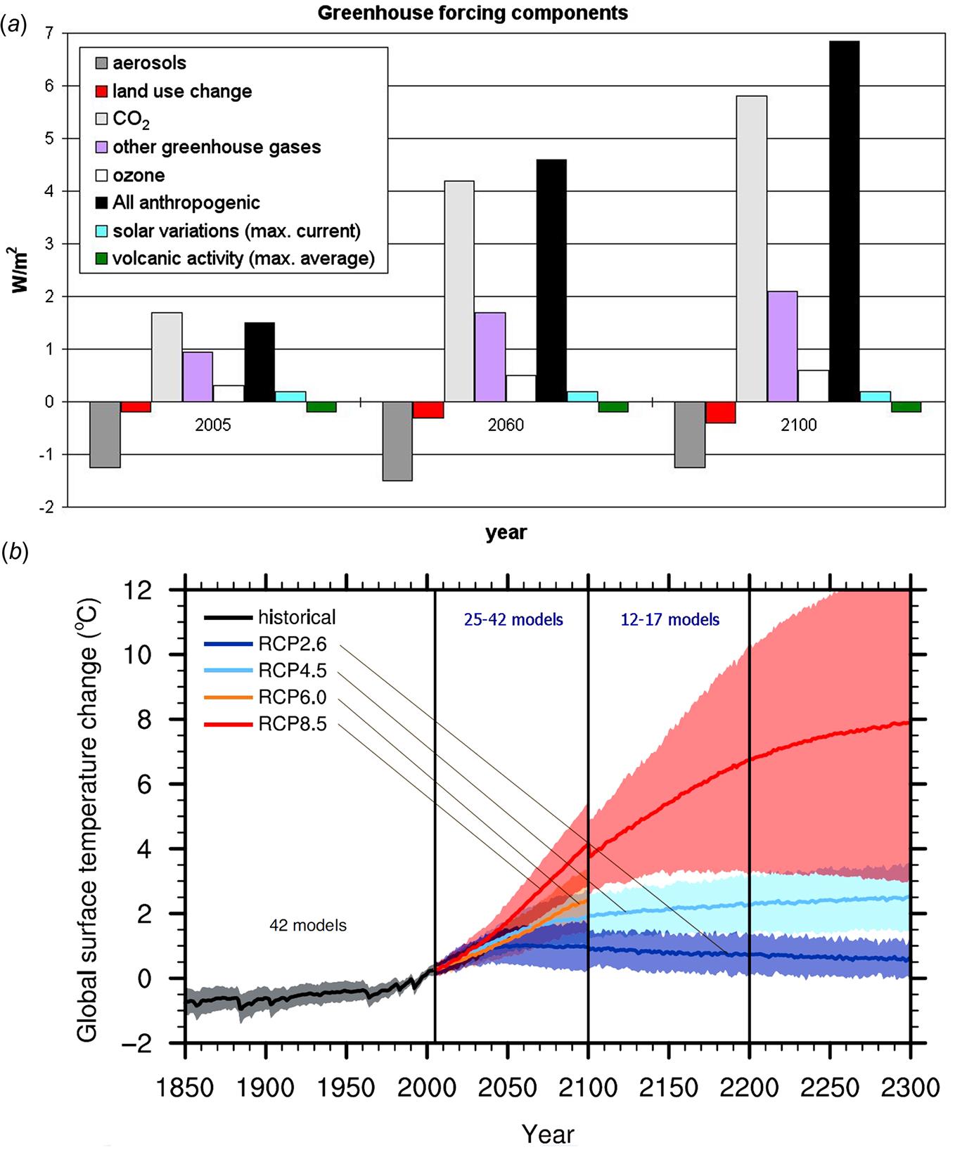
The A1B scenario used in some of the illustrations in this book predicts a 1.6°C global average warming relative to 1990 by 2050 and a 3.0°C warming by 2100. Relative to pre-industrial times, the warming is about 0.75°C higher. The 42 models considered in the 5th IPCC assessment give 2100 over 1995 average temperature increases between 0.6 and 8°C, plus several degrees spread between models, as shown in Fig. 7.16b that for some of the models is further extended to year 2300 (IPCC, 2013).
Greenhouse-warming impacts
Several studies have tried to estimate the damage that may occur as a consequence of the enhanced greenhouse effect. Early studies have concentrated on the damage that may occur in industrialized countries or specifically in North America (Cline, 1992; Frankhauser, 1990; Tol, 1995; Nordhaus, 1994; summaries may be found in IPCC, 1996c). Exceptions are the top-down studies of Hohmeyer (1988) and Ottinger (1991), using rather uninformed guesses regarding starvation deaths from climate change.
The estimation of impacts on agriculture, forestry and ecosystems (including biodiversity changes) particularly depends on the change in natural vegetation zones and local changes in soil moisture and temperatures. Although precise location of the zones within a few hundred kilometers may not be essential, their relative magnitudes would directly affect the impact assessment. As a result, modest confidence can be attached to the impacts predicted, because current climate models have grid dimensions of rarely below 25 km, leading to an accuracy no better than 100 km for the model outputs. Added to this comes all the uncertainty in physical impact assessment, followed by the uncertainty in monetary valuation. All this goes for all the further impact categories that have been identified, such as impacts from extreme weather (heat, cold, storms, flooding, landslides, and droughts) and indirect effects (fires, need to displace people, changed occurrence of vector-borne diseases such as malaria). A detailed account of the current and possible future occurrences of all these impacts may be found in Sørensen (2011), from which the following summary is derived. The first impact to be described is one that the IPCC has largely neglected except for qualitative mention of heat spells, namely the direct health effects of altered temperature. Observed mortality data allow these effects to be estimated rather unambiguously, even if the precise medical causes of changed mortality cannot be pinpointed.
7.3.3.2 Direct health impacts of temperature changes
The impact of extreme temperatures on human survival is rarely a simple relation between high or low temperatures and specific diseases. Ambient temperature may furnish a small push on top of other causes, altering the outcome of a health condition. In this way, ambient temperatures may be a contributing cause for fatal outcome of a variety of diseases, particular in the areas of respiratory and cardiovascular disease and heat failures, myocardial infarction and adverse cerebrovascular conditions, having special affinity to individuals with particular dispositions and health histories. The risk associated with severe frost and its dependence on clothes and shelter is perhaps more well known, and so is the one associated with specific heat-wave episodes that are supposed to become more frequent and/or prolonged in a warmer and less stable climate induced by greenhouse gas emissions (IPCC, 2007b). Basu (2009) notes that the very young (below 4 years) and the old (with a gradual rise accelerating above age 75) are most vulnerable to heat waves.
Temperature changes also have indirect effects through altered requirements for energy management in shelters such as dwellings or workspaces in buildings (costs estimates in Sørensen, 2011). Additional allergy cases would be associated with increased levels of pollen and air pollution due to warming and would occur predominantly at lower latitudes, whereas asthma incidence is highest in humid climates and is expected to be enhanced at higher latitudes (IPCC, 1996a, Chapter 18).
With respect to exceptional upward temperature excursions, the US NRC (2010) presents a US heat-wave duration index defined as the average length (in days) of events. At 2°C average warming, the length index increases by about 8 days in Southern United States and by about 4 days in the Northern States. WHO (2004a) have surveyed the impacts of heat waves but find attribution of death of illness difficult. Epidemiological studies during recent heat-wave incidences are reviewed in Basu (2009). A general relation between maximum daily temperature and mortality has been noted both in Europe and the United States.
Figure 7.17 shows the relation between mortality and daily maximum temperature used as a basis for the calculation discussed below. It is constructed from specific data from a number of European sites (WHO, 2004a), including detailed data for Madrid (Diaz and Santiago, 2003). The inhabitants of Madrid suffer health problems at cold temperatures that are not as low as those causing trouble in most other parts of Europe, while their problems at high temperatures set in at a temperatures higher than in most other European locations. Regional studies have identified several other details of heat-related health impacts. For example, Checkley et al. (2000) finds a doubling of diarrhea cases in Lima (Peru) during an exceptional heat-episode in 1997–98, Ishigami et al. (2008) find 7%–20% elevated mortality per degree warming in a study comprising Budapest, London, and Milano, and Almeida et al. (2010) find about 2% increase in mortality per degree in Lisbon and Oporto. Clearly, the impacts of either cold or hot weather depend on how much time people spent outside at ambient temperatures, and on the quality of the shelter (such as homes, workplaces, and commercial buildings) where they spent the rest of their time. The fact that health problems in cold periods seem higher in Spain than in Norway may not necessarily reflect an adaptation to a certain climate, but could derive from Spanish buildings being less well insulated and otherwise prepared for severe cold spells than those in Norway.

The relative mortality in Fig. 7.17, called the mortality factor, is normalized (choice of unit “1”) in such a way that the Madrid mortality agrees with the observed one. The curves for different locations all have a similar shape, with increased mortality at low and high ambient temperatures, but they are displaced horizontally from each other, by up to about 10°C between Norway and Spain. The one used is an envelope, broadening the bottom part of the curves and using the low-temperature rise of the coldest region and the high-temperature rise of the hottest region. This makes sure that the health impact is not overestimated. The cause of the differences between locations is likely some kind of adaptation, obtained by populations that have lived in a given region for periods exceeding 1000 years. Newcomers usually have different mortality patterns, for many kinds of reasons. It is possible that the correlation between mortality and maximum temperatures averaged over 1 or 2 weeks before the death would be even stronger than the correlation between mortality and just one day’s maximum temperature. For cold spells, one might instead have used minimum temperatures, but these usually differ little from maximum temperatures during winter periods.
The global distribution of January and July daily maximum temperatures for the mid-21st century are shown in Fig. 7.18, based on a high-quality circulation and climate model, the MIHR model of Hasumi and Emori (2004) and emissions from a scenario called “A1B,” one of the 2007 IPCC reference emission scenarios (Meehl et al., 2007). The maximum temperatures are not necessarily representing heat waves, although they occasionally do. Their magnitude and geographical distribution are similar to those found for average temperatures.

The annually averaged global distribution of the change in mortality factor for the mid-21st century, obtained from the daily maximum temperatures exemplified in Fig. 7.18 by use of the relation in Fig. 7.17, is shown in Fig. 7.19.

The changes in mortality factors due to global warming vary quite strongly through the seasons, and Fig. 7.20 shows the monthly results for the difference between the mid-21st century and the pre-industrial mortality factors. As seen, the effects of greenhouse warming are rarely simply beneficial or detrimental, but have seasonal variations representing increases or decreases in mortality. Still, the overall pattern is that of a division of regions of the world into some with predominantly positive effects and other ones with predominantly negative effects. There is excess mortality near the Equator during some parts of the year and reduced mortality at many latitude regions with subtropical and temperate climate, plus some increase in the mortality factor at very high latitudes. However the mortality factors have to be multiplied by the number of people exposed at a given location, and population densities change the picture because they are high at the low and middle latitudes, but low at the very highest latitudes.


The model thus uses UN projected year-2050 population data available for each grid cell, with a modification proposed by Sørensen and Meibom (2000) for city growth, but otherwise based on and maintaining averages from the middle of three United Nations projections for 2050 (CIESIN, 1997; United Nations, 1997, 2010). The total 2050 population is 9.3×10⁹, which is higher than the 8.7×10⁹ used in the IPCC A1B emission scenario, but perhaps more realistic, at least in case there is no major wars or other setbacks. The IPCC scenario is not made on a geographical area-basis and thus cannot be used directly for the type of study undertaken here. The Sørensen–Meibom model used takes actual population data and projects the future development on the basis of demographic and economic development, assuming a gradual shift in lifestyles, which will halt the previous trend toward larger and larger population densities in city centers. Instead, city activities are assumed spreading to neighboring grid cells once the population density exceeds a value of 5000 km−2. Such a spread is in agreement with the average actual developments in many parts of the world, but not with the prestigious increase in high-rise buildings in certain newly rich cities. Because the temperatures in city centers can be 1°C–2°C higher than that outside the cities, the assumptions made in this respect will have an impact of the mortality estimates, probably overlooked by the current coarse-grid climate models.
The model now goes on to multiply the 2050 population by the excess death rate obtained by multiplying current death rates (taken as national figures as given by WRI, 2008) by the 2050 change in mortality factor (for which averages were given in Figs. 7.19 and 7.20). The area of the grid cells entering the geographical-information-system (GIS) calculation to get from the input population density to grid-cell population is for the MIHR model equal to the cosine-corrected latitude increment of 1.121283° times a longitude increment of 1.125°, or 15610.6×cos(j) km2, with j being the latitude angle. When the mortality change in this way is folded with the assumed 2050 population densities, one obtains the predicted number of both additional deaths and avoided deaths shown in Fig. 7.21. The effect of greenhouse warming on the mid-21st century temperature environments is the only one included in this modeling, departing from the current global mortality pattern and adding only this type of modification. There are many other developments that can change and in several cases is known to historically have changed the mortality (medical progress, healthier living or the opposite, etc.), and no attempt has been made to estimate the nature of these other changes from now to year 2050.

The striking conclusion from Fig. 7.21 is that that the numbers of extra lives taken or saved by the greenhouse warming are both very large. Although they are hidden behind medical causes to which deaths are often attributed, due to being only a contributing factor of anything from a few undisclosed percent to the comparatively rare identification as a main cause of death, the statistical approach taken is solid (due to the U-shaped effect shown in Fig. 7.17 being far beyond uncertainty) and the results therefore basically indisputable. The death certificates earlier in use are now being discontinued in many countries (except if criminal causes are suspected), because of their arbitrariness, where the certificate is sometimes signed by a doctor who does not know the deceased and writes say “pneumonia” instead of a more relevant underlying disease that would have been known to a doctor with longer acquaintance with the deceased. In any case multiple causes contributing various percentages to a death are nearly never mentioned in death certificates. Using as here overall mortality data rather than specific causes of death significantly increases the statistical reliability of the study, and at the same time removes the negative influence on the results, that incorrect cause-of-death assignments on death-certificates could otherwise have.
Nearly 4 million people will be affected each year by the climate change brought about by previous greenhouse gas emissions and changes in area use according to the A1B scenario. Of these, 2.2×10⁶ y−1, living in the northern part of the globe plus New Zealand, the Andes and Southern Chile, are people surviving that would have died without the greenhouse warming, and 1.6×10⁶ y−1, living in the Equatorial and southern part of the globe are people that would otherwise have survived but now die. The slightly larger number of deaths avoided by the greenhouse warming according to Fig. 7.21, compared to the number of deaths caused by it, does not allow the interpretation that the two “average out,” as they occur in different regions of the world. Furthermore, from a moral point of view, it is worrisome that the additional deaths occur in countries contributing only little to the greenhouse gas emissions, while the saved deaths occur precisely in the countries most responsible for the greenhouse emissions.
Improvements to the simple model used here would use different mortality factors for every location or at least every region. However, such calculations are not presently possible, because temperature-mortality correlation data have been established only in selected areas (such as the ones mentioned above) and are not globally available. Furthermore, as mentioned, mortality may be influenced by many other factors, which adds uncertainty to use of data collected at even slightly different times. For instance, Donaldson et al. (2003) find that despite an increase in average temperature between 1971 and 1997, the overall mortality decreased in selected countries over the same period.
Another issue to consider in future modeling of the temperature effect is the timing of temperature events influencing mortality. For example, one could look for the correlation between mortality and temperatures a month or a week before each death and compare it with the correlation found between mortality and the temperature at the time of death.
Regarding the level of adaptation to temperature regimes at different locations, it would seem more likely that human populations may adapt to changes in mean temperature, as opposed to adaptation to extreme events.
Bosello et al. (2006) have previously looked at health impacts of warming based on data extrapolated from some specific investigations and they find for 2050 a decrease of deaths from cardiovascular diseases in all regions of the world, totaling 1.76×10⁶; an increase of respiratory diseases causing death in all regions, totaling 0.36×10⁶; and similarly an increase of deaths from diarrhea, totaling 0.49×10⁶. The order of magnitude thus agrees with the present study. However, details appear quite different. The geographical distribution cannot be compared, because Bosello et al. (2006) use aggregated regions with, e.g., India and China lumped together, and they have negative overall impacts only for the Middle East and the “rest of the world,” comprising what is left behind after detailing the “Annex 1” countries (UN jargon for countries classified as industrialized or economies in transition). Other early studies of greenhouse warming impacts by economists have as mentioned concentrated on impacts occurring in the United States (Cline, 1992; Frankhauser, 1990; Nordhaus 1994; Tol, 1995).
7.3.3.3 Impacts on agriculture, silviculture, and ecosystems
One major issue is the impact of climate change on agricultural production. Earlier evaluations (e.g., Hohmeyer, 1988) found food shortage to be the greenhouse impact of highest importance. However, the 1995 IPCC assessment suggested that, in developed countries, farmers will be able to adapt crop choices to the slowly changing climate, and that the impacts will be entirely in the Third World, where farmers will lack the skills needed to adapt. The estimated production loss amounts to 10%–30% of the total global agricultural production (Reilly et al., Chapter 13 in IPCC, 1996a), which would increase the number of people exposed to risk of hunger from the present 640 million to somewhere between 700 and 1000 million (Parry and Rosenzweig, 1993). However, there are also unexploited possibilities for increasing crop yields in developing countries, so the outcome will depend on many factors, including speed of technology transfer and development. The 2nd IPCC assessment expected some 50 million deaths associated with migration (people running away from bad conditions) due to adverse climate events. The following IPCC assessments have added more aspects to the issue and further weakened the early view that warming would imply increased agricultural yields. Hot weather can damage certain crops, and so will dry spells and wildfires, insect attacks will increase, and water supply may become reduced, e.g., for irrigation (Ciais et al., 2005). Desalination of seawater is already in progress in many regions, using either solar energy or still in most cases fossil energy, causing more global warming along with the effort to mitigate its effects.
Fauna adapted to live in areas with a certain climate may try to migrate in order to find new habitats with the climatic conditions they prefer. This may involve displacement by over 1000 km in some cases and may not be possible due to human uses of the intermediate areas, with loss of diversity as a possible outcome (Wright et al., 2009; US NRC, 2010).
In addition to causing warming, ozone may have a direct effect on plant growth (Long et al., 2005; Challinor and Wheeler, 2008). Spruce forests in Sweden seem to be negatively influenced by the shortening of the frost period caused by greenhouse warming (Rammig et al., 2010), and Baltic Sea aquatic plant growth is weakened by changes in oxygen and salinity content in the water (Neumann, 2010). Oxygen is depleted by increased algal growth near shores, and associated cyanobacterial toxins can cause skin rashes and adverse gastrointestinal, respiratory, and allergic reactions (Kite-Powell et al., 2008; Stewart et al., 2006). The many impacts that greenhouse warming can have on agriculture, silviculture, and aquaculture need to be followed closely, but the current estimates of a yield reduction of some 15% already has serious implications for food supply and food prices.
7.3.3.4 Vector-borne diseases
A number of diseases caused by viruses or other microbes are transmitted by insects, called “vectors,” with typical ones being mosquitoes. The plasmodium falciparum parasite and anopheline mosquito varieties involved in the malaria transmission cycle are all sensitive to variations in temperature and humidity, and regions with strong seasonality or dryness in periods of the year crucial for mosquito breeding may experience considerable diminishment of malaria incidence. Other factors are of course lifestyle and technical means such as mosquito nets over beds or wire-netting on window and doors. Models have been constructed for describing the distribution and intensity of malaria transmission under assumptions of various greenhouse warming scenarios (Tanser et al., 2003; Lieshout et al., 2004; Rogers et al., 2002; Bouma, 2003). Current malaria deaths and disabilities (measured in terms of DALY’s, defined as life-shortening in years of not being able to live a normal, meaningful life) are shown in Fig. 7.22. Many attempts to prevent or to heal malaria have been disappointing or have led to drug resistance (notably reducing the usefulness of quinine, chlorochinine, and mefloquine), despite increased understanding of the genetic mechanisms underlying the disease (Olzewski et al., 2010). The earlier IPCC assessments listed spread of malaria to more regions as one of the largest impacts of greenhouse warming, but the actual development during the early 21st century does not support this interpretation, maybe because of increased use of protection and improved living conditions. One should remember that malaria was widespread in Europe a few centuries ago, but largely disappeared along with general socioeconomic development.

Several other vector-borne or parasitic diseases have been monitored by the studies summarized by the IPCC assessments, including helminthiasis, dengue fever, schistosomiasis (bilharziasis), tryponospmiasis, Chagas disease (sleeping sickness), leichmaniasis (black fever), lymphatic filariasis (elephantiasis), and onchocerciatis (river blindness). All of these are considered to be influenced by greenhouse warming (Weaver et al., 2010; Hales et al., 2002; WHO, 2004b; Mathers and Loncar, 2006). Overall, considering the expected economic development in the regions currently affected, the World Health Organization expects these diseases to diminish in importance over the next decades (WHO, 2008, 2010).
7.3.3.5 Extreme events
Already at present, an increased frequency and severity of extreme events with possible connection to greenhouse warming (floods, landslides, storms, droughts, and fires) has been noted and has influenced insurance premiums. Some climate models claim to predict such increases (see discussion in Sillmann et al., 2013), but basically, the mechanism for many of these events would seem to involve interaction between atmospheric motion on small and large scales, which is not covered by the models used that has to omit local eddy circulation and chaotic air motion, as explained in section 2.3.1. The development in number of floods in two severity classes globally is shown in Fig. 7.23, death and disability caused by fires in Fig. 7.24, and an overview of some important natural and manmade extreme events is given in Fig. 7.25. There is no easy way to estimate the precise future frequency of any of these events, but global warming seems generally to lower the stability of climates.


7.3.3.6 Valuation of greenhouse warming impacts
As discussed earlier in this chapter, monetizing the physical impacts identified can be quite ambiguous due to the limitations of the concept of a “statistical value of life.” The study presented above predicts that additional deaths caused by greenhouse warming will predominantly occur in regions of low income, which in some studies has lead to setting the value of a life lost at a lower level than for the regions where lives according to the present study are abundantly being saved by the greenhouse warming. Clearly a number of ethical issues are involved in estimating the impacts of human activities carried out by precisely the group of people that stands to benefit from the green-house gas pollution, while negative effects are accumulated in populations with less affluence and a lesser possibility to control or mitigate the impacts.
Impacts on human societies and the natural environment involve health issues (deaths and DALYs), economic issues, degrading the environment, and affecting biological diversity. The key problem of valuing human lives lost is here handled by introduction of a “statistical value of life,” and Table 7.2 summarizes the studies made initiated by the 1995 European Commission study “ExternE” and several follow-up studies (US EPA, 2015; Viscusi and Aldi, 2003). The columns termed “European Standards” are the ExternE valuation expressed in € or US $ without correcting the amount for later inflation, and the two last columns give a purchasing power parity (PPP) and a GDP-adjusted conversion. The order of magnitude difference between the three methods of evaluating explains many of the disparities found in the literature and leaves a choice between evaluating lost lives everywhere by the standards of the rich countries or by the PPP measure. The GDP-adjusted valuation of statistical lives is clearly unacceptable.
Table 7.2
Valuation assumptions used in Table 7.3 and several of the further life-cycle studies in this chapter
| Valuation Method: | European Standards | PPP-Adjusteda | GDP-Adjusteda | |
| Health Effect/Valuation | US $ | € | € | € |
| Induced death (SVL) | 3 250 000 | 2 600 000 | 1 040 000 | 26 000 |
| Disability-adjusted life-shortening (DALY) | 81 250 | 65 000 | 26 000 | 650 |
| Derived from components: | ||||
| Respiratory hospital admission | 8250 | 6600 | ||
| Emergency room visits | 233 | 186 | ||
| Bronchitis | 173 | 138 | ||
| One day activity restricted | 78 | 62 | ||
| Asthma attack | 39 | 31 | ||
| One day with symptoms | 8 | 6 | ||

The “European Standards” derive from a study by the European Commission (1995b). The purchasing power parity (PPP) and the GDP-adjusted values are derived with use of Wikipedia (2010). See details in Sørensen (2011). Year 2011 exchange rate is used.
aUsing a purchasing power parity (PPP) adjustment by a factor of 2.5 relative to European standards of salaries and market prices for consumer goods. The GDP-adjustment is made by scaling the valuation by an average gross domestic product ratio of 100, the approximate average ratio found between central African and European Union countries (Wikipedia, 2010). The purpose of presenting European and least developed valuations is to provide practical upper and lower bounds for LCA calculations, without including the absolute highs or lows for particular individuals.
Based on these rules of evaluation, the greenhouse warming effects identified above have been monetized. The results are presented in Table 7.3 and Fig. 7.26 (Sørensen, 2011), where an estimate for the entire 21st century impact is obtained by multiplying the results for the mid-century by 100. It is seen that the large impact contributors are the decrease in food production (agriculture and fisheries) and the direct temperature impact on health, positive or negative. The temperature impact was deemed minor in previous IPCC estimates, and the malaria and other vector-transmitted diseases that dominated the previous IPCC estimates (see Sørensen, 2010) are in Table 7.3 not quantified, because the current stance is that they may not play any significant role a few decades ahead. Despite the large direct temperature impacts of both signs, the sum of all impacts included is negative and large, although it only equals about a third of the impacts found based on the previous IPCC assessment (Sørensen, 2010). As also discussed above, the presence of two large, partly canceling contributions does not diminish the human suffering from the negative part, because they occur in different regions of the world.
Table 7.3
Estimated global warming impacts during the 21st century, based on IPCC scenario A1B for the mid-21st century, multiplied by 100
| Impact Description: | Valuation (1012 €) | ||
| M=106, G=109. Type of Valuation Parameters: | EU-Standards | PPP-Adjusted | GNP-Adjusted |
| Decrease in agricultural production (~15% before adaptation)→higher food prices, shifts to other crops→possible starvation. Population at risk: 0.6 G→1 G, with ~ 0.1 G extra deaths over 21st century), | −260 | −104 | −2.6 |
| Reduced forestry output (as in Kuemmel et al., 1997). Impact curbed by substitution. | −4 | −1.6 | −0.4 |
| Decrease in fishery output (probably more than 15%). Ocean and aquiculture production more important in future implying maybe 40 M extra deaths. | −104 | −42 | −1.0 |
| More extreme events: floods (~20% increase, 0.86→1.03 M deaths, 14 G→17 G dislocations at 0.1 DALY) | −20 | −9 | −4 |
| More extreme events: draughts (~20% increase, 0.07→0.08 M deaths, 7.0 G→8.4 G affected at 0.01 DALY) | −1 | −0.4 | −0.01 |
| More extreme events: fires (~20% increase for the 50% of the total considered climate-related, 31→34 M deaths, 0.57 G→0.69 G DALY’s) | −16 | −9 | −3.2 |
| More extreme events: storms (~20% increase, 1.57→1.89 M deaths, 0.5 G→0.6 G affected at 0.01 DALY) | −1 | −0.4 | −0.01 |
| Unspecific human migration in response to environmental & social impacts of warming (0.3 G affected) | −4 | −1.4 | −0.04 |
| Malaria (presently 0.9 M deaths/y and 35 M DALY/y (with 17 G infected). Estimates for 2050 are 3–5 times less, clouding −8% to +16% change due to warming) | ? | ? | ? |
| Dengue fever and tropical-cluster diseases. Remarks made for malaria apply, but values are 3–6 times less | ? | ? | ? |
| Positive health effects of higher temperatures and fewer cold-spells (220 M deaths avoided) | +572 | +297 | +119 |
| Negative health effects of higher temperatures and more heat-waves (160 M more deaths) | −416 | −224 | −87 |
| Increase in skin-cancer, asthma and allergy cases | −6 | −5 | −4 |
| Loss of species, ecosystem damage, freshwater problems, insect increase, etc. (as in Kuemmel et al., 1997) | −50 | −20 | −0.5 |
| Loss of tourism, socioeconomic adaptation problems | ? | ? | ? |
| Total of valuated impacts (highly uncertain) | −310 | −120 | +16 |

Source: From Sørensen (2011) used with permission.

Estimating greenhouse-warming externalities for fuel combustion
In assessing the life-cycle impacts of specific energy technologies, the impact of the greenhouse gas emissions found above must be translated into externalities per unit of energy conversion. The 2nd IPCC report discussed an issue called grandfathering, concerned with whether the cost of total greenhouse impacts should only be imposed as an economic burden on future emissions, or distributed evenly over all emissions, including past ones that could not be changed. The range of estimates with and without grandfathering from the 2nd IPCC assessment is exhibited in Table 7.4, because they are used in some of the LCA assessments below. As mentioned, also aerosol emissions are smaller in the recent IPCC reports than in the earlier one, affecting the analyses made on the earlier basis.
Table 7.4
Different methods for describing greenhouse-warming impact, using the IPCC A1B scenario with and without grandfathering, and a scenario with 1.5°C warming 2000–2100
| Greenhouse Warming Impacts | Estimate I IPCC A1B, Grandfathering | Estimate II IPCC A1B, No Grandfathering | Estimate III Sørensen (2008) ΔT≤1.5°C Scenario, Grandfathering |
| Cause (emission assumptions): | All CO2 emissions 1990–2060: | All CO2 emissions 1765–2060: | CO2 allowance 2000–2100: |
| Effect (full 21st century cost): | 310×1012 € (Table 7.3) | 310×1012 € (Table 7.3) | 187×1012 € (scaled) |
| Specific externality: | 0.38 €/kg C=0.10 €/kg CO2 | 0.27 €/kg C=0.07 €/kg CO2 | 0.38 €/kg C=0.10 €/kg CO2 |