
Thus, infrared radiation to space is little affected by the presence of an aerosol layer, relative to the influence on the transmission of visible light. In Fig. 2.99, an Llw scale is added at the top, and curves representing the long-wavelength radiation to space are drawn (thin lines) for different values of the surface temperature, Ts, i.e., the Planck radiation temperature of the upward radiation spectrum [cf. (2.3)]. The optical aerosol thickness at present is believed to be around 0.1. The figure indicates that in order to decrease the average surface temperature by one degree, the aerosol content would have to be increased by a factor of 1.5–2.0. For the average residence time around 15 days mentioned for atmospheric particles in section 2.3.1, the particle emission, which increases the atmospheric load by a factor of two, can be taken as twice the present level. Thus, if 20% of the emissions (including emission of gases that later form particles) at present are of anthropogenic origin, then a doubling of the total amount would require a sixfold increase of the anthropogenic emissions.
The newest climate model calculations mentioned below under “carbon dioxide” all include a model for aerosol content in the atmosphere.
2.4.2.7 Carbon dioxide
Gaseous emissions into the atmosphere may entail environmental side-effects and may affect human health. Such pollution has been demonstrated, for example, in connection with sulfur oxides from fossil fuel combustion and with photochemical smog. However, trace gases may also interfere directly with climate, by altering components of the radiation fluxes. As can be seen from Fig. 2.40, H2O and CO2 are very important absorbers in the infrared wavelength region, particularly for wavelengths above 10−5 m, where the peak of the long-wavelength radiation to space is situated. It is thus to be expected that an increase in the atmospheric content of these absorbers will lead to a higher temperature in the troposphere as well as on the Earth’s surface. The present content of CO2 is already big enough to imply a nearly total absorption at λ=1.5×10⁻⁵ m. It is therefore unlikely that even a dramatic increase in CO2 could have consequences similar to the addition of a small amount of NH3 (temperature changes globally averaging something of the order of 10°C or more), discussed earlier in this section. However, a temperature change of just 1 or 2° globally may have serious effects on climate, particularly if the local temperature change is amplified in sensitive regions, such as the polar regions.
As shown in Fig. 2.92, a little over half of the anthropogenic CO2 emissions are accumulating in the atmosphere, but it is difficult to determine precisely the magnitude of future emissions that would lead to a specific temperature increase, owing to the non-linear absorption response at the specific radiation wavelengths characterizing each gas contributing to greenhouse warming (cf. Fig. 2.40).
Numerous calculations estimating the climatic effects of doubling the atmospheric CO2 content have been performed over the years. An early model by Manabe and Wetherald (1967) used a global average one-dimensional (height) temperature distribution, taking into account both the changes in radiation components and the change in the turbulent (convective) fluxes from the surface, as a function of CO2 content. Assuming a fixed relative humidity and cloudiness, a doubling of the CO2 concentration in this calculation implied a temperature increase at the Earth’s surface amounting to 2.4 K. A later three-dimensional equilibrium model used by Manabe and Wetherald (1975) employed the techniques described in section 2.3.1, but with the idealized topography discussed in section 2.3.2 in connection with the joint ocean–atmosphere model of the same authors. No seasonal variations of radiation were considered in that calculation, with no oceanic heat transport, and the cloud cover was fixed at 0.5. Test computations starting with substantially different initial conditions gave equilibrium temperature distributions that concurred with each other to better than about 1 K. Figure 2.100 shows the hemispherical longitude averages of temperature for the calculation with CO2 content doubled, minus the corresponding temperatures for a reference calculation (CO2 mixing ratio 4.56×10⁻⁷ by mass). In the stratosphere, the doubled CO2 content leads to a net cooling, while the troposphere is heated. The temperature at mid-heights is increased by about 3 K, while the surface temperature is increased by 2–3 K, except in the polar region, where the temperature increases by up to 10 K. The sensitivity of the polar region is associated with the possibility of large albedo changes, primarily connected with ice melting. The model predicts a poleward movement of the border of the ice cap by about 10°, plus a reduction in the thickness of snow cover. The latter is due to reduced snowfall (in the polar region), while the total amount of precipitation increases at all latitudes, as a result of doubling CO2. For this reason, the latent heat upward flux (evaporation) increases significantly, and the warming of the troposphere by a greenhouse effect is due to the combined absorption of radiation by water vapor and CO2. The effective temperature T0 of the entire Earth–atmosphere system is increased by roughly 0.6 K, but the authors warn that the strong interconnection between the CO2 cycle and the hydrological cycle that the model has indicated may necessitate the inclusion of a predictive equation for the cloud cover in their model.

Finally, Fig. 2.101 gives the results of a recent modeling effort using a grid with spatial resolution 2.5°×3.75° combined with 19 atmospheric height levels and 20 oceanic depth levels (Mitchell et al., 1995; Mitchell and Johns, 1997). The model is transient, starting with realistic data from about the year 1860 and following the development under conditions of changing CO2 emissions as well as taking into account the sulfate aerosol negative forcing. Model output for the present era substantially agrees with observed data, and Fig. 2.101 shows the geographical distribution of calculated change between surface temperatures around 2055 and those characterizing the 1990s for each season, averaged over period of 10 years.


Compared to the earlier calculation, the only significant change is the cooling effect of particles in the atmosphere, which is strong at present and in the near future (giving a very complex temperature modification pattern), but diminishes in importance toward the end of the period because of assumed reductions in sulfate aerosol emissions from power plants and other activities, as environmental regulation introduced in many countries today is making itself felt globally. The average warming from the doubled CO2 is about 2.5°C.
There is a continued effort to include more and more realistic effects in the climate simulation models. The effort includes differentiating between different residence times of different greenhouse gases (rather that lumping them together as an “effective CO2 emission”); improving modeling of cloud and water vapor in general, of oceanic transport, and of transfer of heat and particles between oceans and atmosphere; and, of course, refining the grid resolution and accuracy of topography.
Support for the correctness of the calculated persistence in the atmosphere of greenhouse gases has recently come from the analysis of a climatic change that occurred 55 million years ago and that is interpreted as having been caused by sudden release of methane from sedimentary hydrides. The residence time found by the sediment core study is 120 000 years (Norris and Röhl, 1999).
It is not the intention here to give an extensive list of possibilities for human interference with climate. In brief, it may be stated that life, and in particular human life, is sensitive to even very small changes in certain critical elements. Among these, a well-established case is that of ultraviolet radiation penetration to the surface, which, as discussed in section 2.3.1, depends on the presence of definite trace gases in the stratosphere (see Fig. 2.38). In particular, it has been suggested that the ozone concentration may be very sensitive to various human activities, such as aircraft combustion products (see, for example, Alyea et al., 1975), chlorofluoromethanes (see, for example, Wofsy et al., 1975), and nitrous oxide, N2O, from increased use of fertilizers in agriculture (Johnston, 1977) (cf. section 2.4.1). In the two latter cases, the gases in question are very inert in the troposphere, but may become catalysts for chemical processes in the stratosphere by which ozone is depleted. The modeling of these changes, and their induced modifications of the radiative spectrum (Cutchis, 1974), was one of the first climate calculations undertaken. It involves a detailed knowledge of the chemistry and photochemistry of the atmosphere, together with the general atmospheric models describing the circulation and other physical processes, in particular the mixing and diffusion processes between the stratosphere and the lower atmosphere.
As a result of these calculations, international agreements on the reduction of emissions affecting the ozone content in the atmosphere have been reached, and similar agreements may theoretically be forthcoming regarding the curbing of greenhouse gas emissions. The very substantial economic implications involved are discussed in Chapters 7 and 8.
2.5 Inclusion of non-radiative energy flows
2.5.1 Vertical transport in the atmosphere
If the transport of sensible or latent energy is governed by the gradients of temperature and humidity, it may be described by the diffusion equation (see, for example, Sellers, 1965)
(2.28)
where k is the diffusion coefficient and the z-axis is in the vertical direction. Considering a quasi-stationary situation (the partial derivatives of T with respect to time t as well as with respect to horizontal directions x and y being considered negligible), (2.28) may be integrated to give
(2.29)
The change in stored sensible heat in a small volume dx dy dz close to the ground is
and the sensible heat flux per unit area is thus
Insertion of this into (2.28) explains the form of the constant used on the right-hand side of (2.29).
The vertical transport of water vapor through the laminar boundary layer may also be taken as a diffusion-type process and is given by the equation analogous to (2.29),
(2.30)
where q is the specific humidity. The molecular diffusion coefficient in air is of the order of k=2×10⁻⁵ m2 s−1.
Considering the vertical change in the horizontal velocity u of the air, the expression analogous to (2.29) or (2.30),
(2.31)
represents the shearing stress acting on the ground (or more generally on a horizontal unit area). τ has the dimension of force per unit area or pressure.
Above the laminar boundary layer, transport usually takes place by turbulent convection. The mass motion may be considered as consisting of overlaying eddies of varying size, eventually superimposed on a laminar flow. The fact that laminar flow is, in general, horizontal or nearly horizontal near the ground implies that all vertical transport is related to eddy motion.
It is now assumed (Rossby, 1932) that the expressions (2.29)–(2.31), based on molecular diffusion theory, can also be applied in the region of turbulent motion, provided that the coefficient k is given an effective value. This eddy diffusion parameter is no longer constant. It will depend on the quantity being transported and on the velocity field of the atmosphere, i.e., k will be a time-dependent function of the height z. The picture of turbulent transport given here is equivalent to the mixing length formulation used in the discussion in section 2.1.1 of convective transport in stellar atmospheres. The eddy diffusion parameter k is related to the mixing length l by
If the temperature profile is approximately adiabatic,
(2.32)
(P is pressure, cV is the heat capacity at constant volume), then it has been suggested that the mixing length be taken as proportional to or at least a linear function of z,
or
(2.33)
where κ close to 0.4 is von Kármáns constant (Prandtl, 1932). Using (2.33) together with the assumption that the shearing stress τ (2.31) is independent of z within the stable atmospheric layer, where the temperature gradient has been assumed to correspond to adiabaticity, then the horizontal velocity varies with height according to
(2.34)
The lower limit of integration, z0, is the height of the laminar boundary layer, for which the velocity u becomes zero if the first expression (2.33) for l is used, whereas for the second expression the velocity u becomes zero at the ground, z=0. None of the expressions can be rigorously correct, since the second one, which gives the correct boundary condition u(z=0)=0, also predicts eddies that extend to the ground, l(z=0)≠0, in contradiction to the basic assumptions regarding the laminar boundary layer. The first expression correctly predicts l(0)=0, but cannot be used to estimate u if z ![]() z0. The coefficient (τ/ρ)1/2 has the dimension of velocity and is often referred to as the friction velocity.
z0. The coefficient (τ/ρ)1/2 has the dimension of velocity and is often referred to as the friction velocity.
If the eddy diffusion parameter k is left as a function of z [to be determined empirically rather than using (2.33)], and the heat flux Esens is regarded as independent of z, then (2.29) may be integrated,
According to Budyko (1974), the integral appearing on the left-hand side depends little on z, in contrast to k, so that the expression offers an empirical method of determining ![]() from temperature measurements. A similar expression for
from temperature measurements. A similar expression for ![]() may be found from (2.30), again replacing the molecular diffusion coefficient k by the eddy diffusion parameter as a function of z.
may be found from (2.30), again replacing the molecular diffusion coefficient k by the eddy diffusion parameter as a function of z.
2.5.1.1 Water transport
The transport of water vapor through the lower part of the atmosphere may be described by equation (2.30), which may be read as an expression of the potential evaporation from a “wet surface” (i.e., a surface of moisture exceeding the above-mentioned “critical” value), depending on the distribution of humidity q in the air above the surface, and on the diffusion coefficient k(z), which again may depend on the wind velocity, etc.,
(2.35)
Within the laminar boundary layer, k may be considered constant, but in the turbulent layer, k varies. If the integral
can be considered as constant (Budyko, 1974), an integration of (2.35) shows that e varies linearly with the specific humidity q at some height z above the surface. On the other hand, if k is identified with the diffusion coefficient for horizontal wind velocity u (2.31), one obtains, similarly to (2.34),
and
(2.36)
Several expressions of this structure or similar ones have been compared with measurements, where they are found to agree overall but not in specific detail (see, for example, Sellers, 1965; Sørensen, 1975).
The evaporation from ocean surfaces is not independent of the occurrence of waves. At high wind speeds, surface tension is no longer able to hold the water surface together, and spray droplets are ejected into the atmosphere (whitecaps). Some of these droplets evaporate before they fall back into the sea, thereby providing a source of vapor that does not follow the diffusion formulae given above.
Condensation of water vapor in the atmosphere may take place whenever the vapor pressure of water exceeds that of saturation at the prevailing conditions. However, if no condensation nuclei are present, the vapor may become supersaturated. One source of condensation nuclei that is of particular importance over oceans is the salt particles left over from the spray droplets discussed above, after the evaporation of the water. Typically, the mass of these salt particles is so small that gravitation can be disregarded, and the salt particles may remain suspended in the atmosphere for a considerable length of time. Other particles of suitable size and structure serve equally well as condensation nuclei, and globally the sea-salt spray particles do not dominate the condensation processes (Junge, 1963).
2.5.1.2 The disposition of water and heat in soils
The penetration of water into soil and the movement of ground water depend strongly on local conditions, such as the sequence of soil types. Underground aquifers may transport water at moderate velocities, but the average turnover time even in the regions of active exchange is very slow, 200–300 years, as estimated from Fig. 2.65.
The ability of soils to store heat absorbed from solar radiation depends on the heat capacity of the soil, which may be written
(2.37)
in terms of the heat capacity of dry soil (![]() typically in the range 2.0–2.5×10⁶ J m−3 K−1) and of water [Cw≈4.2×10⁶ J m−3 K−1 or roughly half of this value for ice (frozen soil)]. The mixing ratios (by volume) ms and mw are much more variable. For soils with different air content, ms may be 0.2–0.6 (low for peat, medium for clay, and high for sand). The moisture content mw spans the range from zero to the volume fraction otherwise occupied by air, ma (equal to about 0.4 for clay and sand, but 0.9 for peat) (Sellers, 1965). In temperate climates an average value of mw for the upper soil layer is around 0.16 (Geiger, 1961).
typically in the range 2.0–2.5×10⁶ J m−3 K−1) and of water [Cw≈4.2×10⁶ J m−3 K−1 or roughly half of this value for ice (frozen soil)]. The mixing ratios (by volume) ms and mw are much more variable. For soils with different air content, ms may be 0.2–0.6 (low for peat, medium for clay, and high for sand). The moisture content mw spans the range from zero to the volume fraction otherwise occupied by air, ma (equal to about 0.4 for clay and sand, but 0.9 for peat) (Sellers, 1965). In temperate climates an average value of mw for the upper soil layer is around 0.16 (Geiger, 1961).
Since the absorption of radiation takes place at the soil surface, the storage of heat depends on the competition between downward transport and long-wavelength re-radiation plus evapotranspiration and convective transfer. The thermal conductivity of the soil, λ(z), is defined as the ratio between the rate of heat flow and the temperature gradient, at a given depth z,
(2.38)
(Note that by the sign convention previously adopted, z is negative below the soil surface.) Figure 2.102 gives a rough idea of the dependence of λ on the moisture content for different soil types.

If the downward heat transport can be treated as a diffusion process, equation (2.28) is valid. Taking the partial derivative of (2.38) with respect to depth (−z), and assuming that k and λ are independent of z (homogeneous soil),
Together with the heat transport equation
(cf. section 2.5.2; in the absence of heat sources, heat sinks, and a fluid velocity in the soil), this implies the relation
(2.39)
Figure 2.103 shows an example of the variation in the monthly average temperature as a function of depth in the soil. The time variation diminishes with increasing depth, and the occurrence of the maximum and the minimum is increasingly delayed. These features are direct consequences of the diffusion approach, as one can easily see, for example, by assuming a periodic temperature variation at the surface (Carslaw and Jaeger, 1959),
(2.40)

With this boundary condition, (2.28) can be satisfied by
(2.41)
 (2.41)
and the corresponding heat flux is from (2.38)
(2.42)
 (2.42)
The amplitude of the varying part of the temperature is seen from (2.41) to drop exponentially with depth (−z), as the heat flux (2.42) drops to zero. For a fixed depth, z, the maximum and minimum occur at a time that is delayed proportional to |z|, with the proportionality factor ![]() . The maximum heat flux is further delayed by one-eighth of the cycle period (also at the surface).
. The maximum heat flux is further delayed by one-eighth of the cycle period (also at the surface).
The approximation (2.40) can be used to describe the daily as well as the seasonal variations in T and Ez. For the daily cycle, the surface temperature is maximum sometime between 1200 and 1400 h. This temperature peak starts to move downward, but the highest flux away from the surface is not reached until 3 h later, according to (2.42). While the temperature peak is still moving down, the heat flux at the surface changes sign some 9 h after the peak, i.e., in the late evening. Next morning, 3 h before the peak temperature, the heat flux again changes sign and becomes a downward flux. Of course, the strict sine variation may only be expected at equinoxes.
2.5.1.3 Geothermal heat fluxes
In the above discussion, the heat flux of non-solar origin, coming from the interior of the Earth, has been neglected. This is generally permissible, since the average heat flux from the interior is only of the order of 3×10¹² W, or about 8×10⁻² W m−2. Locally, in regions of volcanoes, hot springs, etc., the geothermal heat fluxes may be much larger. However, it has been estimated that the heat transfer through the Earth’s surface by volcanic activity contributes only less than 1% of the average flux (Gutenberg, 1959). Equally small or smaller is the amount of heat transmitted by seismic waves, and most of this energy does not contribute any flux through the surface.
Although the distribution of heat generation within the solid Earth is not directly measurable, it may be estimated from assumptions on the composition of various layers of the Earth’s interior (cf. Lewis, 1974, and Fig. 2.11). Thus, one finds that most of the heat generation takes place within the rocks present in the Earth’s crust. The source of heat is the decay of radioactive elements, chiefly potassium, uranium, and thorium. The estimated rate of generation (see, for example, Gutenberg, 1959) is roughly of the same order of magnitude as the outward heat flux through the surface, although there is considerable uncertainty about this.
It is believed that the temperature gradient is positive inward (but of varying magnitude) all the way to the center, so that the direction of heat transport is predominantly outward, with possible exceptions in regions of convection or other mass movement.
A more detailed discussion of the nature of the geothermal energy flux is deferred to section 3.4.2.
Temperature gradients also exist in the oceans, but it will become clear that they are primarily maintained not by the heat flux from the Earth’s interior, but by extraterrestrial solar radiation coupled with conditions in the atmosphere and in the surface layers of the continents.
2.5.1.4 Momentum exchange processes between atmosphere and oceans
The mixing and sinking processes sketched above constitute one of the two sources of oceanic circulation. The other one is the momentum exchange between the atmospheric circulation (winds) and the oceans. The interaction between wind and water is complex, because a large fraction of the kinetic energy is transformed into wave motion rather than directly into currents. Although the roughness length over water [z0 of (2.33), (2.34)] is very small, a strong wind is capable of raising waves to a height of about 10 m.
The wind stress acting on the ocean surface may be taken from (2.33),
(2.43)
where ρa is the density of air, κ is von Karman’s constant, and z1 is a reference height. When the height variation of the horizontal wind velocity V is logarithmic as in (2.34), τ is independent of height. This is true for the lower part of the turbulent layer (the Prandtl layer), within which z1 must be taken, and the value of τ found in this way will remain constant through the laminar boundary layer, i.e., the force exerted on the ocean surface can be determined from measurements in a height z1 of, say, 10 m.
However, the approach may be complicated by the motion of the water surface. If waves are propagating along the water surface in the direction of the wind, one may argue that the stress should be proportional to the square of the relative velocity (V−Uw)2, where Uw is the wave velocity, rather than to the square of V alone. Further, the roughness parameter z0 may no longer be a constant, but may depend on the wave velocity as well as on the wave amplitude. Given that the waves are formed as a result of the wind stress τ, this implies a coupled phenomenon, in which τ initiates wave motion, which again modifies τ as a result of a changed surface friction, etc. There is experimental evidence to suggest that z0 is nearly constant except for the lowest wind velocities (and equal to about 6×10⁻³ m; Sverdrup, 1957).
The mechanism by which the surface stress creates waves is not known in detail, nor is the distribution on waves and currents of the energy received by the ocean from the winds, or any subsequent transfer (Pond, 1971). Waves may be defined as motion in which the average position of matter (the water “particles”) is unchanged, whereas currents do transport matter. This may also be viewed as a difference in scale. Waves play a minor role in the atmosphere, but are important in the hydrosphere, particularly in the upper water layers, but also as internal waves. The reason is, of course, the higher density of water, which allows substantial potential energy changes to be caused by modest lifting heights.
2.5.2 Circulation modeling
2.5.2.1 The basic equations in terms of time-averaged variables
As outlined in section 2.3, the averaging procedure leading to (2.23) may now be applied to the general Eulerian equation of transport, for any relevant quantity A,
(2.44)
This equation states that the change in A within a given volume, per unit time, is due to gains from external sources, SA, minus the macroscopic and molecular outflow (divergence terms). The macroscopic outflow is due to the velocity field v, and the microscopic transport is described by a vector sA, the components of which give the transport by molecular processes in the directions of the co-ordinate axes.
Applying the definitions (2.21)–(2.23), the time-averaged version of (2.44) becomes
(2.45)
If A is taken as unity, (2.44) becomes the equation of continuity (of mass),
(2.46)
The density-averaging method is essential for obtaining the same form as for the instantaneous values. If A is taken as a component of the velocity vector, (2.45) becomes [with utilization of (2.46)]
(2.47)
The sources of velocity are the external forces Fext (gravitational and Coriolis forces), and the molecular transfer of velocity (or momentum) is given in terms of the derivatives of the stress tensor τij,
where P is the thermodynamic pressure, η and η′ are the kinematic and volume viscosities, *and δij is the Kronecker delta (Hinze, 1975). In the last term on the left-hand side of (2.47), the divergence operator ![]() is supposed to act on all three factors
is supposed to act on all three factors ![]() following.
following.
It is clear from the equation of motion (2.47) that the large-scale motion of the atmosphere, v*, cannot generally be described by an equation that depends on only averaged quantities (for a discussion of early attempts to achieve such a description, see Lorenz, 1967). The divergence term on the left-hand side describes the influence of small-scale turbulent motion on the large-scale motion. It is usually referred to as the eddy transport term.
Apart from the well-known pressure gradient term, the contributions from the stress tensor describe the molecular friction forces. These may be important for calculations of energy transformations, but are often left out in calculations of general circulation (Wilson and Matthews, 1971). According to Boussinesq (1877), it may be possible to approximate the eddy transport term by an expression of the same form as the dynamic viscosity term [see (2.60)], introducing an effective “eddy viscosity” parameter similar to the parameter k considered above in connection with the turbulent transport of heat from the Earth’s surface to the boundary layer [the Prandtl layer, extending about 50 m above the laminar boundary layer and defined by an approximately constant shear stress τ in expressions like (2.34)].
The difference between the scales of vertical and horizontal motion makes it convenient to define separate velocities w and V,
and split the equation of motion (2.47) into a horizontal part,
(2.48)
and a vertical part, which, as mentioned, can be approximated by the hydrostatic equation,
(2.49)
In (2.48), the molecular friction forces have been left out, and only the vertical derivative is kept in the eddy term. This term thus describes a turbulent friction, by which eddy motion reduces the horizontal average wind velocity V*. The last term in (2.48) is due to the Coriolis force, and
where Ω is the angular velocity of the Earth’s rotation and ϕ is the latitude.
As a lowest-order approximation to the solution of (2.48), all the terms on the left-hand side may be neglected. The resulting horizontal average wind is called the geostrophic wind, and it depends on only the pressure gradient at a given height and a given geographical position. The smallness of the left-hand terms in (2.48), relative to the terms on the right-hand side, is, of course, an empirical relationship found specifically in the Earth’s atmosphere. It may not be valid for other flow systems.
The large-scale horizontal wind approaches the geostrophic approximation when neither height nor latitude is too small. At lower heights the turbulent friction term becomes more important (up to about 1000 m), and at low latitudes the Coriolis term becomes smaller, so that it no longer dominates over the terms involving local time and space derivatives.
In analogy to (2.47), the averaging procedure may now be applied to the general transport equation for some scalar quantity, such as the mixing ratio for some minor constituent of the atmosphere. Equation (2.47) then becomes
(2.50)
The source term on the right-hand side indicates whether the substance in question is created or lost, for example, by phase changes or chemical reactions. SA will, in general, depend on all the state variables of the atmosphere, the air velocity, and the mixing ratios for other constituents. In an approximate manner, the source term may be taken to depend only on the average values of its parameters (Wilson and Matthews, 1971),
The ideal gas approximation to the equation of state for the air reads, in averaged form,
(2.51)
where ℜ/μ ≅ 280 m2 s−2 K−1 up to a height z of about 90 km, above which level the molecular weight drops quickly. Eventually, a correction depending on humidity may be incorporated into (2.51).
Temperature is often replaced by a variable called the potential temperature, defined by
(2.52)
where the constant P0 is usually taken as the standard sea-level pressure (105 N m−2). The significance of the potential temperature is that it is constant during processes that do not change entropy. Figure 2.104 shows an example of latitude variations of θ* and T* based on the same data.

The first law of thermodynamics states that the change in internal energy per unit mass is given by
(2.53)
where Q is the amount of heat added to the system (an air parcel of unit mass) per second. As in (2.48), the molecular friction (which also produces heat) will be left out. From the definition of specific entropy s, one obtains
and by introducing the potential temperature (2.52),
Inserting this into (2.53), the time derivative of θ is obtained,
This is the source term to be entered on the right-hand side of the expression (2.50) for the averaged potential temperature,
(2.54)
Again the last term on the left-hand side describes an amount of heat lost from a given volume by small-scale vertical eddy motion. The external heat sources are radiation and, according to the implicit way of treating latent heat, the heat of condensation of water vapor (plus possibly other phase change contributions),
where R is the amount of heat added to a unit volume by radiation and C is the contribution from condensation processes.
For the approximations considered, a complete set of equations for the atmosphere is constituted by (2.46), (2.48), (2.49), (2.54) and a number of equations (2.50), the most important of which may be that of water vapor. Auxiliary relations include the equation of state, (2.51), and the equations defining the potential temperature (2.52), the heat sources, and the source functions for the other constituents that have been included in (2.50). The water vapor equation is important for calculating the condensation contribution to the heat source function Q. The calculation of the radiative contribution to Q involves, in addition to knowing the external radiation input from space and from continents and oceans as a function of time, a fairly detailed modeling of those constituents of the atmosphere that influence the absorption of radiation, e.g., ozone, water in all forms (distribution of clouds, etc.), and particulate matter.
2.5.2.2 The atmospheric heat source function
Alternatively, but with a loss of predictive power, one may take Q as an empirical function, in order to obtain a closed system of equations without (2.50), which—if the turbulent eddy term is also left out—allows a determination of the averaged quantities V*, w*, ![]() ,
, ![]() and T* or θ*. Any calculation including the dissipation by turbulent eddies must supplement the equations listed above with either the equations of motion for the fluctuations V′ and w′, or (as is more common) by some parametrization of, or empirical approximation to, the time averages
and T* or θ*. Any calculation including the dissipation by turbulent eddies must supplement the equations listed above with either the equations of motion for the fluctuations V′ and w′, or (as is more common) by some parametrization of, or empirical approximation to, the time averages ![]() and eventually
and eventually ![]() .
.
Figure 2.105 shows an empirical heat source function for two different seasons, but averaged over longitudes. This function could be inserted on the right-hand side of (2.54) to replace ![]() (the proper SI unit would be K s−1 and not K day−1 as used in the figure). The different contributions to the heat source function are shown in Figs. 2.106 and 2.107. Figure 2.106 shows the net radiation distribution, R, over the atmosphere (bottom) and the net condensation (condensation minus evaporation) of water vapor in the atmosphere, C (both in units of cP). These two contributions constitute the truly external heat sources Q, but the total diabatic heating of the atmosphere illustrated in Fig. 2.105 also includes the addition of sensible heat by the turbulent eddy motion described by the last term on the left-hand side of (2.47). Figure 2.107 gives the magnitude of this “heating source” by the quantity
(the proper SI unit would be K s−1 and not K day−1 as used in the figure). The different contributions to the heat source function are shown in Figs. 2.106 and 2.107. Figure 2.106 shows the net radiation distribution, R, over the atmosphere (bottom) and the net condensation (condensation minus evaporation) of water vapor in the atmosphere, C (both in units of cP). These two contributions constitute the truly external heat sources Q, but the total diabatic heating of the atmosphere illustrated in Fig. 2.105 also includes the addition of sensible heat by the turbulent eddy motion described by the last term on the left-hand side of (2.47). Figure 2.107 gives the magnitude of this “heating source” by the quantity
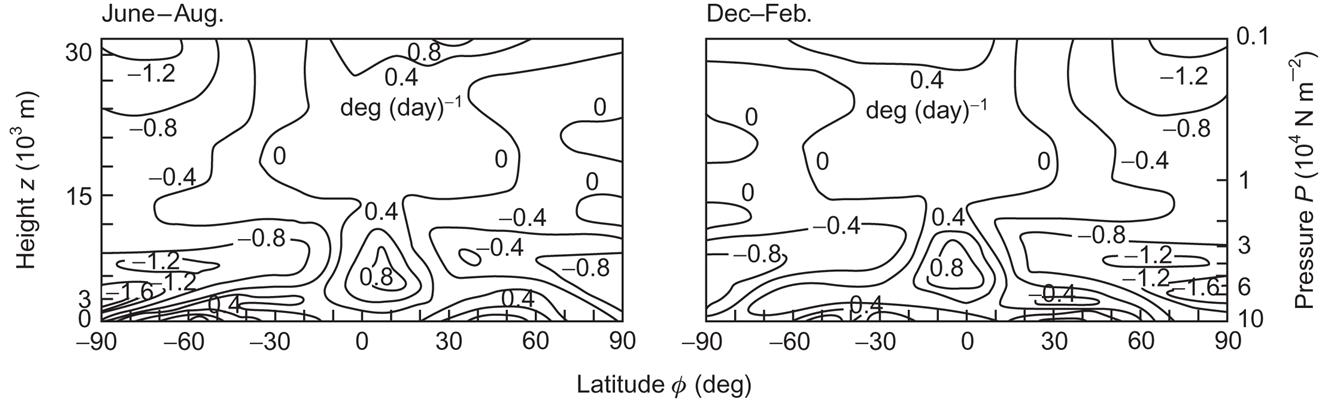
 , averaged over longitude and season (left: June–August, right: December–February). The unit is K (day)−1. Based on Newell et al. (1969).

The diabatic heating contributions integrated over a vertical column through the atmosphere are indicated in Fig. 2.108. The difference between radiation absorbed and re-emitted from the atmosphere, ![]() , is negative and fairly independent of latitude. The heat of condensation, which is approximated by the precipitation rate ra times the latent heat of vaporization Lv, varies substantially with latitude, depending primarily on the distribution of land and ocean surfaces. The heat added to the atmosphere by turbulent convection is equal to the net sensible heat flow at the Earth’s surface, with opposite sign, i.e.,
, is negative and fairly independent of latitude. The heat of condensation, which is approximated by the precipitation rate ra times the latent heat of vaporization Lv, varies substantially with latitude, depending primarily on the distribution of land and ocean surfaces. The heat added to the atmosphere by turbulent convection is equal to the net sensible heat flow at the Earth’s surface, with opposite sign, i.e., ![]() . The sum of the three contributions shown in Fig. 2.108 is not zero, but has to be supplemented by the transport of sensible heat in the atmosphere, between the different latitude areas. However, this is exactly what the equations of motion are supposed to describe.
. The sum of the three contributions shown in Fig. 2.108 is not zero, but has to be supplemented by the transport of sensible heat in the atmosphere, between the different latitude areas. However, this is exactly what the equations of motion are supposed to describe.

 is the net radiation flux, Lvra is the heat gained by condensation of water vapor, and
  is the turbulent flux of sensible heat from the Earth’s surface to the atmosphere (i.e., the same quantities appearing in Figs. 2.106 and 2.107, but integrated over height). The deviation of the sum of the three quantities from zero should equal the heat gain from horizontal transport of sensible heat
  . Based on Sellers (1965).
2.5.2.3 Separation of scales of motion
The averaging procedure discussed in conjunction with (2.23) presumes that a “large” and a “small” scale of motion are defined. This may be properly done by performing a Fourier analysis of the components of the wind velocity vector, or of the wind speed |v|. It is convenient to consider the variance of the wind speed (because it is proportional to a kinetic energy), defined by ![]() . The brackets
. The brackets ![]() denote average over a statistical ensemble, corresponding to a series of actual measurements. Writing the spectral decomposition in the form
denote average over a statistical ensemble, corresponding to a series of actual measurements. Writing the spectral decomposition in the form
one obtains a form-invariant spectral function S(ω), which is shown in Fig. 2.109, based on a modern version of a pioneering measurement effort made by Hoven (1957). The peaks exhibited by the spectrum vary in magnitude with the height of measurement (cf. Fig. 3.37).

A striking feature of the spectrum in Fig. 2.109 (and the analogues for other heights) is the broad gap between ω≈0.5 h−1 and ω≈20 h−1. A large number of measurements have confirmed that the existence of such a gap is an almost universal feature of the wind speed spectrum. Its significance is to provide a clear distinction between the region of large-scale motion (ω ![]() 0.5 h−1) and the region of small-scale (eddy) motion (ω
0.5 h−1) and the region of small-scale (eddy) motion (ω ![]() 5 h−1). The existence of the gap makes the time-averaging procedure in (2.21) easy and makes the exact choice of Δt insignificant over a reasonably large interval, so that the resulting large-scale motion is not critically dependent on the prescription for time averaging. One should be warned, however, not to conclude that the gap in Fig. 2.109 indicates that large-scale motion and small-scale motion are not coupled. It is not necessary for such couplings to involve all intermediate frequencies; on the contrary, distinct couplings may involve very different scales of motion in a straightforward way. Examples of this are evident in the equations of motion, such as (2.48), which allows kinetic energy to be taken out of the large-scale motion (V*) and be put into small-scale motion
5 h−1). The existence of the gap makes the time-averaging procedure in (2.21) easy and makes the exact choice of Δt insignificant over a reasonably large interval, so that the resulting large-scale motion is not critically dependent on the prescription for time averaging. One should be warned, however, not to conclude that the gap in Fig. 2.109 indicates that large-scale motion and small-scale motion are not coupled. It is not necessary for such couplings to involve all intermediate frequencies; on the contrary, distinct couplings may involve very different scales of motion in a straightforward way. Examples of this are evident in the equations of motion, such as (2.48), which allows kinetic energy to be taken out of the large-scale motion (V*) and be put into small-scale motion ![]() or vice versa.
or vice versa.
Thus small- and large-scale motions in the atmosphere are well-defined concepts, and no accurate model of the atmospheric circulation can be obtained without treating both simultaneously. Current modeling, both for short-term behavior of the atmospheric circulation (“weather forecasts”) and for long-term behavior (“climate change”), uses averaged values of terms coupling the scales and thus effectively only includes large-scale variables. This is the reason for the poor validity of weather forecasts: they remain valid only as long as the coupling terms involving turbulent (chaotic) motion do not change. For climate modeling, the constraints offered by the system boundaries make the model results valid in an average sense, but not necessarily the detailed geographical distribution of the magnitude of climate variables. This also means that the stability of the atmosphere, which as mentioned in section 2.4 is not in its lowest energy state, cannot be guaranteed by this type of calculation and that the atmosphere could experience transitions from one relatively stability state to another (as it has during its history, as evidenced by the transitions to ice ages and back).
Furthermore, since the motion within the atmosphere is not capable of carrying out all the necessary transport of heat (see Fig. 2.48), an accurate model of the circulation of the atmosphere is not possible without including the heat transport within the ocean–continent system (ocean currents, rivers, run-off along the surface, and, to a lesser extent, as far as heat transport is concerned, ground water motion). Such coupled models are considered below, after introducing the energy quantities of relevance for the discussion.
2.5.2.4 Energy conversion processes in the atmosphere
The kinetic energy of the atmospheric circulation can be diminished by friction, leading to an irreversible transformation of kinetic energy into internal energy (heat). In order to make up for frictional losses, new kinetic energy must be created in the atmosphere. This can be achieved by one of two processes, both of which are reversible and may proceed adiabatically. One is the conversion of potential energy into kinetic energy (by gravitational fall), and the other is the transformation of internal energy into kinetic energy by motion across a pressure gradient. In terms of the averaged quantities (i.e., neglecting terms like ![]() ), the kinetic, potential, and internal energies may be written
), the kinetic, potential, and internal energies may be written
(2.55)
 (2.55)
and the corresponding changes in time
(2.56)
obtained from (2.46) by scalar multiplication with v*,
(2.57)
[from the definition in (2.55)] and
(2.58)
which follows from (2.53) by using
and adding the heat gained by turbulent convection on the same footing as the external heat sources ρQ (radiation and gain of latent heat by condensation). As noted by Lorenz (1967), not all potential and internal energy is available for conversion into kinetic energy. The sum of potential and internal energy must be measured relative to a reference state of the atmosphere. Lorenz defines the reference state as a state in which the pressure equals the average value on the isentropic surface passing through the point considered [hence the convenience of introducing the potential temperature (2.52)].
2.5.2.5 Modeling the oceans
As mentioned in section 2.3, the state of the oceans is given by the temperature T, the density ρ=ρw (or alternatively the pressure P), the salinity S (salt fraction by mass), and possibly other variables, such as oxygen and organic materials present in the water. S is necessary in order to obtain a relation defining the density that can replace the ideal gas law used in the atmosphere. An example of such an equation of state, derived on an empirical basis by Eckart (1958), is
(2.59)
where x0 is a constant and x1 and x2 are polynomials of second order in T and first order in S*.
The measured temperature and salinity distributions are shown in Figs. 2.67–2.69. In some studies, the temperature is instead referred to surface pressure, thus being the potential temperature θ defined according to (2.52). By applying the first law of thermodynamics, (2.53), to an adiabatic process (Q=0), the system is carried from temperature T and pressure P to the surface pressure P0 and the corresponding temperature θ=T(P0). The more complex equation of state (2.59) must be used to express d(1/ρ) in (2.53) in terms of dT and dP,
where
This is then inserted into (2.53) with Q=0, and (2.53) is integrated from (T, P) to (θ, P0). Because of the minimal compressibility of water (as compared to air, for example), the difference between T and θ is small.
2.5.2.6 Basic equations governing the oceanic circulation
Considering first a situation where the formation of waves can be neglected, the wind stress may be used as a boundary condition for the equations of motion analogous to (2.47). The “Reynold stress” eddy transport term may, as mentioned in connection with (2.47), be parametrized as suggested by Boussinesq, so that it gets the same form as the molecular viscosity term and—more importantly—can be expressed in terms of the averaged variables,
(2.60)
Here use has been made of the anticipated insignificance of the vertical velocity, w*, relative to the horizontal velocity, V*. A discussion of the validity of the Boussinesq assumption may be found in Hinze (1975). It can be seen that (2.60) represents diffusion processes that result from introducing a stress tensor of the form (2.31) into the equations of motion (2.47). In (2.60), the diffusion coefficients have not been assumed to be isotropic, but in practice the horizontal diffusivities kx and ky are often taken to be equal (and denoted K; Bryan, 1969; Bryan and Cox, 1967). Denoting the vertical and horizontal velocity components in the ocean waters ww and Vw, the averaged equations of motion, corresponding to (2.48) and (2.49) for the atmosphere, become
(2.61)
where T should be inserted in °C (Bryan, 1969).
(2.62)
 (2.62)
where the Coriolis parameter is
in terms of the angular velocity of the Earth’s rotation, Ω, plus the longitudinal angular velocity of the mean circulation, ![]() (rs cos ϕ)−1, with rs being the radius of the Earth.
(rs cos ϕ)−1, with rs being the radius of the Earth.
The boundary conditions at the ocean’s surface are
(2.63)
 (2.63)
where τ is the wind stress (2.43). The boundary condition (2.63) [cf. (2.31)] reflects the intuitive notion that, for a small downward diffusion coefficient, kz, a non-zero wind stress will lead to a steep velocity gradient at the ocean surface. Knowledge of kz is limited, and in oceanic calculations kz is often taken as a constant, the value of which is around 10−4 m2 s−1 (Bryan, 1969).
If the density of water, ρw, is also regarded as a constant over time intervals much larger than that used in the averaging procedure, then the equation of continuity (2.46) simply becomes
(2.64)
Since the pressure, Pw in (2.61), is related to temperature and salinity through the equation of state, (2.59), a closed set of equations for the oceanic circulation must encompass transport equations analogous to (2.50) for the average values of temperature and salinity,
(2.65)
The turbulent diffusion coefficients, kz and K, being phenomenological quantities, could eventually be chosen separately for temperature, A*=Tw*, and salinity, A*=Sw*, and not necessarily be identical to those used in (2.62) for momentum. If it is assumed that there are no sources or sinks of heat or salt within the ocean, the right-hand side of (2.65) may be replaced by zero. The exchange of heat and salt between the ocean and the atmosphere can then be incorporated into the boundary conditions, under which the two equations (2.65) are solved,
(2.66)
(2.67)
Among the chemical reaction terms that have been suggested for inclusion as source terms, SA in (2.50), are the sulfate-forming reactions found in sea-salt spray particles (Laskin et al., 2003).
The surface net energy flux ![]() [cf. (2.18)], the evaporation e, and precipitation r are variables that link the ocean with the atmosphere, as well as the wind stress appearing in (2.63). In (2.66), Cw is the specific heat of water.
[cf. (2.18)], the evaporation e, and precipitation r are variables that link the ocean with the atmosphere, as well as the wind stress appearing in (2.63). In (2.66), Cw is the specific heat of water.
The above expressions do not include the contributions from ice-covered water. Bryan (1969) has constructed boundary conditions allowing for formation and melting of sea ice. Pack ice extending to a depth of less than 3 m is able to move, so Bryan adds a transport equation for such sea ice in the general form of (2.65) and with a suitable source term. More recent models include a specific ice cover model and take into account both melting and sublimation processes (see, for example, NCAR, 1997).
2.5.2.7 Recent model applications surveyed in the 4th and 5th IPCC assessment
For several years, climate models have continuously improved, both with respect to resolution (currently down to about 25 km for the spatial grids used, leading to some 125 km accuracy of the final calculation results) and with respect to effects included. Recent models treat sea ice formation and movements, as well as details of cloud cover and its influence on both water cycle and air properties. To be considered in the models are the coupling between glaciation, depression and upheaval of the crust, and the associated changed in sea shorelines (Peltier, 1994; 2004). These are not only important for reproducing past climates but also for understanding the effects of ice melting in Greenland and Antarctica. Therefore, modeling efforts are directed not only at future climates, but also as the past ones as they are relevant for a basic understanding of climate change, whether anthropologically induced or not (Kaspar and Cubasch, 2007; Jansen et al., 2007; NOAA, 2010; Sørensen, 2011).
The development since the 2007 publication of the 4th Assessment of the Intergovernmental Climate Panel IPCC has not significantly improved resolution, but has concentrated on improving those submodels that have failed to reproduce observed traits. The 5th Assessment Report (IPCC, 2013a,b) is a survey of ongoing work in this respect, still with many open ends. The original purpose of the IPCC was to evaluate published work related to climate change, but because the model improvements are becoming more marginal, scientific journals now only publish results containing a specific new insight, and the IPCC has therefore increasingly been basing its model assessment on commissioned computer runs from a selection of climate science centers. Much of the assessment in and after the 5th report has had the character of inter-comparison of this set of models, and many of the Figures in the 5th report show the significant spread of model results from different models. Because the models include different effects that might influence the global climate, in addition to the standard inclusion of the effect of greenhouse gases and other forcing components, the comparison could reveal which additional effects that are most important, but variance could also be ascribed to differences in the programming details (or even errors). In any case, the dependence of IPCC on the centers making these calculations may be the reason that little effort is directed at identifying the “best” models.
There are more fundamental problems in the way the IPCC is operating. The Working Group I responsible for modeling the physical aspects of the Earth’s climate needs input of emissions and other data that may influence the modeling. The two other working groups dealing with effects of climate change and mitigation or adaptation options depend on the output from the Working Group 1 climate models in order to perform their tasks, but such output is not forthcoming without knowing the input assumptions. These may to an extent draw on the reflections offered by the Working Groups 2 and 3, but to ease the process, IPCC has commissioned a set of emission scenarios from an outside group resembling the setup of the working groups but strongly leaning on the traditional energy industry, as evidenced by the scenarios created. Probably the reason for regarding the essential emission scenario input as external to the IPCC mission is historical, as the first IPCC Assessments just had to use the assumptions of available published climate model studies. For many years, these used just a doubling or quadrupling of greenhouse gas emissions relative to pre-industrial levels, without any deeper reflections on alternatives to the neo-liberal economic growth model that has shaped the energy behavior during the last three decades. Considering the many alternative economic approaches that have been in vogue earlier and are debated today (such as welfare, socialist or sustainable economies, cf. Sørensen, 2016), it would seem a very strong assumption to imbed projections by climate modeling aimed to extend centuries into the future into one possibly short-lived economic mantra.
The emission scenarios commissioned for the 4th Assessment (Nakićenović et al., 2000) are based on interview studies, in principle accepting input from anyone. In reality, NGOs and independent scientists submitted what they saw as the best scenarios for a sustainable future, while energy industry (and particularly electric utility companies in Japan) submitted business-as-usual scenarios, often with some 25 variants. Somebody must have told them that the submissions would be treated statistically. It is not helpful when Nakićenović et al. warns against using expressions like “business-as-usual” or “best” scenarios, when the selection procedure has disfavored anything involving new economic paradigms or premature phasing out of conventional energy resources before their price rises due to shortage of resources. As a result, the 2001 and 2007 IPCC scenarios became dominated by fossil growth scenarios, the 100% renewable scenarios in the scientific literature were treated as anomalies outside the statistical confidence limits, and the only scenarios with lower emissions included were described as a stagnation scenario with little economic development and extensive poverty due to decisions being made locally and a lack of globalization. The actual development has in several ways proven these assumptions incorrect. Zero-emission energy technologies are growing fast, energy efficiency improvement is in some sectors halting energy growth while maintaining economic revenues, and emissions of particulate matter is declining faster than assumed in the 4th Assessment.
As a consequence, IPCC has had to modify its emission scenarios for the 5th Assessment. They are now characterized by forcings (see Fig. 7.16 and accompanying text) ranging from 2.6 to 8.5 W m−2, leading to average global warming by year 2100 of 1.5−5.0°C (Moss et al., 2010; IPCC, 2013b). The scenarios are now recognizing increased energy efficiency but the most promising renewable energy resources (wind and solar) are hardly used, while bio-energy use is extensive in three of the scenarios. The high-forcing scenario assumes a 7–8 times increase in use of coal, relative to year 2000 (Vuuren et al., 2011). The apparently wide range of scenarios is clearly only a subset of possibilities, representing a very conventional outlook, and the low-emission IPCC scenario have implications for social development very different from those associated with the segments of current societies wishing to see a sustainable future based on renewable energy.
The examples of climate model output given in Figs. 2.110 and 2.111 for temperature and precipitation are taken from what is considered one of the best models of work underlying the 4th Assessment, not bothering with the small changes in some of the 5th Assessment runs. The Japanese model behind Fig. 2.110 has been run from the pre-industrial situation prevailing around 1860, and for various emission scenarios for future emissions of greenhouse gases. Figure 2.110 picks the A1B scenario, which is close to the “business-as-usual” scenario (IS92a; cf. Fig 2.101) of previous IPCC assessments. That scenario was an exponential growth scenario mainly based on fossil energy resources. The A1B scenario still assumes that the current 18th-century economic paradigm prevails but recognizes that in some parts of the world there is a discussion of limited resources and carrying capability of the environment. The emission scenario assumes that a mixture of fossil, nuclear, and renewable energy resources will be employed, as dictated by market prices without externalities during the unrestrained economic growth. Miraculously, world population stabilizes and the CO2 concentration in the atmosphere stabilizes at 720 ppm toward the end of the 21st century (causes invoked may be the decline in fertility characterizing presently rich countries to spread, but this is a controversial issue related to the outlook for reducing economic inequality, inside and between countries, where currently disparity between rich and poor seem to rise everywhere; Sørensen, 2016).


Compared to the earlier model results shown in Fig. 2.101, for a doubling of CO2 but relative to about 1995, the new 2055 numbers, expected to represent a comparable situation, show increased warming, and in contrast to the 2020 results and the old 2055 values of Fig 2.101, there are now no regions with a lowering of temperature. Considering the different year of departure, the results can be considered consistent. These remarks are valid for both the January and the July results.
By 2090, warming is very strong, up to 25°C at the poles, and over 5°C when averaged over land areas. This is the expected outcome of the lack of political action characterizing the A1B emission scenario. The warming is predicted to affect high-latitude Northern areas already in 2020, by 2055 most areas in the northern United States, Siberia, and China. Mountain areas like the Himalayas experience strong warming, and both they and the arctic areas are likely to lose large amounts of ice. By 2090, all inhabited parts of the world are strongly affected, including South America, Africa, and Australia, and in both January and July.
The calculated effect of climate change on precipitation, shown in Fig. 2.111, shows a much stronger change than in temperature from pre-industrial times to the 2011–2030 period, and somewhat less during the rest of the 21st century, except for a pronounced reduction in the Eastern Equatorial Pacific and an even stronger increase in the Western Equatorial Pacific. A similar but more divided effect is seen in the Indian and Atlantic Oceans. This behavior is even stronger in July than in January. Generally, the dry areas in the northern half of Africa and in the Middle East become even dryer, and the high-latitude areas more wet. The U.S. Midwest is becoming dryer during July but is neutral in January, which could have implications for agriculture there, which is already considerably dependent on artificial irrigation. The opposite is the case for India, getting more summer rain in the southeast and considerably less in the northwest, including the already dry Rajasthan desert.
There is no conservation of the water cycle through the atmosphere: The amount of water evaporated from land and sea surfaces and later falling as precipitation increases, as one would expect due to the general warming.
The studies assessed by the (presently five) IPCC Working Group I reports have had a considerable effect on making decision-makers aware of the climate change problem associated with anthropogenic emissions. The success is largely due to the scientific credibility of the assessments, which was ensured when IPCC was formed, by following the suggestion by its first chairman, Bert Bolin, to deviate from the usual United Nations procedure of having governments designate members of committees (occasionally leading to the nomination of family members of say African leaders to committees that they had no expertise to be on, or to the nomination of energy–industry lobbyists). This was facilitated by not having IPCC subsumed under one UN agency, but sitting between two. When UN in 1997 after political pressure from climate change skeptic nations chose to revert working group member selection to traditional UN rules, Bolin resigned and the altered role of IPCC blurring the division between scientific assessment and political recommendations has therefore been questioned (Hulme et al., 2010). Governments may nominate good scientists to the IPCC working groups, but they may also nominate some that can advance a particular government’s attitude toward acting on the warming threat. The main message in the IPCC report has, however, remained unchanged and attacks from various lobby groups have so far not been able to shake its substance. After all, the greenhouse effect is an established physical fact and although many additional effects that add to the behavior of climate are important, they largely serve to qualify the indisputable main effects. Those (e.g., some sunspot scientists) who think that finding new effects will automatically invalidate classical physics are clearly at variance with scientific rationality. The situation for the two other working groups is different and will be dealt with in Chapter 7.
2.5.3 Tides and Waves
Consider a celestial body of mass M and distance R from the center of the Earth. The gravitational force acting on a particle of mass m placed at distance r from the Earth’s center may, in a co-ordinate system moving with the Earth, be written
where R′ is the position vector of the mass m relative to M. The force may be decomposed into a radial and a tangential part (along unit vectors er and et), introducing the angle θ between −R and r and assuming that |r| is much smaller than |R| and |R′| in order to retain only the first terms in an expansion of R′−2 around R−2,
(2.68)
If the particle m is at rest within or near to the Earth, it is further influenced by the gravitational force of the mass of the sphere inside its radius, with the center coinciding with that of the Earth. If the particle is following the rotation of the Earth, it is further subjected to the centrifugal force and, if it is moving relative to the Earth, to the Coriolis force. The particle may be ascribed a tidal potential energy, taken to be zero if the particle is situated at the center of the Earth (Bartels, 1957),
If the particle is suspended at the Earth’s surface in such a way that it may adjust its height, so that the change in its gravitational potential, mgz, can balance the tidal potential, then the change in height, z=Δr, becomes
If one inserts lunar mass and mean distance, this height becomes z=0.36 m for cos2θ=0, i.e., at the points on the Earth facing the Moon or opposite (locations where the Moon is in zenith or in nadir). Inserting instead data for the Sun, the maximum z becomes 0.16 m. These figures are equilibrium tides that might be attained if the Earth’s surface were covered with ocean and if other forces, such as those associated with the Earth’s rotation, were neglected. However, since water would have to flow into the regions near θ=0 and θ=π, and since water is hardly compressible, volume conservation would require lowering of the water level at θ=π/2.
The estimate of “equilibrium tides” only serves the purpose of a zero-order orientation of the magnitude of tidal effects originating from different celestial bodies. The actual formation of tidal waves is a dynamic process that depends not only on the above-mentioned forces acting on the water particles, but also particularly on the topography of the ocean boundaries. The periods involved can be estimated by inserting into (2.68) the expression for the zenith angle θ of the tide-producing celestial body, in terms of declination δ and hour angle ω of the body,
[cf. the discussion in connection with (2.9) and (2.10)]. The tidal force will have components involving cosω and cos2ω=(cos(2ω)+1)/2, or the corresponding sine functions, which proves the existence of periods for lunar tides equal to one lunar day (24 h and 50 min) and to half a lunar day. Similarly, the solar tides are periodic with components of periods of a half and one solar day. If higher-order terms had been retained in (2.68), periods of a third the basic ones, etc., would also be found, but with amplitudes only a small fraction of those considered here.
Owing to the inclination of the lunar orbital plane relative to that of the Earth–Sun system, the amplitudes of the main solar and lunar tidal forces (2.68) will add in a fully coherent way only every 1600 years (latest in 1433; Tomaschek, 1957). However, in case of incomplete coherence, one can still distinguish between situations where the solar tidal force enhances that of the Moon (“spring tide”) and situations where the solar tidal forces diminish the lunar tides (“neap tide”).
Tidal waves lose energy due to friction against the continents, particularly at inlets with enhanced tidal changes in water level. It is estimated that this energy dissipation is consistent with being considered the main cause for the observed deceleration in the Earth’s rotation (the relative decrease being 1.16×10⁻¹⁰ per year). Taking this figure to represent the energy input into tidal motion, as well as the frictional loss, one obtains a measure of the energy flux involved in the tides as equal to about 3×10¹² W (King Hubbert, 1969).
2.5.3.1 Gravity waves in the oceans
The surface of a wavy ocean may be described by a function σ=σ(x, y, t), giving the deviation of the vertical co-ordinate z from zero. Performing a spectral decomposition of a wave propagating along the x-axis yields
(2.69)
where S(k) represents the spectrum of σ. If ω is constant and positive, (2.69) describes a harmonic wave moving toward the right; if ω is constant and negative, the wave moves toward the left. By superimposing waves with positive and negative ω, but with the same spectral amplitude S(k), standing waves may be constructed. If S(k) in (2.69) is different from zero only in a narrow region of k-space, σ will describe the propagation of a disturbance (wave packet) along the ocean surface.
The wave motion should be found as a solution to the general equations of motion (2.61)–(2.64), removing the time averages and interpreting the eddy diffusion terms as molecular diffusion (viscous) terms, with the corresponding changes in the numerical values of kx=K into ηw (the kinematic viscosity of water, being around 1.8×10⁻⁶ m2 s−1). Owing to the incompressibility assumption (2.64), the equation of motion in the presence of gravity as the only external force may be written
(2.70)
For irrotational flow, rot ν=0, the velocity vector may be expressed in terms of a velocity potential, ϕ (x, y, z, t),
(2.71)
and the following integral to the equation of motion exists,
(2.72)
where the constant on the right-hand side is only zero if proper use has been made of the freedom in choosing among the possible solutions ϕ to (2.71). In the case of viscous flow, rot vw is no longer zero, and (2.71) should be replaced by
(2.73)
A lowest-order solution to these equations may be found using the infinitesimal wave approximation (Wehausen and Laitone, 1960) obtained by linearizing the equations [i.e., disregarding terms like ![]() in (2.72), etc.]. If the surface tension, which would otherwise appear in the boundary conditions at z=0, is neglected, one obtains the first-order, harmonic solution for gravity waves, propagating in the x-direction,
in (2.72), etc.]. If the surface tension, which would otherwise appear in the boundary conditions at z=0, is neglected, one obtains the first-order, harmonic solution for gravity waves, propagating in the x-direction,
(2.74)
(2.75)
where the connection between wave velocity (phase velocity) Uw, wave number k, and wavelength λw is
(2.76)
[cf. the relation in the presence of surface tension (2.27)]. No boundary condition has been imposed at the bottom, corresponding to a deep ocean assumption, λw![]() h, with h being the depth of the ocean. If the viscous forces are disregarded, the lowest-order solutions are similar to those of (2.74) and (2.75), but with the last exponential factor omitted. Improved solutions can be obtained by including higher-order terms in the equations of motion, by perturbative iteration starting from the first-order solutions given here. The second-order correction to ϕ is zero, but the wave surface (2.75) becomes (for ηw≈0)
h, with h being the depth of the ocean. If the viscous forces are disregarded, the lowest-order solutions are similar to those of (2.74) and (2.75), but with the last exponential factor omitted. Improved solutions can be obtained by including higher-order terms in the equations of motion, by perturbative iteration starting from the first-order solutions given here. The second-order correction to ϕ is zero, but the wave surface (2.75) becomes (for ηw≈0)
The correction makes the wave profile flatter along the bottom (trough) and steeper near the top (crest). Exact solutions to the wave equations, including surface tension but neglecting viscous forces, have been constructed (see, for example, Havelock, 1919). An important feature of these solutions is a maximum value that the ratio between wave amplitude a and wavelength λw can attain, the numerical value of which is determined as
(2.77)
As already suggested by Stokes (1880), the “corner” occurring at the crest of such a wave would have an angle of 120°. Figure 2.112 indicates the form of the gravity wave of maximum amplitude-to-wavelength ratio. For capillary waves, the profile has opposite characteristics: the crest is flattened, and a corner tends to develop in the trough.

2.5.3.2 The formation and dissipation of energy in wave motion
The energy of wave motion is the sum of potential, kinetic, and surface contributions (if surface tension is considered). For a vertical column of unit area, one has
(2.78)
(2.79)
 (2.79)
(2.80)
Thus, for the harmonic wave (2.74) and (2.75), the total energy, averaged over a period in position x, but for a fixed time t, and neglecting ![]() , is
, is
(2.81)
This shows that a wave that does not receive renewed energy input will dissipate energy by molecular friction, with the rate of dissipation
(2.82)
Of course, this is not the only mechanism by which waves lose energy. Energy is also lost by the creation of turbulence on a scale above the molecular level. This may involve interaction with the air, possibly enhanced by the breaking of wave crests, or oceanic interactions due to the Reynold stresses (2.60). Also, at the shore, surf formation and sand put into motion play a role in energy dissipation from wave motion.
Once the wind has created a wave field, it may continue to exist for a while, even if the wind ceases. If only frictional dissipation of the type (2.82) is active, a wave of wavelength λw=10 m will take 70 h to be reduced to half the original amplitude, while the time is 100 times smaller for λw=1 m.
The detailed mechanisms by which a wave field is created by the wind field, and subsequently transfers its energy to other degrees of freedom, are not understood in detail. According to Pond (1971), about 80% of the momentum transfer from the wind may be going initially into wave formation, implying that only 20% goes directly into forming currents. Eventually, some of the energy in wave motion is transferred to the currents.
2.5.3.3 The energy flux associated with wave motion
Now reconsider a single, spectral component of the wave field. The energy flux through a plane perpendicular to the direction of wave propagation, i.e., the power carried by the wave motion, is given in the linearized approximation by (Wehausen and Laitone, 1960)
(2.83)
For the harmonic wave (2.74) and (2.75), neglecting surface tension, this gives
(2.84)
when averaged over a period. Since (g/k)1/2=Uw, this together with (2.81) for ηw=0 gives the relationship
(2.85)
Thus the energy is not transported by the phase velocity Uw, but by 1/2Uw. For a spectral distribution, the power takes the form
(2.86)
where Ug(k) is the group velocity d(kUw)/dk (equal to 1/2Uw for the ocean gravity waves considered above). It is no surprise that energy is transported by the group velocity, but (2.85) and (2.84) show that this is the case even if there is no group (or wave packet) at all, i.e., for a single, sinusoidal wave.
2.5.3.4 Wind-driven oceanic circulation
The generation of currents by a part of the wind stress, or maybe as an alternative dissipation process for waves (Stewart, 1969), can be described by the equation of motion (2.62), with the boundary condition (2.63) eventually reducing τ by the amount spent in the formation of waves. Considering the Coriolis and vertical friction terms as the most important ones, Ekman (1902) writes the solution in the form
where z is the directional angle of the surface stress vector (measured from the direction of the x-axis) and
(f is the Coriolis parameter). The surface velocity vector is directed 45° to the right of the stress vector, and it spirals down with decreasing length. The average mass transport is perpendicular to the wind stress direction, 90° to the right. The observed angle at z≈0 is about 10° rather than 45° (Stewart, 1969), supporting the view that more complicated processes take place in the surface region. The gross mass transport, however, is well established, for example, in the North Atlantic Ocean, where water flows into the Sargasso Sea both from the south (driven by the prevailing eastward winds at the Equator) and from the north (driven by the mid-latitude “westerlies”).
In the Sargasso Sea, the assembled water masses are pressed downward and escape to the sides at a depth. All the water masses are, on average, following the rotation of the Earth, but the lateral squeezing process causes a change in rotational speed of the water involved, in particular a reduction in the vertical component of the angular speed vector. If the rotational speed of some mass of water does not fit with the rotation of the solid Earth at the latitude in question, the water mass will try to move to another latitude that is consistent with its angular speed (unless continents prevent it from doing so). For this reason, the water masses squeezed out below the Sargasso Sea move toward the Equator. Later, they have to return northward (otherwise, the polar part of the Atlantic Ocean would be emptied). Also, in this case, the rotation has to be adjusted to conserve angular momentum. This change in rotation is achieved by frictional interaction with the western continents. Owing to the sense of the Earth’s rotation, these return flows (e.g., the Gulf Stream) have to follow western shores, whether the return flow is northward or southward.
A description is provided above of how the wind drives the Ekman flow in the Atlantic Ocean, which induces its major currents. Similar mechanisms are present in the other oceans. Models of these flows, as well as the flows generated by sinking cold water (i.e., not by the winds), have been constructed and integrated along with the atmospheric models considered in section 2.3.1 (Manabe, 1969; Bryan, 1969; Wetherald and Manabe, 1972).