
The energy conversion processes
Abstract
This chapter contains the engineering basis for renewable energy conversion into desired energy supply forms. After introducing the general transformation theory for mechanical and thermodynamic processes, the treatment of specific heat and electricity conversion systems are described. Engines, heat pumps, boilers, furnaces, a range of flow-driven converters, photovoltaic and photothermal devices, coolers, electrochemical converters such as fuel cells, and tools for biological conversion into heat or power.
Keywords
Thermodynamic engine cycles; Thermoelectric conversion; Heat pumps; Wind energy converters; Hydro energy; Wave energy converters; Photovoltaic cells; Solar thermal panels; Combines solar power and heat modules; Combustion; Biological conversion of energy; Enzymatic decomposition
4.1 General principles
A large number of energy conversion processes take place in nature, some of which are described in Chapters 2 and 3. Mankind is capable of performing additional energy conversion processes by means of various devices invented. Such devices may be classified according to the type of construction used, according to the underlying physical or chemical principle, or according to the forms of energy appearing before and after the action of the device. This chapter surveys methods that may be suitable for the conversion of renewable energy flows or stored energy. A discussion of general conversion principles is made below, followed by an outline of engineering design details for specific energy conversion devices, ordered according to the energy form being converted and the energy form obtained. The collection is necessarily incomplete and involves judgment about the importance of various devices.
4.1.1 Basic principles of energy conversion
Table 4.1 lists some examples of energy conversion processes or devices currently in use or contemplated, organized according to the energy form emerging after the conversion. In several cases, more than one energy form emerges as a result of the action of the device; for example, heat in addition to one of the other energy forms listed. Many devices also perform several energy conversion steps, rather than the single ones given in the table. A power plant, for example, may perform the conversion process chain between the energy forms: chemical→heat→mechanical→electrical. Diagonal transformations are also possible, such as conversion of mechanical energy into mechanical energy (potential energy of elevated fluid→kinetic energy of flowing fluid→rotational energy of turbine) or of heat into heat at a lower temperature (convection, conduction). A process in which the only change is heat transfer from a lower to a higher temperature is forbidden by the second law of thermodynamics. Such transfer can be established if at the same time some high-quality energy is degraded, for example, by a heat pump (which is listed as a converter of electrical into heat energy in Table 4.1, but is further discussed in section 4.2.3).
Table 4.1
Examples of energy conversion processes listed according to the initial energy form and one particular converted energy form (the one primarily wanted)
| Initial Energy Form | Converted Energy Form | ||||
| Chemical | Radiant | Electrical | Mechanical | Heat | |
| Nuclear | Reactor | ||||
| Chemical | Fuel cell, battery discharge | Burner, boiler | |||
| Radiant | Photolysis | Photovoltaic cell | Absorber | ||
| Electrical | Electrolysis, battery charging | Lamp, laser | Electric motor | Resistance, heat pump | |
| Mechanical | Electric generator, MHD | Turbines | Friction, churning | ||
| Heat | Thermionic & thermoelectric generators | Thermodynamic engines | Convector, radiator, heat pipe | ||

The efficiency with which a given conversion process can be carried out, that is, the ratio between the output of the desired energy form and the energy input, depends on the physical and chemical laws governing the process. For heat engines, which convert heat into work or vice versa, the description of thermodynamic theory may be used in order to avoid a complicated description on the molecular level (which is, of course, possible, for example, on the basis of statistical assumptions). According to thermodynamic theory (again, the second law), no heat engine can have an efficiency higher than that of a reversible Carnot process, which is depicted in Fig. 4.1, in terms of different sets of thermodynamic state variables,
and

Entropy is defined in (1.1), apart from an arbitrary constant fixed by the third law of thermodynamics (Nernst’s law), which states that S can be taken as zero at zero absolute temperature (T=0). Enthalpy H is defined by
(4.1)
in terms of P, V, and the internal energy U of the system. According to the first law of thermodynamics, U is a state variable given by
(4.2)
in terms of the amounts of heat and work added to the system [Q and W are not state variables, and the individual integrals in (4.2) depend on the paths of integration]. Equation (4.2) determines U up to an arbitrary constant, the zero point of the energy scale. Using definition (1.1),
and
both of which are valid only for reversible processes. The following relations are found among the differentials:
(4.3)
These relations are often assumed to have general validity.
If chemical reactions occur in the system, additional terms μi dni should be added on the right-hand side of both relations (4.3), in terms of the chemical potentials, which are discussed briefly in section 3.5.3.
For a cyclic process like the one shown in Fig. 4.1, ∫dU=0 upon returning to the initial locus in one of the diagrams, and thus, according to (4.3), ∫T dS=∫P dV. This means that the area enclosed by the path of the cyclic process in either the (P, V)- or the (T, S)-diagram equals the work −W performed by the system during one cycle (in the direction of increasing numbers in Fig. 4.1).
The amount of heat added to the system during the isothermal process 2-3 is ΔQ23=T(S3−S2), if the constant temperature is denoted T. The heat added in the other isothermal process, 4-1, at a temperature Tref, is ΔQ41=−Tref (S3−S2). It follows from the (T, S)-diagram that ΔQ23+ΔQ41=−W.
The efficiency by which the Carnot process converts heat available at temperature T into work, when a reference temperature of Tref is available, is then
(4.4)
The Carnot cycle (Fig. 4.1) consists of four steps: 1-2, adiabatic compression (no heat exchange with the surroundings, i.e., dQ=0 and dS=0); 2-3, heat drawn reversibly from the surroundings at constant temperature (the amount of heat transfer ΔQ23 is given by the area enclosed by the path 2-3-5-6-2 in the (T, S)-diagram); 3-4, adiabatic expansion; and 4-1, heat given away to the surroundings by a reversible process at constant temperature [|ΔQ41| is equal to the area of the path 4-5-6-1-4 in the (T, S)-diagram].
The (H, S)-diagram is an example of a representation in which energy differences can be read directly on the ordinate, rather than being represented by an area.
Long periods of time are required to perform the steps involved in the Carnot cycle in a way that approaches reversibility. Because time is important for human enterprises (the goal of the energy conversion process being power, rather than just an amount of energy), irreversible processes are deliberately introduced into the thermodynamic cycles of actual conversion devices. The thermodynamics of irreversible processes are described below using a practical approximation, which is referred to in several of the examples to follow. Readers without specific interest in the thermodynamic description may go lightly over the formulae.
4.1.1.1 Irreversible thermodynamics
The degree of irreversibility is measured in terms of the rate of energy dissipation,
(4.5)
where dS/dt is the entropy production of the system while it is held at the constant temperature T (i.e., T may be thought of as the temperature of a large heat reservoir, with which the system is in contact). In order to describe the nature of the dissipation process, the concept of free energy is introduced (cf. Prigogine, 1968; Callen, 1960).
The free energy, G, of a system is defined as the maximum work that can be drawn from the system under conditions where the exchange of work is the only interaction between the system and its surroundings. A system of this kind is said to be in thermodynamic equilibrium if its free energy is zero.
Consider now a system divided into two subsystems, a small one with extensive variables (i.e., variables proportional to the size of the system) U, S, V, etc., and a large one with intensive variables Tref, Pref, etc., which is initially in thermodynamic equilibrium. The terms small system and large system are meant to imply that the intensive variables of the large system (but not its extensive variables Uref, Sref, etc.) can be regarded as constant, regardless of the processes by which the entire system approaches equilibrium.
This implies that the intensive variables of the small system, which may not even be defined during the process, approach those of the large system when the combined system approaches equilibrium. The free energy, or maximum work, is found by considering a reversible process between the initial state and the equilibrium. It equals the difference between the initial internal energy, Uinit=U+Uref, and the final internal energy, Ueq, or it may be written (all in terms of initial state variables) as
(4.6)
plus terms of the form Σμi,refni if chemical reactions are involved, and similar generalizations in case of electromagnetic interactions, etc.
If the entire system is closed, it develops spontaneously toward equilibrium through internal, irreversible processes, with a rate of free energy change
assuming that the entropy is the only variable. S(t) is the entropy at time t of the entire system, and Ueq(t) is the internal energy that would be possessed by a hypothetical equilibrium state defined by the actual state variables at time t, i.e., S(t), etc. For any of these equilibrium states, ∂Ueq(t)/∂S(t) equals Tref according to (4.3), and by comparison with (4.5) it is seen that the rate of dissipation can be identified with the loss of free energy, as well as with the increase in entropy,
(4.7)
For systems met in practice, there are often constraints preventing the system from reaching the absolute equilibrium state of zero free energy. For instance, the small system considered above may be separated from the large one by walls that keep the volume V constant. In such cases, the available free energy (i.e., the maximum amount of useful work that can be extracted) becomes the absolute amount of free energy, (4.6), minus the free energy of the relative equilibrium that the combined system can be made to approach in the presence of the constraint. If the extensive variables in the constrained equilibrium state are denoted U0, S0, V0, etc., then the available free energy becomes
(4.8)
eventually with the additions involving chemical potentials, etc. In (4.6) or (4.8), G is called the Gibbs potential. If the small system is constrained by walls, so that the volume cannot be changed, the free energy reduces to the Helmholtz potential U−TS, and if the small system is constrained so that it is incapable of exchanging heat, the free energy reduces to the enthalpy (4.1).
The corresponding forms of (4.8) give the maximum work that can be obtained from a thermodynamic system with the given constraints.
A description of the course of an actual process as a function of time requires knowledge of equations of motion for the extensive variables, i.e., equations that relate the currents, such as
(4.9)
 (4.9)
(4.9)
to the (generalized) forces of the system. As a first approximation, the relation between the currents and the forces may be taken as linear (Onsager, 1931),
(4.10)
The direction of each flow component is Ji/Ji. The arbitrariness in choosing the generalized forces is reduced by requiring, as did Onsager, that the dissipation be given by
(4.11)
Examples of the linear relationships (4.10) are Ohm’s law, stating that the electric current Jq is proportional to the gradient of the electric potential (Fq α grad ϕ), and Fourier’s law (3.34) for heat conduction or diffusion, stating that the heat flow rate Esens=JQ is proportional to the gradient of the temperature.
Considering the isothermal expansion process required in the Carnot cycle (Fig. 4.1), heat must be flowing to the system at a rate JQ=dQ/dt, with JQ=LFQ according to (4.10) in its simplest form. Using (4.11), the energy dissipation takes the form
For a finite time Δt, the entropy increase becomes
so that in order to transfer a finite amount of heat ΔQ, the product ΔS Δt must equal the quantity (LT)−1 (ΔQ)2. For the process to approach reversibility, as the ideal Carnot cycle should, ΔS must approach zero, which is seen to imply that Δt approaches infinity. This qualifies the statement made in the beginning of this subsection that, in order to go through a thermodynamic engine cycle in a finite time, one has to give up reversibility and accept a finite amount of energy dissipation and an efficiency that is smaller than the ideal (4.4).
4.1.1.2 Efficiency of an energy conversion device
A schematic picture of an energy conversion device is shown in Fig. 4.2, and it is sufficiently general to cover most types of converters in practical use (Angrist, 1976; Osterle, 1964). There is a mass flow into the device and another one out from it, as well as incoming and outgoing heat flow. The work output may be in the form of electric or rotating shaft power.
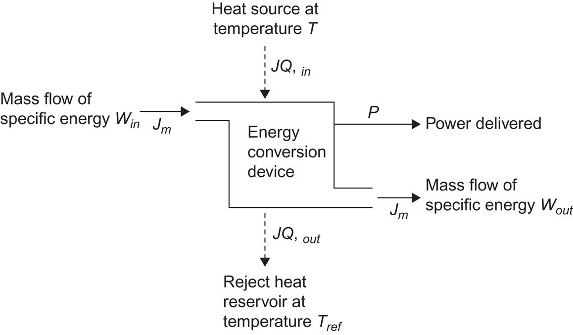
It may be assumed that the converter is in a steady state, implying that the incoming and outgoing mass flows are identical and that the entropy of the device itself is constant, i.e., that all entropy created is being carried away by the outgoing flows.
From the first law of thermodynamics, the power extracted, E, equals the net energy input,
(4.12)
The magnitude of the currents is given by (4.9), and their conventional signs may be inferred from Fig. 4.2. The specific energy content of the incoming mass flow, win, and of the outgoing mass flow, wout, are the sums of potential energy, kinetic energy, and enthalpy. The significance of the enthalpy to represent the thermodynamic energy of a stationary flow is established by Bernoulli’s theorem (Pippard, 1966). It states that for a stationary flow, if heat conduction can be neglected, the enthalpy is constant along a streamline. For the uniform mass flows assumed for the device in Fig. 4.2, the specific enthalpy, h, thus becomes a property of the flow, in analogy with the kinetic energy of motion and, for example, the geopotential energy,
(4.13)
The power output may be written
(4.14)
with the magnitude of currents given by (4.9) and the generalized forces given by
(4.15)
 (4.15)
corresponding to a mechanical torque and an electric potential gradient. The rate of entropy creation, i.e., the rate of entropy increase in the surroundings of the conversion device (as mentioned, the entropy inside the device is constant in the steady-state model), is
where sm,in is the specific entropy of the mass (fluid, gas, etc.) flowing into the device, and sm,out is the specific entropy of the outgoing mass flow. JQ,out may be eliminated by use of (4.12), and the rate of dissipation obtained from (4.7),
(4.16)
The maximum possible work (obtained for dS/dt=0) is seen to consist of a Carnot term (closed cycle, i.e., no external flows) plus a term proportional to the mass flow. The dissipation (4.16) is brought in the Onsager form (4.11),
(4.17)
by defining generalized forces
(4.18)
in addition to those of (4.15).
The efficiency with which the heat and mass flow into the device is converted to power is, in analogy to (4.4),
(4.19)
where expression (4.16) may be inserted for E. This efficiency is sometimes referred to as the “first law efficiency,” because it only deals with the amounts of energy input and output in the desired form and not with the “quality” of the energy input related to that of the energy output.
In order to include reference to the energy quality, in the sense of the second law of thermodynamics, account must be taken of the changes in entropy taking place in connection with the heat and mass flows through the conversion device. This is accomplished by the second law efficiency, which for power-generating devices is defined by
(4.20)
where the second expression is valid specifically for the device considered in Fig. 4.2, while the first expression is of general applicability, when max(E) is taken as the maximum rate of work extraction permitted by the second law of thermodynamics. It should be noted that max(E) depends not only on the system and the controlled energy inputs, but also on the state of the surroundings.
Conversion devices for which the desired energy form is not work may be treated in a way analogous to the example in Fig. 4.2. In (4.17), no distinction is made between input and output of the different energy forms. Taking, for example, electrical power as input (sign change), output may be obtained in the form of heat or in the form of a mass stream. The efficiency expressions (4.19) and (4.20) must be altered, placing the actual input terms in the denominator and the actual output terms in the numerator. If the desired output energy form is denoted W, the second law efficiency can be written in the general form
(4.21)
For conversion processes based on other principles than those considered in the thermodynamic description of phenomena, alternative efficiencies could be defined by (4.21), with max(W) calculated under consideration of the non-thermodynamic types of constraints. In such cases, the name “second law efficiency” would have to be modified.
4.1.2 Thermodynamic engine cycles
A number of thermodynamic cycles, i.e., (closed) paths in a representation of conjugate variables, have been demonstrated in practice. They offer examples of the compromises made in modifying the “prototype” Carnot cycle into a cycle that can be traversed in a finite amount of time. Each cycle can be used to convert heat into work, but in traditional uses the source of heat has mostly been the combustion of fuels, i.e., an initial energy conversion process, by which high-grade chemical energy is degraded to heat at a certain temperature, associated with a certain entropy production.
Figure 4.3 shows a number of engine cycles in (P, V)-, (T, S)-, and (H, S)- diagrams corresponding to Fig. 4.1.

The working substance of the Brayton cycle is a gas, which is adiabatically compressed in step 1-2 and expanded in step 3-4. The remaining two steps take place at constant pressure (isobars), and heat is added in step 2-3. The useful work is extracted during the adiabatic expansion 3-4, and the simple efficiency is thus equal to the enthalpy difference H3−H4 divided by the total input H3−H1. Examples of devices operating on the Brayton cycle are gas turbines and jet engines. In these cases, the cycle is usually not closed, since the gas is exhausted at point 4 and step 4-1 is thus absent. The somewhat contradictory name given to such processes is open cycles.
The Otto cycle, traditionally used in automobile engines, differs from the Brayton cycle in that steps 2-3 and 4-1 (if the cycle is closed) are carried out at constant volume (isochores) rather than at constant pressure.
The Diesel cycle (used in ship and truck engines, and, with the invention of the common-rail design, increasingly in passenger vehicles) has step 2-3 as isobar and step 4-1 as isochore, while the two remaining steps are approximately adiabatic. The actual design of conventional diesel engines may be found in engineering textbooks (e.g., Hütte, 1954), and new designs, such as the common-rail concept, are discussed in Sørensen (2006, 2010).
Closer to the Carnot ideal is the Stirling cycle, involving two isochores (1-2 and 3-4) and two isotherms.
The Ericsson cycle has been developed with the purpose of using hot air as the working fluid. It consists of two isochores (2-3 and 4-1) and two curves between isotherms and adiabates (cf., for example, Meinel and Meinel, 1976).
The last cycle is the one used in thermal power plants, the Rankine cycle depicted in Fig. 4.3. It has a more complicated appearance owing to the presence of two phases of the working fluid. Step 1-2-3 describes the heating of the fluid to its boiling point. Step 3-4 corresponds to the evaporation of the fluid, with both fluid and gaseous phases being present. It is an isotherm as well as an isobar. Step 4-5 represents the superheating of the gas, followed by an adiabatic expansion step 5-7. These two steps are sometimes repeated one or more times, with the superheating taking place at gradually lowered pressure, after each step of expansion to saturation. Finally, step 7-1 again involves mixed phases with condensation at constant pressure and temperature. The condensation often does not start until a temperature below that of saturation is reached. Useful work is extracted during the expansion step 5-7, so the simple efficiency equals the enthalpy difference H5−H7 divided by the total input H6−H1. The second law efficiency is obtained by dividing the simple efficiency by the Carnot value (4.4), for T=T5 and Tref=T7.
Thermodynamic cycles like those in Figs. 4.1 and 4.3 may be traversed in the opposite direction, thus using the work input to create a low temperature Tref (cooling, refrigeration; T being the temperature of the surroundings) or to create a temperature T higher than that (Tref) of the surroundings (heat pumping). In this case, step 7-5 of the Rankine cycle is a compression (8-6-5 if the gas experiences superheating). After cooling (5-4), the gas condenses at the constant temperature T (4-3), and the fluid is expanded, often by passage through a nozzle. The passage through the nozzle is considered to take place at constant enthalpy (2-9), but this step may be preceded by undercooling (3-2). Finally, step 9-8 (or 9-7) corresponds to evaporation at the constant temperature Tref.
For a cooling device, the simple efficiency is the ratio of the heat removed from the surroundings, H7−H9, and the work input, H5−H7, whereas for a heat pump it is the ratio of the heat delivered, H5−H2, and the work input. Such efficiencies are often called coefficients of performance (COP), and the second law efficiency may be found by dividing the COP by the corresponding quantity εCarnot for the ideal Carnot cycle (cf. Fig. 4.1),
(4.22a)
(4.22b)
In practice, the compression work H5−H7 (for the Rankine cycle in Fig. 4.3) may be less than the energy input to the compressor, thus further reducing the COP and the second law efficiency, relative to the primary source of high-quality energy.
4.2 Heat energy conversion processes
4.2.1 Direct thermoelectric conversion
If the high-quality energy form desired is electricity, and the initial energy is in the form of heat, there is a possibility of utilizing direct conversion processes, rather than first using a thermodynamic engine to create mechanical work followed by a second conversion step using an electricity generator.
4.2.1.1 Thermoelectric generators
One direct conversion process makes use of the thermoelectric effect associated with heating the junction of two different conducting materials, e.g., metals or semiconductors. If a stable electric current, I, passes across the junction between two conductors A and B, in an arrangement of the type depicted in Fig. 4.4, then quantum electron theory requires that the Fermi energy level (which may be regarded as a chemical potential μi) is the same in the two materials (μA=μB). If the spectrum of electron quantum states is different in the two materials, the crossing of negatively charged electrons or positively charged “holes” (electron vacancies) will not preserve the statistical distribution of electrons around the Fermi level,
(4.23)
with E being the electron energy and k being Boltzmann’s constant. The altered distribution may imply a shift toward a lower or a higher temperature, such that the maintenance of the current may require addition or removal of heat. Correspondingly, heating the junction will increase or decrease the electric current. The first case represents a thermoelectric generator, and the voltage across the external connections (Fig. 4.4) receives a term in addition to the ohmic term associated with the internal resistance Rint of the rods A and B,

The coefficient α is called the Seebeck coefficient. It is the sum of the Seebeck coefficients for the two materials A and B, and it may be expressed in terms of the quantum statistical properties of the materials (Angrist, 1976). If α is assumed independent of temperature in the range from Tref to T, then the generalized electrical force (4.15) may be written
(4.24)
where Jq and Fq,in are given in (4.9) and (4.18).
Considering the thermoelectric generator (Fig. 4.4) as a particular example of the conversion device shown in Fig. 4.2, with no mass flows, the dissipation (4.11) may be written
In the linear approximation (4.10), the flows are of the form
with LQq=LqQ because of microscopic reversibility (Onsager, 1931). Considering FQ and Jq (Carnot factor and electric current) as the “controllable” variables, one may solve for Fq and JQ, obtaining Fq in the form (4.24) with FQ=FQ,in and
The equation for JQ takes the form
(4.25)
where the conductance C is given by
Using (4.24) and (4.25), the dissipation may be written
(4.26)
and the simple efficiency (4.19) may be written
(4.27)
If the reservoir temperatures T and Tref are maintained at a constant value, FQ can be regarded as fixed, and the maximum efficiency can be found by variation of Jq. The efficiency (4.27) has an extremum at
(4.28)
 (4.28)
corresponding to a maximum value
(4.29)
with Z=α2(RintC)−1. Equation (4.29) is accurate only if the linear approximation (4.10) is valid. The maximum second law efficiency is obtained from (4.29), dividing by FQ [cf. (4.20)].
The efficiencies are seen to increase with temperature, as well as with Z. Z is largest for certain materials (A and B in Fig. 4.4) of semiconductor structure and is small for metals as well as for insulators. Although Rint is small for metals and large for insulators, the same is true for the Seebeck coefficient α, which appears squared. C is larger for metals than for insulators. Together, these features combine to produce a peak in Z in the semiconductor region. Typical values of Z are about 2×10⁻³ (K)−1 at T=300 K (Angrist, 1976). The two materials A and B may be taken as a p-type and an n-type semiconductor, which have Seebeck coefficients of opposite signs, so that their contributions add coherently for a configuration of the kind shown in Fig. 4.4.
4.2.1.2 Thermionic generators
Thermionic converters consist of two conductor plates separated by vacuum or plasma. The plates are maintained at different temperatures. One, the emitter, is at a temperature T large enough to allow a substantial emission of electrons into the space between the plates due to the thermal statistical spread in electron energy (4.23). The electrons (e.g., of a metal emitter) move in a potential field characterized by a barrier at the surface of the plate. The shape of this barrier is usually such that the probability of an electron penetrating it is small until a critical temperature, after which it increases rapidly (“red-glowing” metals). The other plate is maintained at a lower temperature Tref. In order not to have a buildup of space charge between the emitter and the collector, atoms of a substance like cesium may be introduced in this area. These atoms become ionized near the hot emitter (they give away electrons to make up for the electron deficit in the emitter material), and, for a given cesium pressure, the positive ions exactly neutralize the space charges of the traveling electrons. At the collector surface, recombination of cesium ions takes place.
The layout of the emitter design must allow the transfer of large quantities of heat to a small area in order to maximize the electron current responsible for creating the electric voltage difference across the emitter–collector system, which may be utilized through an external load circuit. This heat transfer can be accomplished by a so-called heat pipe—a fluid-containing pipe that allows the fluid to evaporate in one chamber when heat is added. The vapor then travels to the other end of the pipe, condenses, and gives off the latent heat of evaporation to the surroundings, after which it returns to the first chamber through capillary channels, under the influence of surface tension forces.
The description of the thermionic generator in terms of the model converter shown in Fig. 4.2 is very similar to that of the thermoelectric generator. With the two temperatures T and Tref defined above, the generalized force FQ is defined. The electrical output current, Jq, is equal to the emitter current, provided that back-emission from the collector at temperature Tref can be neglected and provided that the positive-ion current in the intermediate space is negligible in comparison with the electron current. If the space charges are saturated, the ratio between ion and electron currents is simply the inverse of the square root of the mass ratio, and the positive-ion current will be a fraction of a percent of the electron current. According to quantum statistics, the emission current (and hence Jq) may be written
(4.30)
where ϕe is the electric potential of the emitter, eϕe is the potential barrier of the surface in energy units, and A is a constant (Angrist, 1976). Neglecting heat conduction losses in plates and the intermediate space, as well as light emission, the heat JQ,in to be supplied to keep the emitter at the elevated temperature T equals the energy carried away by the electrons emitted,
(4.31)
where the three terms in brackets represent the surface barrier, the barrier effectively seen by an electron due to the space charge in the intermediate space, and the original average kinetic energy of the electrons at temperature T (divided by e), respectively.
Finally, neglecting internal resistance in plates and wires, the generalized electrical force equals the difference between the potential ϕe and the corresponding potential for the collector ϕc,
(4.32)
with insertion of the above expressions (4.30) to (4.32). Alternatively, these expressions may be linearized in the form (4.10) and the efficiency calculated exactly as in the case of the thermoelectric device. It is clear, however, that a linear approximation to (4.30), for example, would be very poor.
4.2.2 Engine conversion of solar energy
The conversion of heat to shaft power or electricity is generally achieved by one of the thermodynamic cycles, examples of which were shown in Fig. 4.3. The cycles may be closed, as in Fig. 4.3, or they may be “open,” in that the working fluid is not recycled through the cooling step (4-1 in most of the cycles shown in Fig. 4.3). Instead, new fluid is added for the heating or compression stage, and “used” fluid is rejected after the expansion stage.
It should be kept in mind that thermodynamic cycles convert heat of temperature T into work plus some residual heat of temperature above the reference temperature Tref (in the form of heated cooling fluid or rejected working fluid). Emphasis should therefore be placed on utilizing both the work and the “waste heat.” This is done, for example, by co-generation of electricity and water for district heating.
The present chapter looks at a thermodynamic engine concept considered particularly suited for conversion of solar energy. Other examples of the use of thermodynamic cycles in the conversion of heat derived from solar collectors into work is given in sections 4.4.4 and 4.4.5. The dependence of the limiting Carnot efficiency on temperature is shown in Fig. 4.93 for selected values of a parameter describing the concentrating ability of the collector and its short-wavelength absorption to long-wavelength emission ratio. Section 4.4.5 describes devices aimed at converting solar heat into mechanical work for water pumping, while the devices of interest in section 4.4.4 convert heat from a solar concentrator into electricity.
4.2.2.1 Ericsson hot-air engine
The engines in the examples mentioned above were based on the Rankine or the Stirling cycle. It is also possible that the Ericsson cycle (which was actually invented for the purpose of solar energy conversion) will prove advantageous in some solar energy applications. It is based on a gas (usually air) as a working fluid and may have the layout shown in Fig. 4.5. In order to describe the cycle depicted in Fig. 4.3, the valves must be closed at definite times and the pistons must be detached from the rotating shaft (in contrast to the situation shown in Fig. 4.5), so that heat may be supplied at constant volume. In a different mode of operation, the valves open and close as soon as a pressure difference between the air on the two sides begins to develop. In this case, the heat is added at constant pressure, as in the Brayton cycle, and the piston movement is approximately at constant temperature, as in the Stirling cycle (this variant is not shown in Fig. 4.3).

The efficiency can easily be calculated for the latter version of the Ericsson cycle, for which the temperatures Tup and Tlow in the compression and expansion piston cylinders are constant, in a steady situation. This implies that the air enters the heating chamber with temperature Tlow and leaves it with temperature Tup. The heat exchanger equations (cf. section 4.2.3, but not assuming that T3 is constant) take the form

where the superscript g stands for the gas performing the thermodynamic cycle, f stands for the fluid leading heat to the heating chamber for heat exchange, and x increases from zero at the entrance to the heating chamber to a maximum value at the exit. Cp is a constant-pressure heat capacity per unit mass, and Jm is a mass flow rate. Both these and h′, the heat exchange rate per unit length dx, are assumed constant, in which case the equations may be explicitly integrated to give
(4.33)
 (4.33)
Here Tc,out=T is the temperature provided by the solar collector or other heat source, and Tc,in is the temperature of the collector fluid when it leaves the heat exchanger of the heating chamber, to be re-circulated to the collector or to a heat storage connected to it. H is given by
where h=∫h′ dx. Two equations analogous to (4.33) may be written for the heat exchange in the cooling chamber of Fig. 4.5, relating the reject temperature Tr,in and the temperature of the coolant at inlet, Tr,out=Tref, to Tlow and Tup. Tc,in may then be eliminated from (4.33) and Tr,in from the analogous equation, leaving two equations for determination of Tup and Tlow as functions of known quantities, notably the temperature levels T and Tref. The reason for not having to consider equations for the piston motion in order to determine all relevant temperatures is, of course, that the processes associated with the piston motion have been assumed to be isothermal.
The amounts of heat added, Qadd, and rejected, Qrej, per cycle are
(4.34a)
(4.34b)
where m is the mass of air involved in the cycle and n is the number of moles of air involved. ![]() is the gas constant, and Vmin and Vmax are the minimum and maximum volumes occupied by the gas during the compression or expansion stages (for simplicity, the compression ratio Vmax/Vmin has been assumed to be the same for the two processes, although they take place in different cylinders). The ideal gas law has been assumed in calculating the relation between heat amount and work in (4.34), and Q′rej represents heat losses not contributing to transfer of heat from working gas to coolant flow (piston friction, etc.). The efficiency is
is the gas constant, and Vmin and Vmax are the minimum and maximum volumes occupied by the gas during the compression or expansion stages (for simplicity, the compression ratio Vmax/Vmin has been assumed to be the same for the two processes, although they take place in different cylinders). The ideal gas law has been assumed in calculating the relation between heat amount and work in (4.34), and Q′rej represents heat losses not contributing to transfer of heat from working gas to coolant flow (piston friction, etc.). The efficiency is
and the maximum efficiency that can be obtained with this version of the Ericsson engine is obtained for negligible Q′rej and ideal heat exchangers providing Tup=T and Tlow=Tref,
(4.35)
The ideal Carnot efficiency may even be approached, if the second term in the denominator can be made small. (However, to make the compression ratio very large implies an increase in the length of time required per cycle, such that the rate of power production may actually go down, as discussed in section 4.1.1). The power may be calculated by evaluating (4.34) per unit time instead of per cycle.
4.2.3 Heat pumps
In some cases, it is possible to produce heat at precisely the temperature needed by primary conversion. However, often the initial temperature is lower or higher than required, in the latter case even considering losses in transmission and heat drop across heat exchangers. In such situations, appropriate temperatures are commonly obtained by mixing (if the heat is stored as sensible heat in a fluid like water, the water may be mixed with colder water, a procedure often used in connection with fossil-fuel burners). This procedure is wasteful in the context of the second law of thermodynamics, since the energy is, in the first place, produced with a higher quality than subsequently needed. In other words, the second law efficiency of conversion (2.20) is low, because there will be other schemes of conversion by which the primary energy can be made to produce a larger quantity of heat at the temperature needed at load. An extreme case of a “detour” is the conversion of heat to heat by first generating electricity by thermal conversion (as is done today in fossil power plants) and then degrading the electricity to heat of low temperature by passing a current through an ohmic resistance (“electric heaters”). However, there are better ways.
4.2.3.1 Heat pump operation
If heat of modest temperature is required, and a high-quality form of energy is available, a device is needed that can derive additional benefits from the high quality of the primary energy source. This can be achieved by using one of the thermodynamic cycles described in section 4.1.2, provided that a large reservoir of approximately constant temperature is available. The cycles (cf. Fig. 4.3) must be traversed “anti-clockwise,” such that high-quality energy (electricity, mechanical shaft power, fuel combustion at high temperature, etc.) is added, and heat energy is thereby delivered at a temperature T higher than the temperature Tref of the reference reservoir from which it is drawn. Most commonly, the Rankine cycle, with maximum efficiencies bounded by (4.22), is used (e.g., in an arrangement of the type shown in Fig. 4.6). The fluid of the closed cycle, which should have a liquid and a gaseous phase in the temperature interval of interest, may be a fluorochloromethane compound (which needs to be recycled owing to climatic effects caused if it is released to the atmosphere). The external circuits may contain an inexpensive fluid (e.g., water), and they may be omitted if it is practical to circulate the primary working fluid directly to the load area or to the reference reservoir.

The heat pump contains a compressor, which performs step 7-5 in the Rankine cycle depicted in Fig. 4.3, and a nozzle, which performs step 2–9. The intermediate steps are performed in the two heat exchangers, giving the working fluid the temperatures Tup and Tlow, respectively. The equations for determining these temperatures are of the form of equation (4.37). There are four such equations, which must be supplemented by equations for the compressor and nozzle performance, in order to allow a determination of all the unknown temperatures indicated in Fig. 4.6, for given Tref, given load, and a certain energy expenditure to the compressor. Losses in the compressor are in the form of heat, which in some cases can be credited to the load area.
An indication of the departures from the Carnot limit of the coefficients of performance, εheat pump, encountered in practice, is given in Fig. 4.7, as a function of the temperature difference Tup−Tlow at the heat pump and for selected values of Tup. In the interval of temperature differences covered, the εheat pump is about 50% of the Carnot limit (4.22b), but it falls more and more below the Carnot value as the temperature difference decreases, although the absolute value of the coefficient of performance increases.

Several possibilities exist for the choice of the reference reservoir. Systems in use for space heating or space cooling (achieved by reversing the flow in the compressor and expansion-nozzle circuit) have utilized river water, lake water, and seawater, and air, as well as soil as reservoirs. The temperatures of such reservoirs are not entirely constant, and it must therefore be acceptable that the performance of heat pump systems will vary with time. The variations are damped if water or soil reservoirs at sufficient depth are used, because weather-related temperature variations disappear as one goes just a few meters down into the soil. Alternative types of reservoirs for use with heat pumps include city waste sites, livestock manure, ventilation air from households or from livestock barns (where the rate of air exchange has to be particularly high), and heat storage tanks connected to solar collectors.
With solar heating systems, the heat pump may be connected between the heat store and the load area (whenever the storage temperature is too low for direct circulation), or it may be connected between the heat store and the collector, so that the fluid let into the solar collector is cooled in order to improve the collector performance. Of course, a heat pump operating on its own reservoir (soil, air, etc.) may also provide the auxiliary heat for a solar heating system of capacity below the demand.
The high-quality energy input to the compressor of a heat pump may also come from a renewable resource, e.g., by wind or solar energy conversion, either directly or via a utility grid carrying electricity generated by renewable energy resources. As for insulation materials, concern has been expressed over the use of CFC (Chloro-Fluoro-Carbon) gases in the processing or as a working fluid, and substitutes believed to have less negative impacts have been developed.
4.2.3.2 Heat exchange
A situation like the one depicted in Fig. 4.8 is often encountered in energy supply systems. A fluid is passing through a reservoir of temperature T3, thereby changing the fluid temperature from T1 to T2. In order to determine T2 in terms of T1 and T3, in a situation where the change in T3 is much smaller than the change from T1 to T2, the incremental temperature change in the fluid traveling a short distance dx through the pipe system is related to the amount of heat transferred to the reservoir, assumed to depend linearly on the temperature difference,

Integrating from T1 at the inlet (x=x1) gives
(4.36)
where h′ is the heat transfer per unit time from a unit length of the pipe for a temperature difference of one unit. The heat transfer coefficient for the entire heat exchanger is
which is sometimes written h=UhAh, with Uh being the transfer coefficient per unit area of pipe wall and Ah being the effective area of the heat exchanger. For x=x2, (4.36) becomes (upon re-ordering)
(4.37)
4.2.4 Geothermal and ocean-thermal conversion
Geothermal heat sources have been utilized by means of thermodynamic engines (e.g., Brayton cycles), in cases where the geothermal heat has been in the form of steam (water vapor). In some regions, geothermal sources provide a mixture of water and steam, including suspended soil and rock particles, so that conventional turbines cannot be used. Work has been done on a special “brine screw” that can operate under such conditions (McKay and Sprankle, 1974).
However, in most regions the geothermal resources are in the form of heat-containing rock or sediments, with little possibility of direct use. If an aquifer passes through the region, it may collect heat from the surrounding layers and allow a substantial rate of heat extraction, for example, by means of two holes drilled from the surface to the aquifer and separated from each other, as indicated in Fig. 4.9a. Hot water (not developing much steam unless the aquifer lies very deep—several kilometers—or its temperature is exceptionally high) is pumped or rises by its own pressure to the surface at one hole and is re-injected through a second hole, in a closed cycle, in order to avoid pollution from various undesired chemical substances often contained in the aquifer water. The heat extracted from a heat exchanger may be used directly (e.g., as district heating; cf. Clot, 1977) or may generate electricity through one of the “low-temperature” thermodynamic cycles considered above in connection with solar collectors (Mock et al., 1997).

If no aquifer is present to establish a “heat exchange surface” in the heat-containing rock, it may be feasible to create suitable fractures artificially (by explosives or induced pressure). An arrangement of this type is illustrated in Fig. 4.9b, counting on the fluid that is pumped down through one drilled hole to make its way through the fractured region of rock to the return drilled hole in such a way that continued heat extraction can be sustained. The heat transfer can be predicted only in highly idealized cases (see, for example, Gringarten et al., 1975), which may not be realized as a result of the fairly uncontrolled methods of rock fractionation available.
One important result of the model calculations is that the heat extraction rate deemed necessary for practical applications is often higher than the geothermal flux into the region of extraction, so that the temperature of the extracted heat will drop. This non-sustainable use of geothermal energy is apparent in actual installations in New Zealand and Italy (where temperatures of extracted steam are dropping by something like 1°C per year, the number being highly dependent on fracture distribution, rock structure, etc.).
4.2.4.1 Conversion of ocean thermal energy
Downward gradients of temperature exist in most oceans, and they are particularly stable (i.e., without variations with time) in the tropical oceans. The utilization of such temperature gradients for electricity generation (e.g., by use of a Rankine cycle) has been considered several times since the first suggestions by d’Arsonval (1881).
The temperature differences available over the first 500–1000 m of water depth are only about 25°C. For a closed Rankine cycle, with a working fluid (e.g., ammonia) that evaporates and condenses at convenient temperatures, placed near the ocean surface, colder water will have to be pumped through a pipe from the depth to a heat exchanger for condensation of the working fluid. Further, a warm water heat exchanger is required for evaporating the working fluid. If the heat exchange surface is such that, say, 5°C is “lost” at each heat exchanger, the temperature difference available to the thermodynamic cycle is only 15°C, corresponding to a limiting Carnot efficiency of roughly 0.05. For an actual engine, the efficiency is still lower, and from the power generated should subtract the power needed to pump hot and cold water through the heat exchangers and to pump cold water from its original depth to the converter level. It is expected that overall efficiencies around 0.02 may be achieved (cf., for example, McGowan, 1976).
In order to save energy to pump the hot water through the heat exchanger, it has been suggested that the converters be placed in strong currents, such as the Gulf Stream (Heronemus, 1975). Of course, the power extraction from ocean thermal gradients could have adverse environmental effects. This danger may be increased if ocean currents are incorporated into the scheme, because of the possible sensitivity of the currents to small perturbations, and because of the dependence of climatic zones on the course of currents like the Gulf Stream and the Kuro Shio. (Similar concerns are discussed in connection with global warming caused by increased anthropogenic injection of greenhouse gases into the atmosphere.)
Open thermodynamic cycles have also been suggested for conversion of ocean thermal energy (Claude, 1930; Beck, 1975; Zener and Fetkovich, 1975), for example, based on creating a rising mixture of water and steam bubbles or “foam”; the mixture is separated at a height above sea level, so that the water can be used to drive a turbine rotor.
If viable systems could be developed for conversion of ocean thermal energy, then there would be a number of other applications of such conversion devices in connection with other heat sources of a temperature little higher than that of the surroundings, especially when such heat sources can be regarded as “free.” Examples are the reject or “waste” heat flows from other conversion devices operating at higher initial temperature differences, including fuel-based power plants.
4.3 Mechanical energy conversion processes
4.3.1 Basic description of flow-driven converters
A turbine is a device delivering rotational shaft power on the basis of some other type of mechanical energy. If the temperature of the surroundings is regarded as fixed, the simple model in Fig. 4.2 allows the energy dissipation (4.17) to be written
(4.38)
since, from (4.18), FQ,in is zero, and no electrical output has been considered in this conversion step. The output variables are the angular velocity of the shaft, Jθ (4.9), and the torque acting on the system, Fθ (4.15), while the input variables are the mass flow rate, Jm (4.9), and the generalized force Fm given in (4.18). The specific energy contents win and wout are of the form (4.13), corresponding to, for example, the geopotential energy of a given water head,
(4.39)
the kinetic energy of the working fluid,
(4.40)
and the enthalpy connected with the pressure changes,
(4.41)
where the internal energy term in (4.1), assumed constant, has been left out, and the specific volume has been expressed in terms of the fluid densities ρin and ρout at input and output.
If a linear model of the Onsager type (4.10) is adopted for Jm and Jθ and these equations are solved for Jm and Fθ, one obtains
(4.42)
The coefficients may be interpreted as follows: Lmθ/Lθθ is the mass of fluid displaced by the turbine during one radian of revolution, (Lmm−Lmθ Lθm/Lθθ) is a “leakage factor” associated with fluid getting through the turbine without contributing to the shaft power, and finally, Lθθ−1 represents the friction losses. Insertion into (4.38) gives the linear approximation for the dissipation,
(4.43)
An ideal conversion process may be approached if no heat is exchanged with the surroundings, in which case (4.19) and (4.12) give the simple efficiency
(4.44)
The second law efficiency in this case is, from (4.20), (4.14), and (4.12),
(4.45)
The second law efficiency becomes unity if no entropy change takes place in the mass stream. The first law efficiency (4.44) may approach unity if only potential energy change of the form (4.39) is involved. In this case wout=0, and the fluid velocity, density, and pressure are the same before and after the turbine. Hydroelectric generators approach this limit if working entirely on a static water head. Overshot waterwheels may operate in this way, and so may the more advanced turbine constructions, if the potential to kinetic energy conversion (in penstocks) and pressure buildup (in the nozzle of a Pelton turbine and in the inlet tube of many Francis turbine installations) are regarded as “internal” to the device (cf. section 4.3.4). However, if there is a change in velocity or pressure across the converter, the analysis must take this into account, and it is no longer obvious whether the first law efficiency may approach unity or not.
4.3.1.1 Free-stream-flow turbines
Consider, for example, a free stream flow passing horizontally through a converter. In this case, the potential energy (4.39) does not change and may be left out. The pressure may vary near the converting device, but far behind and far ahead of the device, the pressure is the same if the stream flow is free. Thus,
and
(4.46)
This expression, and hence the efficiency, would be maximum if uout could be made zero. However, the conservation of the mass flow Jm requires that uin and uout satisfy an additional relationship. For a pure, homogeneous streamline flow along the x-axis, the rate of mass flow is
(4.47)
in terms of areas Ain and Aout enclosing the same streamlines, before and after the passage through the conversion device. In a more general situation, assuming rotational symmetry around the x-axis, the device may have induced a radial as well as a circular flow component. This situation is illustrated in Fig. 4.10. It is further discussed below, and the only case treated here is the simple one in which the radial and tangential components of the velocity field, ur and ut, which may be induced by the conversion device, can be neglected.

The axial force (“thrust”) acting on the converter equals the momentum change,
(4.48)
If the flow velocity in the converter is denoted u, an effective area of conversion, A, may be defined by
(4.49)
according to the continuity equation (4.47). Dividing (4.48) by ρA, one obtains the specific energy transfer from the mass flow to the converter, within the conversion area A. This should equal the expression (4.46) for the change in specific energy, specialized to the case of homogeneous flows uin and uout along the x-axis,
or
(4.50)
The physical principle behind this equality is simply energy conservation, and the assumptions so far have been the absence of heat exchange, so that the energy change (4.12) becomes proportional to the kinetic energy difference (4.46), and the absence of induced rotation, so that only x-components of the velocity need to be considered. On both sides of the converter, Bernoulli’s equation is valid, stating that the specific energy is constant along a streamline (Bernoulli’s equation for an irrotational flow is given in section 2.5.3, with ϕ=constant defining the streamlines). Far from the converter, the pressures are equal but the velocities are different, while the velocity just in front of or behind the converter may be taken as ux, implying a pressure drop across the converter,
(4.51)
The area enclosing a given streamline field increases continuously across the converter at the same time as the fluid velocity continuously decreases. The pressure, on the other hand, rises above the ambient pressure in front of the converter, then discontinuously drops to a value below the ambient one, and finally increases toward the ambient pressure again, behind (“in the wake of”) the converter.
It is customary (see, for example, Wilson and Lissaman, 1974) to define an axial interference factor, a, by
(4.52)
in which case (4.50) implies that ux,out=ux,in (1−2a). With this, the power output of the conversion device can be written
(4.53)
and the efficiency can be written
(4.54)
It is seen that the maximum value of η is unity, obtained for a=1/2, corresponding to ux,out=0. The continuity equation (4.47) then implies an infinite area Aout, and it will clearly be difficult to defend the assumption of no induced radial motion.
In fact, for a free stream device of this type, the efficiency (4.54) is of little relevance since the input flux may not be independent of the details of the device. The input area Ain, from which streamlines would connect with a fixed converter area A, could conceivably be changed by altering the construction of the converter. It is therefore more appropriate to ask for the maximum power output for fixed A, as well as fixed input velocity ux,in, this being equivalent to maximizing the power coefficient defined by
(4.55)
The maximum value is obtained for a=1/3, yielding Cp=16/27 and ux,out=ux,in/3. The areas are Ain=(1−a)A=2/3 A and Aout=(1−a)A/(1−2a)=2 A, so in this case it may be a reasonable approximation to neglect the radial velocity component in the far wake.
The maximum found above for Cp is only a true upper limit with the assumptions made. By discarding the assumption of irrotational flow, it becomes possible for the converter to induce a velocity field, for which rot(u) is no longer zero. It has been shown that if the additional field is in the form of a vortex ring around the converter region, so that it does not contribute to the far wake, then it is possible to exceed the upper limit power coefficient 16/27 found above (cf. section 4.3.3).
4.3.1.2 Methods of describing the conversion of wind flows
Conversion of wind energy into linear motion of a body has been utilized extensively, particularly for transportation across water surfaces. A large sailing vessels of the type used in the 19th century would have converted wind energy at peak rates of a quarter of a megawatt or more.
The force on a sail or a wing (i.e., profiles of negligible or finite thickness) may be broken down into a component in the direction of the undisturbed wind (drag) and a component perpendicular to the undisturbed wind direction (lift). In referring to an undisturbed wind direction it is assumed that a uniform wind field is modified in a region around the sail or the wing, but that beyond a certain distance such modifications can be disregarded.
In order to determine the force components, Euler’s equations (cf. section 2.5.2) may be used. If viscous and external forces are neglected, and the flow is assumed to be irrotational (so that Bernoulli’s equation is valid) and steady (so that the time-derivative of the velocity potential vanishes, cf. section 2.5.3), then the force on a segment of the airfoil (sail or wing) may be written
Here dz is the segment length (cf. Fig. 4.11), C is a closed contour containing the airfoil profile, n is a unit vector normal to the contour [in the (x, y)-plane], and ds is the path-length increment, directed along the tangent to the contour, still in the (x, y)-plane. Taking advantage of the fact that the wind velocity v approaches a homogeneous field W (assumed to be along the x-axis) far from the airfoil, the contour integral may be reduced and evaluated (e.g., along a circular path),
(4.56)
(4.57)

Here ey is a unit vector along the y-axis, c is the airfoil chord length, and α is the angle between the airfoil and W. In the evaluation of the circulation Γ, it has been assumed that the airfoil is thin and without curvature. In this case, c and α are well defined, but in general the circulation depends on the details of the profile, although an expression similar to the right-hand side of (4.57) is still valid as a first approximation, for some average chord length and angle of attack. Equation (4.56) is known as the theorem of Kutta (1902) and Joukowski (1906).
The expressions (4.56) and (4.57) are valid in a co-ordinate system fixed relative to the airfoil (Fig. 4.11), and if the airfoil is moving with a velocity U, the velocities v and W are to be interpreted as relative ones, so that
(4.58)
if the undisturbed wind velocity is uin.
The assumption that viscous forces may be neglected is responsible for obtaining in (4.56) only a lift force, the drag force being zero. Primitive sailing vessels, as well as primitive windmills, have been primarily aimed at utilizing the drag force. It is possible, however, with suitably constructed airfoils, to make the lift force one or two orders of magnitude larger than the drag force and thereby effectively approach the limit where the viscous forces and hence the drag can be neglected. This usually requires careful “setting” of the airfoil, i.e., careful choice of the angle of attack, α, and, in order to study operation at arbitrary conditions, the drag component should be retained.
It is customary to describe the drag and lift forces on an airfoil of given shape as a function of α, in terms of two dimensionless constants, CD(α) and CL(α), defined by
(4.59a)
(4.59b)
The constants CD and CL are not quite independent of the size of the system, which is not unexpected since the viscous forces (friction) in air contribute most to turbulent motion on smaller scales (cf. the discussion in section 2.5.2). Introducing the Reynolds number,
where η is the kinematic viscosity of air defined in section 2.5.2 as a measure of the ratio between “inertial” and “viscous” forces acting between airfoil and air, the α-dependence of CD and CL for fixed Re, as well as the Re-dependence for the value of α that gives the highest lift-to-drag ratio, L/D=CL/CD, may appear as shown in Figs. 4.12 and 4.13. The contours of these “high lift” profiles are indicated in Fig. 4.12.
