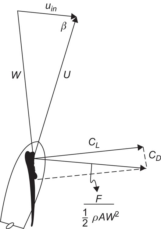
Assuming that C_D, C_L, and W are constant over the area A=∫c dz of the airfoil, the work done by a uniform (except in the vicinity of the airfoil) wind field u_in on a device (e.g., a ship) moving with a velocity U can be derived from (4.58) and (4.59),

$E=\mathit{F}·\mathit{U}.$

The angle β between u_in and U (see Fig. 4.14) may be maintained by a rudder. The power coefficient (4.55) becomes

$C_p=f(C_L\sin \beta -C_D{(1-{\sin }^2\beta +f^2-2f\cos \beta )}^{½}){(1+f^2-2f\cos \beta )}^{½},$

with f=U/u_in. For C_L=0, the maximum C_p is 4C_D/27, obtained for f=1/3 and β=0, whereas the maximum C_p for high lift-to-drag ratios L/D is obtained for β close to 1/2π and f around 2C_L/(3C_D). In this case, the maximum C_p may exceed C_L by one to two orders of magnitude (Wilson and Lissaman, 1974).

It is quite difficult to maintain the high speeds U required for optimum performance in a linear motion of the airfoil, and it is natural to focus the attention on rotating devices, in case the desired energy form is shaft or electric power and not propulsion. Wind-driven propulsion in the past (mostly of ships at sea) has been restricted to U/u_in values far below the optimum region for high L/D airfoils (owing to friction against the water), and wind-driven propulsion on land or in the air has received little attention.

4.3.2.1 Theory of non-interacting streamtubes

In order to describe the performance of a propeller-type rotor, the forces on each element of the blade must be calculated, including the forces produced by the direct action of the wind field on each individual element as well as the forces arising as a result of interactions between different elements on the same or on different blades. Since the simple airfoil theory outlined in section 4.3.1 deals only with the forces on a given blade segment, in the absence of the other ones and also without the inclusion of “edge effects” from “cutting out” this one segment, it is tempting as a first approximation to treat the different radial segments of each blade as independent. Owing to the symmetrical mounting of blades, the corresponding radial segments of different blades (if more than one) may be treated together for a uniform wind field, considering, as indicated in Fig. 4.15, an annulus-shaped streamtube of flow, bordered by streamlines intersecting the rotor plane at radial distances r and r + Dr. The approximation of independent contributions from each streamtube, implying that radially induced velocities (u_r in Fig. 4.10) are neglected, allows the total shaft power to be expressed as

$E={\int }_0^R\frac{\mathrm{d}E}{\mathrm{d}r}dr,$

where dE/dr depends only on the conditions of the streamtube at r. Similar sums of independent contributions can in the same order of approximation be used to describe other overall quantities, such as the axial force component T and the torque Q (equal to the power E divided by the angular velocity Ω of the propeller).

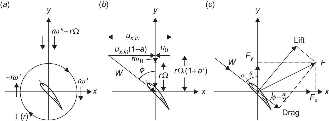
In Fig. 4.16, a section of a wing profile (blade profile) is seen from a direction perpendicular to the cut. The distance of the blade segment from the axis of rotation is r, and its velocity rΩ is directed along the y-axis. This defines a coordinate system with a fixed x-axis along the rotor axis and moving y- and z-axes such that the blade segment is fixed relative to the co-ordinate system.

In order to utilize the method developed in section 4.3.1, the apparent wind velocity W to be used in (4.59) must be determined. It is given by (4.58) only if the velocity induced by, and remaining in the wake of, the device, u^ind=u_out−u_in (cf. Fig. 4.10), is negligible. Since the radial component u_r of u^ind has been neglected, u^ind has two components, one along the x-axis,

${\mathit{u}}_x^{ind}=u_{x,out}-u_{x,in}=-2a{u}_{x,in}$

[cf. (4.52)], and one in the tangential direction,

$u_t^{ind}={\omega }_r^{ind}=2a\prime \mathrm{\Omega }r,$

when expressed in a non-rotating co-ordinate system (the second equality defines a quantity a′, called the tangential interference factor).

W is determined by the air velocity components in the rotor plane. From the momentum considerations underlying (4.52), the induced x-component u₀ in the rotor plane is seen to be

$u_0=1/2u_x^{ind}=-a{u}_{x,in}.$ (4.60)

(4.60)

In order to determine rω₀, the induced velocity of rotation of the air in the rotor plane, one may use the following argument (Glauert, 1935). The induced rotation is partly due to the rotation of the wings and partly due to the non-zero circulation (4.57) around the blade segment profiles (see Fig. 4.16a). This circulation may be considered to imply an induced air velocity component of the same magnitude, |rω′|, but with opposite direction in front of and behind the rotor plane. If the magnitude of the component induced by the wing rotation is called rω″ in the fixed co-ordinate system, it will be rω″ + rΩ and directed along the negative y-axis in the co-ordinate system following the blade. It has the same sign in front of and behind the rotor. The total y-component of the induced air velocity in front of the rotor is then −(rω″ + rΩ + rω′), and the tangential component of the induced air velocity in the fixed co-ordinate system is −(rω″−rω′), still in front of the rotor. But here there should be no induced velocity at all. This follows, for example, from performing a closed line integral of the air velocity v along a circle with radius r and perpendicular to the x-axis. This integral should be zero because the air in front of the rotor has been assumed to be irrotational,

$0={\int }_{circlearea}\mathit{rot}\mathbf{v}dA={\oint }^{}\mathbf{v}·d\mathit{s}=-2\pi r(r\omega ″-r\omega \prime ),$

implying ω″=ω′. This identity also fixes the total induced tangential air velocity behind the rotor, rω^ind=rω″+rω′=2rω″, and in the rotor plane (note that the circulation component rω′ is here perpendicular to the y-axis),

$r{\omega }_0=r\omega ″=1/2r{\omega }^{ind}=\mathrm{\Omega }ra\prime .$ (4.61)

(4.61)

The apparent wind velocity in the co-ordinate system moving with the blade segment, W, is now determined as seen in Fig. 4.16b. Its x-component is u_x, given by (4.52), and its y-component is obtained by taking (4.61) to the rotating co-ordinate system,

$W_x=u_x=u_{x,in}(1-a),$ (4.62a)

(4.62a)

$W_y=-(r{\omega }_x+r\mathrm{\Omega })=-r\mathrm{\Omega }(1+a\prime ).$ (4.62b)

(4.62b)

The lift and drag forces (Fig. 4.16c) are now obtained from (4.61) (except that the two components are no longer directed along the co-ordinate axes), with values of C_D, C_L, and c pertaining to the segments of wings at the streamtube intersecting the rotor plane at the distance r from the axis. As indicated in Figs. 4.16b and c, the angle of attack, α, is the difference between the angle ϕ, determined by

$\tan \varphi =-W_x/W_y,$ (4.63)

(4.63)

and the pitch angle θ between blade and rotor plane,

$\alpha =\varphi -\theta .$ (4.64)

(4.64)

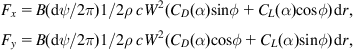
Referred to the co-ordinate axes of Fig. 4.16, the force components for a single blade segment become

$F_x=1/2\rho c{W}^2(C_D(\alpha )\sin \varphi +C_L(\alpha )\cos \varphi ),$ (4.65a)

(4.65a)

$F_y=1/2\rho c{W}^2(-C_D(\alpha )\cos \varphi +C_L(\alpha )\sin \varphi ),$ (4.65b)

(4.65b)

and the axial force and torque contributions from a streamtube with B individual blades are given by

$dT/dr=BF(r),$ (4.66a)

(4.66a)

$dQ/dr=Br{F}_y(r).$ (4.66b)

(4.66b)

Combining (4.66) with equations expressing momentum and angular momentum conservation for each of the (assumed non-interacting) streamtubes, a closed set of equations is obtained. Equating the momentum change of the wind in the x-direction to the axial force on the rotor part intersected by an individual streamtube [i.e., (4.48) and (4.49) with A=2πr], one obtains

$dT/dr=-A\rho u_x{u}_x^{ind}=2\pi r\rho u_{x,in}(1–a)2a{u}_{x,in},$ (4.67)

(4.67)

and similarly equating the torque on the streamtube rotor part to the change in angular momentum of the wind (from zero to r × u^ind_t), one gets

$dQ/dr=A\rho u_x{u}_t^{ind}=2\pi r^2\rho u_{x,in}(1-a)2a\prime \mathrm{\Omega }r.$ (4.68)

(4.68)

Inserting W=u_x,in(1−a)/sin ϕ or W=rΩ (1+a′)/cos ϕ (cf. Fig. 4.16c) as necessary, one obtains a and a′ expressed in terms of ϕ by combining (4.65)–(4.68). Since, on the other hand, ϕ depends on a and a′ through (4.63) and (4.62), an iterative method of solution should be used. Once a consistent set of (a, a′, ϕ)-values has been determined as function of r [using a given blade profile implying known values of θ, c, C_D(α), and C_L(α) as function of r], either (4.66) or (4.67) and (4.68) may be integrated over r to yield the total axial force, total torque, or total shaft power E=Ω Q.

One may also determine the contribution of a single streamtube to the power coefficient (4.55),

$C_p(r)=\frac{\mathrm{\Omega }\mathrm{d}Q/\mathrm{d}r}{½\rho u_{x,in}^{3}2\pi r}=4a\prime (1-a){\left(\frac{r\mathrm{\Omega }}{u_{x,in}}\right)}^2.$ (4.69)

(4.69)

The design of a rotor may utilize C_p(r) for a given wind speed u_x,in^design to optimize the choice of blade profile (C_D and C_L), pitch angle (θ), and solidity (Bc/(πr)) for given angular velocity of rotation (Ω). If the angular velocity Ω is not fixed (as it might be by use of a suitable asynchronous electrical generator, except at start and stop), a dynamic calculation involving dΩ/dt must be performed. Not all rotor parameters need to be fixed. For example, the pitch angles may be variable, by rotation of the entire wing around a radial axis, such that all pitch angles θ (r) may be modified by an additive constant θ₀. This type of regulation is useful in order to limit the C_p-drop when the wind speed moves away from the design value $u_{x.in}^{design}.$ The expressions given above would then give the actual C_p for the actual setting of the pitch angles given by θ (r)_design+θ₀ and the actual wind speed u_x,in, with all other parameters left unchanged.

In introducing the streamtube expressions (4.67) and (4.68), it has been assumed that the induced velocities, and thus a and a′, are constant along the circle periphery of radius r in the rotor plane. As the model used to estimate the magnitude of the induced velocities (Fig. 4.16a) is based on being near to a rotor blade, it is expected that the average induced velocities in the rotor plane, u₀ and rω₀, are smaller than the values calculated by the above expressions, unless the solidity is very large. In practical applications, it is customary to compensate by multiplying a and a′ by a common factor, F, less than unity and a function of B, r, and ϕ (see, for example, Wilson and Lissaman, 1974).

Furthermore, edge effects associated with the finite length R of the rotor wings have been neglected, as have the “edge” effects at r=0 due to the presence of the axis, transmission machinery, etc. These effects may be described in terms of trailing vortices shed from the blade tips and blade roots and moving in helical orbits away from the rotor in its wake. Vorticity is a name for the vector field rotv, and the vortices connected with the circulation around the blade profiles (Fig. 4.16a) are called bound vorticity. This can “leave” the blade only at the tip or at the root. The removal of bound vorticity is equivalent to a loss of circulation I (4.57) and hence a reduction in the lift force. Its dominant effect is on the tangential interference factor a′ in (4.68), and so it has the same form and may be treated on the same footing as the corrections due to finite blade number. (Both are often referred to as tip losses, since the correction due to finite blade number is usually appreciable only near the blade tips, and they may be approximately described by the factor F introduced above.) Other losses may be associated with the “tower shadow,” etc.

4.3.2.2 Model behavior of power output and matching to load

A calculated overall C_p for a three-bladed, propeller-type wind energy converter is shown in Fig. 4.17, as a function of the tip-speed ratio,

$\lambda =\mathrm{\Omega }R/u_{x,in},$

and for different settings of the overall pitch angle, θ₀. It is clear from (4.69) and the equations for determining a and a′ that C_p depends on the angular velocity Ω and the wind speed u_x,in only through the ratio λ. Each blade has been assumed to be an airfoil of the type NACA 23012 (cf. Fig. 4.12), with chord c and twist angle θ changing along the blade from root to tip, as indicated in Fig. 4.18. A tip-loss factor F has been included in the calculation of sets of corresponding values of a, a′, and ϕ for each radial station (each “streamtube”), according to the Prandtl model described by Wilson and Lissaman (1974). The dashed regions in Fig. 4.17 correspond to values of the product aF (corresponding to a in the expression without tip loss) larger than 0.5. Since the axial air velocity in the wake is u_x,out=u_x,in(1−2 aF) [cf. (4.52) with F=1], aF > 0.5 implies reversed or re-circulating flow behind the wind energy converter, a possibility that has not been included in the above description. The C_p values in the dashed regions may thus be inaccurate and presumably overestimated.

Figure 4.17 shows that, for negative settings of the overall pitch angle θ₀, the C_p distribution on λ values is narrow, whereas it is broad for positive θ₀ of modest size. For large positive θ₀, the important region of C_p moves to smaller λ values. The behavior of C_p(λ) in the limit of λ approaching zero is important for operating the wind energy converter at small rotor angular velocities and, in particular, for determining whether the rotor will be self-starting, as discussed in more detail below.

For a given angular speed Ω of the rotor blades, the power coefficient curve specifies the fraction of the power in the wind that is converted, as a function of the wind speed u_x,in. Multiplying C_p by $1/2\rho A{u}_{x.in,}^3$ where the rotor area is A=πR² (if “coning” is disregarded, i.e., the blades are assumed to be in the plane of rotation), the power transferred to the shaft can be obtained as a function of wind speed, assuming the converter to be oriented (“yawed”) such that the rotor plane is perpendicular to the direction of the incoming wind. Figures 4.19 and 4.20 show such plots of power E, as functions of wind speed and overall pitch angle, for two definite angular velocities (Ω=4.185 and 2.222 rad s⁻¹, if the length of the wings is R=27 m). For the range of wind speeds encountered in the planetary boundary layer of the atmosphere (e.g., at heights between 25 and 100 m), a maximum power level around 4000 W per average square meter swept by the rotor (10 MW total) is reached for the device with the higher rotational speed (tip speed RΩ=113 Ms⁻¹), whereas about 1000 W m⁻² is reached by the device with the lower rotational velocity (RΩ=60 m s⁻¹).

The rotor has been designed to yield a maximum C_p at about λ=9 (Fig. 4.17), corresponding to u_x,in=12.6 and 6.6 m s⁻¹ in the two cases. At wind speeds above these values, the total power varies less and less strongly, and for negative pitch angles it even starts to decrease with increasing wind speeds in the range characterizing “stormy weather.” This phenomenon can be used to make the wind energy converter self-regulating, provided that the “flat” or “decreasing” power regions are suitably chosen and that the constancy of the angular velocity at operation is ensured by, for example, coupling the shaft to a suitable asynchronous electricity generator (a generator allowing only minute changes in rotational velocity, with the generator angular speed Ω_g being fixed relative to the shaft angular speed Ω, e.g., by a constant exchange ratio n=Ω_g/Ω of a gearbox). Self-regulating wind energy converters with fixed overall pitch angle θ₀ and constant angular velocity have long been used for AC electricity generation (Juul, 1964).

According to its definition, the torque Q=E/Ω can be written

$Q=1/2\rho \pi R^3{u}_{x,in}^2{C}_p(\lambda )/\lambda ,$ (4.70)

(4.70)

and Fig. 4.21 shows C_p/λ as a function of λ for the same design as the one considered in Fig. 4.17. For pitch angles θ₀ less than about −3°, C_p/λ is negative for λ=0, whereas the value is positive if θ₀ is above the critical value of about −3°. The corresponding values of the total torque (4.70), for a rotor with radius R=27 m and overall pitch angle θ₀=0°, are shown in Fig. 4.22a, as a function of the angular velocity Ω=λu_x,in/R and for different wind speeds. The small dip in Q for low rotational speeds disappears for higher pitch angles θ₀.

The dependence of the torque at Ω=0 on pitch angle is shown in Fig. 4.23 for a few wind speeds. Advantage can be taken of the substantial increase in starting torque with increasing pitch angle, in case the starting torque at the pitch angle desired at operating angular velocities is insufficient and provided the overall pitch angle can be changed. In that case, a high overall pitch angle is chosen to start the rotor from Ω=0, where the internal resistance (friction in bearings, gearbox, etc.) is large. When an angular speed Ω of a few degrees per second is reached, the pitch angle is diminished to a value close to the optimal one (otherwise the torque will pass a maximum and soon start to decrease again, as seen from, for example, the θ₀=60° curve in Fig. 4.21). Usually, the internal resistance diminishes as soon as Ω is non-zero. The internal resistance may be represented by an internal torque, Q₀(Ω), so that the torque available for some load, “external” to the wind power to shaft power converter (e.g., an electric generator), may be written

$Q^{available}=Q(\mathrm{\Omega })-Q_0(\mathrm{\Omega }).$

If the “load” is characterized by demanding a fixed rotational speed Ω (such as the asynchronous electric generator), it may be represented by a vertical line in the diagram shown in Fig. 4.22a. As an example of the operation of a wind energy generator of this type, the dashed lines (with accompanying arrows) in Fig. 4.22a describe a situation with initial wind speed of 8 m s⁻¹, assuming that this provides enough torque to start the rotor at the fixed overall pitch angle θ₀=0° (i.e., the torque produced by the wind at 8 m s⁻¹ and Ω=0 is above the internal torque Q₀, here assumed to be constant). The excess torque makes the angular velocity of the rotor, Ω, increase along the specific curve for u_x,in=8 m s⁻¹, until the value Ω₀ characterizing the electric generator is reached. At this point, the load is connected and the wind energy converter begins to deliver power to the load area. If the wind speed later increases, the torque will increase along the vertical line at Ω=Ω₀ in Fig. 4.22a, and if the wind speed decreases, the torque will decline along the same vertical line until it reaches the internal torque value Q₀. Then the angular velocity diminishes and the rotor is brought to a halt.

An alternative type of load may not require a constant angular velocity. Synchronous DC electric generators are of this type, providing an increasing power output with increasing angular velocity (assuming a fixed exchange ratio between rotor angular velocity Ω and generator angular velocity Ω_g). Instead of staying on a vertical line in the torque-versus-Ω diagram, for varying wind speed, the torque now varies along some fixed, monotonically increasing curve characterizing the generator. An optimal synchronous generator would be characterized by a Q(Ω) curve that for each wind speed u_x,in corresponds to the value of Ω=λu_x,in/R that provides the maximum power coefficient C_p (Fig. 4.17). This situation is illustrated in Fig. 4.22b, with a set of dashed curves again indicating the torque variation for an initial wind speed of 8 m s⁻¹, followed by an increasing and later again decreasing wind speed. In this case, the Q=Q₀ limit is finally reached at a very low angular velocity, indicating that power is still delivered during the major part of the slowing-down process.

4.3.2.3 Non-uniform wind velocity

The velocity field of the wind may be non-uniform in time as well as in spatial distribution. The influence of time variations in wind speed on power output of a propeller-type wind energy converter is touched upon in the previous subsection, although a detailed investigation involving the actual time dependence of the angular velocity Ω is not included. In general, the direction of the wind velocity is also time dependent, and the conversion device should be able to successively align its rotor axis with the long-range trends in wind direction, or suffer a power reduction that is not just the cosine to the angle β between the rotor axis and the wind direction (yaw angle), but involves calculating the performance of each blade segment for an apparent wind speed W and angle of attack α different from the ones previously used, and no longer axially symmetric. This means that the quantities W and α (or ϕ) are no longer the same inside a given annular streamtube, but they depend on the directional position of the segment considered (e.g., characterized by a rotational angle ϕ in a plane perpendicular to the rotor axis).

Assuming that both the wind direction and the wind speed are functions of time and of height h (measured from ground level or from the lower boundary of the velocity profile z₀ discussed in section 2.5.2), but that the direction remains horizontal, then the situation will be as depicted in Fig. 4.24. The co-ordinate system (x₀, y₀, z₀) is fixed and has its origin in hub height h₀, where the rotor blades are fastened. Consider now a blade element at a distance r from the origin, on the ith blade. The projection of this position on to the (y₀, z₀)-plane is turned the angle ψ_i from vertical, where

${\psi }_i=2\pi /i+\mathrm{\Omega }t,$ (4.71)

(4.71)

at the time t. The coning angle δ is the angle between the blade and its projection onto the (y₀, z₀)-plane, and the height of the blade element above the ground is

$h=h_0+r\cos \delta \cos {\psi }_i,$ (4.72)

(4.72)

where h₀ is the hub height. The height h enters as a parameter in the wind speed u_in=ju_in(h, t)j and the yaw angle β=β (h, t), in addition to time.

Now, an attempt can be made to copy the procedure used for a uniform wind velocity along the rotor axis, i.e., to evaluate the force components for an individual streamtube both by the momentum consideration and by the lift and drag approach of section 4.3.1. The individual streamtubes can no longer be taken as annuli, but must be of an area A_s (perpendicular to the wind direction) small enough to permit the neglect of variations in wind velocity over the area at a given time. It will still be assumed that the flows inside different streamtubes do not interact, and also, for simplicity, the streamtubes will be treated as “straight lines,” i.e., not expanding or bending as they pass the region of the conversion device (as before, this situation arises when induced radial velocities are left out).

Consider first the “momentum equation” (4.48), with s denoting “in the streamwise direction” or “along the streamtube,”

$F_s=-J_m{u}_s^{ind}.$

This force has components along the x-, y-, and z-directions of the local coordinate system of a blade turned the angle ψ from vertical (cf. Fig. 4.69). The y-direction is tangential to the rotation of the blade element, and, in addition to the component of F_s, there may be an induced tangential velocity u_t^ind (and force) of the same type as the one considered in the absence of yaw (in which case F_s is perpendicular to the y-axis). The total force components in the local co-ordinate system are thus

$\begin{array}{ll}{F}_x\hfill & =-J_m{u}_s^{ind}(\cos \beta \cos \delta +\sin \beta \sin \delta \sin \psi ),\hfill \\ F_y\hfill & =-J_m{u}_s^{ind}\sin \beta \cos \psi +J_m{u}_t^{ind}.\hfill \end{array}$ (4.73)

(4.73)

From the discussion of Fig. 4.10, (4.49) and (4.52),

$\begin{array}{ll}{J}_m\hfill & =A_s\rho u_s=A_s\rho u_{in}(1-a),\hfill \\ u_s^{ind}\hfill & =-2a{u}_{in},\hfill \end{array}$

and, in analogy with (4.61), a tangential interference factor a′ may be defined by

$u_t^{ind}=2a\prime r\mathrm{\Omega }\cos \delta .$

However, the other relation contained in (4.61), from which the induced tangential velocity in the rotor plane is half the one in the wake, cannot be derived in the same way without the assumption of axial symmetry. Instead, the variation in the induced tangential velocity as a function of rotational angle ψ is bound to lead to crossing of the helical wake strains and it will be difficult to maintain the assumption of non-interacting streamtubes. Here, the induced tangential velocity in the rotor plane will still be taken as 1/2u_t^ind, an assumption which at least gives reasonable results in the limiting case of a nearly uniform incident wind field and zero or very small yaw angle.

Secondly, the force components may be evaluated from (4.63) to (4.65) for each blade segment, defining the local co-ordinate system (x, y, z) as in Fig. 4.24 with the z-axis along the blade and the y-axis in the direction of the blade’s rotational motion. The total force, averaged over a rotational period, is obtained by multiplying by the number of blades, B, and by the fraction of time each blade spends in the streamtube. Defining the streamtube dimensions by an increment Dr in the z-direction and an increment dψ in the rotational angle ψ, each blade spends the time fraction dψ/(2π) in the streamtube, at constant angular velocity Ω. The force components are then

$\begin{array}{cc}{F}_x& =B(\mathrm{d}\psi /2\pi )1/2\rho \mathit{c}{\mathit{W}}^2(C_D(\alpha )\sin \varphi +C_L(\alpha )\cos \varphi )\mathrm{d}r,\\ F_y& =B(\mathrm{d}\psi /2\pi )1/2\rho \mathit{c}{\mathit{W}}^2(C_D(\alpha )\cos \varphi +C_L(\alpha )\sin \varphi )\mathrm{d}r,\end{array}$ (4.74)

(4.74)

in the notation of (4.65). The angles ϕ and α are given by (4.63) and (4.64), but the apparent velocity W is the vector difference between the streamwise velocity u_in+1/2 u_s^ind and the tangential velocity rΩ cos δ+1/2 u_t^ind, both taken in the rotor plane. From Fig. 4.24,

$\begin{array}{ll}{W}_x\hfill & =u_{in}(1-a)(\cos \beta \cos \delta +\sin \beta \sin \delta \sin \psi ),\hfill \\ W_y\hfill & =u_{in}(1-a)\sin \beta \cos \psi +r\mathrm{\Omega }\cos \delta (1+a\prime ),\hfill \\ W_z\hfill & =u_{in}(1-a)(-\cos \beta \sin \delta +\sin \beta \cos \delta \sin \psi ).\hfill \end{array}$ (4.75)

(4.75)

The appropriate W² to insert into (4.74) is W_x²+W_y². Finally, the relation between the streamtube area A_s and the increments Dr and dψ must be established. As indicated in Fig. 4.25, the streamtube is approximately a rectangle with sides dL and dL′, given by

$\begin{array}{ll}\mathrm{d}L\hfill & =r\cos \delta {(\cos 2\beta \cos 2\psi +\sin 2\psi )}^{1/2}\mathrm{d}\psi \hfill \\ \mathrm{d}L″\hfill & ={(\sin 2\delta (1+\cos 2\beta )+\cos 2\delta (\cos 2\beta \sin 2\psi +\cos 2\psi ))}^{1/2}\mathrm{d}r,\hfill \end{array}$ (4.76)

(4.76)

and

$A_s=dLdL\prime .$

Now, for each streamtube, a and a′ are obtained by equating the x- and y-components of (4.73) and (4.74) and using the auxiliary equations for (W, ϕ) or (W_x, W_y). The total thrust and torque are obtained by integrating F_x and r cos δ F_y, over Dr and dψ (i.e., over all streamtubes).

4.3.2.4 Restoration of wind profile in wake, and implications for turbine arrays

For a wind energy converter placed in the planetary boundary layer (i.e., in the lowest part of the Earth’s atmosphere), the reduced wake wind speed in the streamwise direction, u_s,out, will not remain below the wind speed u_s,in of the initial wind field, provided that this is not diminishing with time. The processes responsible for maintaining the general kinetic motion in the atmosphere (cf. section 2.3.1), making up for the kinetic energy lost by surface friction and other dissipative processes, will also act in the direction of restoring the initial wind profile (speed as function of height) in the wake of a power-extracting device by transferring energy from higher air layers (or from the “sides”) to the partially depleted region (Sørensen, 1996). The large amounts of energy available at greater altitude (cf. Fig. 3.31) make such processes possible almost everywhere at the Earth’s surface and not just at those locations where new kinetic energy is predominantly being created (cf. Fig. 2.60).

In the near wake, the wind field is non-laminar, owing to the induced tangential velocity component, u_t^ind, and owing to vorticity shed from the wing tips and the hub region (cf. discussion of Figs. 4.16 and (4.57)). It is then expected that these turbulent components gradually disappear further downstream in the wake, as a result of interactions with the random eddy motion of different scales present in the “unperturbed” wind field. “Disappear” here means “get distributed on a large number of individual degrees of freedom,” so that no contributions to the time-averaged quantities considered [cf. (2.21)] remain. For typical operation of a propeller-type wind conversion device, such as the situations illustrated in Figs. 4.19 and 4.20, the tangential interference factor a′ is small compared to the axial interference factor a, implying that the most visible effect of the passage of the wind field through the rotor region is the change in streamwise wind speed. Based on wind tunnel measurements, this is a function of r, the distance of the blade segment from the hub center, as illustrated in Fig. 4.27. The induced r-dependence of the axial velocity is seen to gradually smear out, although it is clearly visible at a distance of two rotor radii in the set-up studied.

Fig. 4.28 suggests that, under average atmospheric conditions, the axial velocity, u_s,in, will be restored to better than 90% at about 10 rotor diameters behind the rotor plane and better than 80% at a distance of 5–6 rotor diameters behind the rotor plane, but restoration is rather strongly dependent on the amount of turbulence in the “undisturbed” wind field.

A second wind energy converter may be placed behind the first one, in the wind direction, at a location where the wind profile and magnitude are reasonably well restored. According to simplified investigations in wind tunnels (Fig. 4.28), supported by field measurements behind buildings, forests, and fences, a suitable distance would seem to be 5–10 rotor diameters (increasing to over 20 rotor diameters if “complete restoration” is required). If there is a prevailing wind direction, the distance between conversion units perpendicular to this direction may be smaller (essentially determined by the induced radial velocities, which were neglected in the preceding subsections, but appear qualitatively in Fig. 4.10). If, on the other hand, several wind directions are important, and the converters are designed to be able to “yaw against the wind,” then the distance required by wake considerations should be kept in all directions.

More severe limitations may possibly be encountered with a larger array of converters, say, distributed over an extended area with average spacing X between units. Even if X is chosen so that the relative loss in streamwise wind speed is small from one unit to the next, the accumulated effect may be substantial, and the entire boundary layer circulation may become altered in such a way that the power extracted decreases more sharply than expected from the simple wake considerations. Thus, large-scale conversion of wind energy may even be capable of inducing local climatic changes.

A detailed investigation of the mutual effects of an extended array of wind energy converters and the general circulation on each other requires a combination of a model of the atmospheric motion, e.g., along the lines presented in section 2.3.1, with a suitable model of the disturbances induced in the wake of individual converters. In one of the first discussions of this problem, Templin (1976) considered the influence of an infinite two-dimensional array of wind energy converters with fixed average spacing on the boundary layer motion to be restricted to a change of the roughness length z₀ in the logarithmic expression (see section 2.5.1) for the wind profile, assumed to describe the wind approaching any converter in the array. The change in z₀ can be calculated from the stress τ^ind exerted by the converters on the wind, due to the axial force F_x in (4.65) or (4.67), which according to (4.51) can be written

${\tau }^{ind}=F_x/S=1/2\rho {(u_{s,in})}^{2}2{(1-a)}^{2}A/S,$

with S being the average ground surface area available for each converter and A/S being the “density parameter,” equal to the ratio of rotor-swept area to ground area. For a quadratic array with regular spacing, S may be taken as X². According to section 2.5.1, u_x,in taken at hub height h₀ can, in the case of a neutral atmosphere, be written

$u_{x,in}(h_0)=\frac{1}{\kappa }{\left(\frac{{\tau }^0+{\tau }^{ind}}{\rho }\right)}^{1/2}\log \left(\frac{h_0}{z{\prime }_0}\right),$

where τ⁰ is the stress in the absence of wind energy converters, and z′₀ is the roughness length in the presence of the converters, which can now be determined from this equation and τ^ind from the previous one.

Figure 4.29 shows the results of a calculation for a finite array of converters (Taylor et al., 1993) using a simple model with fixed loss fractions (Jensen, 1994). This model is incapable of reproducing the fast restoration of winds through the turbine array, presumably associated with the propagation of the enhanced wind regions created just outside the swept areas (as seen in Fig. 4.27). A three-dimensional fluid dynamics model is required for describing the details of array shadowing effects. Such calculations are in principle possible, but so far no convincing implementation has been presented. The problem is the very accurate description needed for the complex three-dimensional flows around the turbines and for volumes comprising the entire wind farm of maybe hundreds of turbines. This is an intermediate regime between the existing three-dimensional models for gross wind flow over complex terrain and the detailed models of flow around a single turbine used in calculations of aerodynamic stability.

4.3.2.5 Size limits

Horizontal axis, propeller-type wind generators have increased in size with time, and by 2016, the largest commercial turbines have rotor diameters of around 160 m (4C Offshore Consultancy UK, 2016). Although fiber materials can be produced with strengths sufficient to further increase the blade length, the weight of the part of the blades furthest from the hub is becoming a problem and efforts are ongoing partly to find new ultralight materials of high strength, and partly to reconsider the blade geometry and the inside reinforcement required for making a hollow blade strong and durable. Making the width of the blade decrease faster toward the end is one solution, even if it may compromise the most efficient profile selection. Material choice and design of the inside reinforcement is another optimization feature studied with the purpose of maintaining the necessary strength and yet keeping weight down. Figure 4.26 shows the cross section of a design currently favored, and a model calculation for determining the optimum way of placing the mass of blade materials (Forcier and Joncas, 2012). However, it is not unlikely that a practical limit to blade length is in sight, because at some point, increasing the rotor diameter of a horizontal axis turbine may not entail any economic advantage, even if it could be achieved by introducing new technical ideas. In the United States, an ongoing project is exploring the possibility of using blade materials much more flexible (allowed to bend substantially) than those of current technology, and with hinges allowing the blades to lie flat along the wind direction at high wind speeds (ARPA-E, 2015; Griffith, 2016). One may worry that the ease of bending contributes to giving such blades a shorter life. Blades for wind turbines are supposed to last for some 25 years, which leaves little room for frequent large-amplitude bending at the current level of materials technology.

4.3.2.6 Floating offshore wind turbines

One of the first suggestions to place wind turbines at the higher winds (see Fig. 6.30) found offshore was made by Musgrove (1978). Implementation started in Denmark during the 1990s. While current offshore wind arrays are sitting on foundations, it has been suggested to use floating wind turbines placed at water depths too large for foundations. Tests of various designs for buoyancy stabilization (platforms, cylinders, mooring, anchors) have been ongoing in Europe and Japan (Anonymous, 2016a), based on floating platforms for oil and gas extraction. Whether and under what conditions the cost implications are favorable remains to be seen. The same issue has been discussed for oil and gas platforms, where the main advantage of avoiding foundation is stated to be that the same floating structure design can be used everywhere. This would not seem relevant for wind farms, where the economy of mass production is anyway present due to the usually over 100 turbines installed within each farm.

4.3.2.7 Offshore foundation issues

The current surge in power plants with wind turbines placed offshore, typically in shallow waters of up to 50 m depth, relies on the use of low-cost foundation methods developed earlier for harbor and oil-well uses. The best design depends on the material constituting the local water floor, as well as local hydrological conditions, including strength of currents and icing problems. Breakers are currently used to prevent ice from damaging the structure. The most common structures in place today are shown in Fig. 4.30: a concrete caisson (Fig. 4.30a) or the steel cylinder solutions shown in Fig. 4.30b and c. The monopile solution (Fig. 4.30c) has been selected for several recent projects such as the Samsø wind farm in the middle of Denmark (Birck and Gormsen, 1999; Offshore Windenergy Europe, 2003). Employing the sea-bed suction effect (Fig. 4.30b) may help cope with short-term gusting forces, while the general stability must be ensured by the properties of the overall structure itself. The option of offshore deployment is of course relevant not just for horizontal axis machines but for all types of wind converters, including those described below in section 4.3.3.

4.3.3.1 Performance of a Darrieus-type converter

The performance of a cross-wind converter, such as the Darrieus rotor shown in Fig. 4.31, may be calculated in a way similar to that used in section 4.3.2, deriving the unknown, induced velocities by comparing expressions of the forces in terms of lift and drag on the blade segments with expressions in terms of the momentum changes between incident wind and wake flow. In addition, the flow may be divided into a number of streamtubes (assumed to be non-interacting), according to assumptions about the symmetries of the flow field. Figure 4.21 gives an example of the streamtube definitions for a two-bladed Darrieus rotor with angular velocity Ω and a rotational angle ψ describing the position of a given blade, according to (4.71). The blade chord, c, has been illustrated as constant, although it may actually be taken as varying to give the optimum performance for any blade segment at the distance r from the rotor axis. As in the propeller rotor case, it is not practical to extend the chord increase to the regions near the axis.

The bending of the blade, characterized by an angle δ (h) depending on the height h (the height of the rotor center is denoted h₀), may be taken as a troposkien curve (Blackwell and Reis, 1974), characterized by the absence of bending forces on the blades when they are rotating freely. Since the blade profiles encounter wind directions at both positive and negative forward angles, the profiles are often taken as symmetrical (e.g., NACA 00XX profiles).

Assuming, as in section 4.3.2, that the induced velocities in the rotor region are half of those in the wake, the streamtube expressions for momentum and angular momentum conservation analogous to (4.67) and (4.68) are

$\begin{array}{ll}{F}_{x0}\hfill & =-J_m{u}_s^{ind}=2\rho A_s{(u_{in})}^2(1-a)a,\hfill \\ F_{y0}\hfill & =J_m{u}_{c.w.}^{ind},\hfill \end{array}$ (4.77)

(4.77)

where the axial interference factor a is defined as in (4.60), and where the streamtube area A_s corresponding to height and angular increments dh and dψ is (cf. Fig. 4.31)

$A_s=r\sin \psi \mathrm{d}\psi dh.$

The cross wind–induced velocity $u_{c.w}^{ind}$ is not of the form (4.61), since the tangent to the blade’s rotational motion is not along the y₀-axis. The sign of $u_{c.w}^{ind}$ will fluctuate with time and for low chordal ratio c/R (R being the maximum value of r) it may be permitted to put F_y0 equal to zero (Lissaman, 1976; Strickland, 1975). This approximation is made in the following. It is also assumed that the streamtube area does not change by passage through the rotor region and that individual streamtubes do not interact (these assumptions being the same as those made for the propeller-type rotor).

The forces along the instantaneous x- and y-axes due to the passage of the rotor blades at a fixed streamtube location (h, ψ) can be expressed in analogy to (4.74), averaged over one rotational period,

$F_x=B(d\psi /2\pi )1/2\rho c{W}^2(C_D\sin \varphi +C_L\cos \varphi )\mathrm{d}h/\cos \delta ,$ (4.78a)

(4.78a)

$F_y=B(d\psi /2\pi )1/2\rho c{W}^2(-C_D\cos \varphi +C_L\sin \varphi )\mathrm{d}h/\cos \delta ,$ (4.78b)

(4.78b)

where

$\tan \varphi =-W_x/W_y;W^2=W_x^2+W_y^2$

and (cf. Fig. 4.21)

$\begin{array}{ll}{W}_x\hfill & =u_{in}(1-a)\sin \psi \cos \delta ,\hfill \\ W_y\hfill & =-r\mathrm{\Omega }-u_{in}(1-a)\cos \psi ,\hfill \\ W_z\hfill & =-u_{in}(1-a)\sin \psi \sin \delta .\hfill \end{array}$ (4.79)

(4.79)

The angle of attack is still given by (4.64), with the pitch angle θ being the angle between the y-axis and the blade center chord line (cf. Fig. 4.16c).

The force components (4.78) may be transformed to the fixed (x₀, y₀, z₀) co-ordinate system, yielding

$F_{x0}=F_x\cos \delta \sin \psi +F_y\cos \psi ,$ (4.80)

(4.80)

with the other components F_y0 and F_z0 being neglected due to the assumptions made. Using the auxiliary relations given, a may be determined by equating the two expressions (4.77) and (4.80) for F_x0.

After integration over dh and dψ, the total torque Q and power coefficient C_p can be calculated. Figure 4.32 gives an example of the calculated C_p for a low-solidity, two-bladed Darrieus rotor with NACA 0012 blade profiles and a size corresponding to Reynolds number Re=3 × 10⁶. The curve is similar to the ones obtained for propeller-type rotors (e.g., Fig. 4.17), but the maximum C_p is slightly lower. The reasons why this type of cross-wind converter cannot reach the maximum C_p of 16/27 derived from (4.55) (the “Betz limit”) are associated with the fact that the blade orientation cannot remain optimal for all rotational angles ψ_i, as discussed (in terms of a simplified solution to the model presented above) by Lissaman (1976).

Figure 4.33 gives the torque as a function of angular velocity Ω for a small three-bladed Darrieus rotor. When compared with the corresponding curves for propeller-type rotors shown in Fig. 4.22a and b (or generally Fig. 4.21), it is evident that the torque at Ω=0 is zero for the Darrieus rotor, implying that it is not self-starting. For application with an electric grid or some other back-up system, this is no problem, since the auxiliary power needed to start the Darrieus rotor at the appropriate times is very small compared with the wind converter output, on a yearly average basis. However, for application as an isolated source of power (e.g., in rural areas), it is a disadvantage, and it has been suggested that a small Savonius rotor should be placed on the main rotor axis in order to provide the starting torque (Banas and Sullivan, 1975).

Another feature of the Darrieus converter (as well as of some propeller-type converters), which is evident from Fig. 4.33, is that for application with a load of constant Ω (as in Fig. 4.22a), there will be a self-regulating effect, in that the torque will rise with increasing wind speed only up to a certain wind speed. If the wind speed increases further, the torque will begin to decrease. For variable-Ω types of load (as in Fig. 4.22b), the behavior of the curves in Fig. 4.33 implies that cases of irregular increase and decrease of torque, with increasing wind speed, can be expected.

4.3.3.2 Multiple rotor configurations

Placing more than one rotor on the same tower is an old idea, first forwarded by Juul (1964), arguing that two rotors placed at different positions vertically could cater to both lower and higher wind speeds. In 2016, the company Vestas is testing a prototype 4-rotor design (in a square configuration of two horizontally by two vertically), suggesting that for onshore applications this might be less expensive per unit of energy produced than using one large rotor. Again the output of the bottom rotors will, due to obstacles to wind flow (roughness, buildings, forests, fences and so on), be low, but perhaps gaining more operating hours over the year, if the blades are suitable designed (Anonymous, 2016b).

4.3.3.3 Augmenters and other “advanced” converters

In the preceding sections, it has been assumed that the induced velocities in the converter region were half of those in the wake. This is strictly true for situations where all cross-wind induced velocities (u_t and u_r) can be neglected, as shown in (4.50), but if suitable cross-wind velocities can be induced so that the total streamwise velocity in the converter region, u_x, exceeds the value of −1/2(u_x,in + u_x,out) by a positive amount δu_x^ind, then the Betz limit on the power coefficient, C_p=16/27, may be exceeded,

$u_x=1/2(u_{x,in}+u_{x,out})+\delta u_x^{ind}.$

A condition for this to occur is that the extra induced streamwise velocity δ u_x^ind does not contribute to the induced velocity in the distant wake, u_x^ind, which is given implicitly by the above form of u_x, since

$u_{x,out}=u_{x,in}+u_x^{ind}=u_{x,in}(1-2a).$

The streamtube flow at the converter, (4.49), is then

$J_m=\rho A_s{u}_x=\rho A_s{u}_{x,in}(1-a+ã)$ (4.81)

(4.81)

with $\tilde{a}=\delta u_x^{ind}/u_{x,in},$ and the power (4.53) and power coefficient (4.55) are replaced by

$\begin{array}{ll}E\hfill & =\rho A_s{(u_{x,in})}^{3}2a(1-a)(1-a+\tilde{a}),\hfill \\ C_p\hfill & =4a(1-a)(1-a+\tilde{a}),\hfill \end{array}$ (4.82)

(4.82)

where the streamtube area A_s equals the total converter area A, if the single-streamtube model is used.

4.3.6.1 Heat, electrical/mechanical power, and fuel generation

The wind energy converters described in the preceding sections primarily convert the power in the wind into rotating shaft power. The conversion system generally includes a further conversion step if the desired energy form is different from that of the rotating shaft.

Examples of this are electric generators with fixed or variable rotational velocity, mentioned in connection with Fig. 4.22a and b. The other types of energy can, in most cases, be obtained by secondary conversion of electric power. In some such cases, the “quality” of electricity need not be as high as that usually maintained by utility grid systems, in respect to voltage fluctuations and variations in frequency in the (most widespread) case of alternating current (AC). For wind energy converters aimed at constant working angular velocity Ω, it is customary to use a gearbox and an induction-type generator. This maintains an AC frequency equal to that of the grid and constant to within about 1%. Alternatively, the correct frequency can be prescribed electronically. In both cases, reactive power is created (i.e., power that, like that of a condenser or coil, is phase shifted), which may be an advantage or disadvantage, depending on the loads on the grid.

For variable-frequency wind energy converters, the electric output would be from a synchronous generator and in the form of variable-frequency AC. This would have to be subjected to a time-dependent frequency conversion, and for arrays of wind turbines, phase mismatch would have to be avoided. Several schemes exist for achieving this, for example, semiconductor rectifying devices (thyristors), which first convert the variable frequency AC to DC (direct current) and then, in a second step, the DC to AC of the required fixed frequency.

If the desired energy form is heat, “low-quality” electricity may first be produced, and the heat may then be generated by leading the current through a high ohmic resistance. Better efficiency can be achieved if the electricity can be used to drive the compressor of a heat pump (see section 4.2.3), taking the required heat from a reservoir of temperature lower than the desired one. It is also possible to convert the shaft power more directly into heat. For example, the shaft power may drive a pump, pumping a viscous fluid through a nozzle, so that the pressure energy is converted into heat. Alternatively, the shaft rotation may be used to drive a “paddle” through a fluid, in such a way that large drag forces arise and the fluid is put into turbulent motion, gradually dissipating the kinetic energy into heat. If water is used as the fluid medium, the arrangement is called a water-brake.

Windmill shaft power has traditionally been used to perform mechanical work of various kinds, including flour milling, threshing, lifting, and pumping. Pumping of water (e.g., for irrigation purposes), with a pump connected to the rotating shaft, may be particularly suitable as an application of wind energy, since variable and intermittent power would, in most cases, be acceptable, as long as the average power supply, in the form of lifted water over an extended period of time, is sufficient.

In other cases, an auxiliary source of power may be needed, so that demand can be met at any time. For grid-based systems, this can be achieved by trade of energy (cf. scenarios described in Chapter 6). Demand matching can also be ensured if an energy storage facility of sufficient capacity is attached to the wind energy conversion system. A number of such storage facilities are mentioned in Chapter 5, and among them is the storage of energy in the form of fuels, such as hydrogen. Hydrogen may be produced, along with oxygen, by electrolysis of water, using electricity from the wind energy converter. The detailed working of these mechanisms over time and space is simulated in the scenarios outlined in Chapter 6 and related studies (Sørensen et al., 2004; Sørensen, 2015).

The primary interest may also be oxygen, for example, to be dissolved into the water of lakes that are deficient in oxygen (say, as a result of pollution), or to be used in connection with “ocean farming,” where oxygen may be a limiting factor if nutrients are supplied in large quantities, e.g., by artificial upwelling. The oxygen may be supplied by wind energy converters with reverse-mode fuel cells, while the co-produced hydrogen may be used to produce or move the nutrients. Again, in this type of application, large power fluctuations may be acceptable.

4.3.9.1 Pneumatic converter

The only wave energy conversion device that has been in considerable practical use, although on a fairly small scale, is the buoy of Masuda (1971), shown in schematic form in Fig. 4.41. Several similar wave-power devices exist, based on an oscillating water column driving an air turbine; in some cases, they are shore-based and have only one chamber (see, for example, CRES, 2002). The buoy in Fig. 4.41 contains a tube extending downward, into which water can enter from the bottom, and a “double-action” air turbine, i.e., a turbine that turns the same way under the influence of both pressure and suction (as illustrated by the non-return valves).

Wave motion will cause the whole buoy to move up and down and thereby create an up-and-down motion of the water level in the center tube, which in turn produces the pressure increases and decreases that make the turbine in the upper air chamber rotate. Special nozzles may be added to increase the speed of the air impinging on the turbine blades.

For a simple sinusoidal wave motion, as described in section 2.5.3, but omitting the viscosity-dependent exponential factor, the variables σ₁ and Z, describing the water level in the center tube and the vertical displacement of the entire buoy, respectively, may also be expected to vary sinusoidally, but with phase delays and different amplitudes,

$\begin{array}{ll}\sigma \hfill & =a\cos (kx-\omega t),\hfill \\ {\sigma }_1\hfill & ={\sigma }_{10}\cos (kx-\omega t-{\delta }_{\sigma }),\hfill \\ Z\hfill & =Z_0\cos (kx-\omega t-{\delta }_Z),\hfill \end{array}$

with ω=kU_w in terms of the wave number k and phase velocity U_w (cf. section 2.5.3). The relative air displacement ρ₁ in the upper part of the center tube (the area of which is $A_1=\pi R_1^2$) is now (see Fig. 4.41)

${\rho }_1={\sigma }_1-Z.$

Assuming the airflow incompressible, continuity requires that the relative air velocity dρ₂/dt in the upper tubes forming the air chamber (of area $A_1=\pi R_2^2$) be

$\mathrm{d}{\rho }_2/\mathrm{d}t=(A_1/A_2)\mathrm{d}{\rho }_1/\mathrm{d}t.$

It is now possible to set up the equations of motion for σ₁ and Z, equating the accelerations d²σ₁/dt² and d²Z/dt² multiplied by the appropriate masses (of the water column in the center tube and of the entire device) to the sum of forces acting on the mass in question. These are buoyancy and pressure forces, as well as friction forces. The air displacement variable ρ₂ satisfies a similar equation involving the turbine blade reaction forces. The equations are coupled, but some of the mutual interaction can be incorporated as damping terms in each equation of motion. McCormick (1976) uses linear damping terms −b(dσ₁/dt), etc., with empirically chosen damping constants, and drops other coupling terms, so that the determination of σ₁ and Z becomes independent. Yet the dρ₂/dt values determined from such solutions are in good agreement with measured ones, for small wave amplitudes a (or significant heights H_S=2×2^1/2a; cf. section 3.3.3) and wave periods T=2π/ω, which are rather close to the resonant values of the entire buoy, T₀, or to that of the center tube water column, T₁. Between these resonant periods, the agreement is less good, probably indicating that couplings are stronger between the resonances than near them, as might be expected.

The power transferred to the turbine shaft cannot be calculated from expression (4.12) because the flow is not steady. The mass flows into and out of the converter vary with time, and at a given time, they are not equal. However, owing to the assumption that air is incompressible, there will be no buildup of compressed air energy storage inside the air chamber, and therefore, power can still be obtained as a product of a mass flux, i.e., that to the turbine,

$J_m={\rho }_a{A}_{1}d{\rho }_1/dt$

(ρ_a being the density of air), and a specific energy change Δw (neglecting heat dissipation). In addition to the terms (4.39)–(4.41) describing potential energy changes (unimportant for the air chamber), kinetic energy changes, and pressure/enthalpy changes, Δw will contain a term depending on the time variation of the air velocity dρ₂/dt at the turbine entrance,

$\mathrm{\Delta }w\approx ½\left({\left(\frac{\mathrm{d}{\rho }_1}{\mathrm{d}t}\right)}^2-{\left(\frac{\mathrm{d}{\rho }_2}{\mathrm{d}t}\right)}^2\right)+\frac{\mathrm{\Delta }P}{{\rho }_a}-{\int }^{}\left(\frac{{\mathrm{d}}^2{\rho }_2}{\mathrm{d}{t}^2}\right)\mathrm{d}\rho ,$

where ΔP is the difference between the air pressure in the air chamber (and upper center tube, since these are assumed equal) and in the free outside air, and ρ is the co-ordinate along a streamline through the air chamber (McCormick, 1976). Internal losses in the turbine have not been taken into account.

Figure 4.42 shows an example of the simple efficiency of conversion, η, given by the ratio of J_mΔw and the power in the incident waves, which for sinusoidal waves is given by (3.28). Since expression (3.28) is the power per unit length (perpendicular to the direction of propagation, i.e., power integrated over depth z), it should be multiplied by a dimension of the device that characterizes the width of wave acceptance. As the entire buoy is set into vertical motion by the action of the waves, it is natural to take the overall diameter 2R₀ (cf. Fig. 4.41) as this parameter, such that

$\eta =8\pi J_m\mathrm{\Delta }w/(2R_0{\rho }_w{g}^{2}T{a}^2)=32\pi J_m\mathrm{\Delta }w/({\rho }_w{g}^{2}T{H_S}^2{R}_0).$ (4.89)

(4.89)

Efficiency curves as functions of the period T, for selected significant wave heights H_S, which are shown in Fig. 4.42, are based on a calculation by McCormick (1976) for a 3650 kg buoy with overall diameter 2R₀=2.44 m and center tube diameter 2R₁=0.61 m. For fixed H_S, η has two maxima, one just below the resonant period of the entire buoy in the absence of damping terms, T₀ ≈ 3 s, and one near the air chamber resonant period, T₁≈5 s. This implies that the device may have to be “tuned” to the periods in the wave spectra giving the largest power contributions (cf. Fig. 3.56), and that the efficiency will be poor in certain other intervals of T. According to the calculation based on solving the equations outlined above and with the assumptions made, the efficiency η becomes directly proportional to H_S. This can only be true for small amplitudes, and Fig. 4.42 shows that unit efficiency would be obtained for H_S ≈ 1.2 m from this model, implying that non-linear terms have to be kept in the model if the power obtained for waves of such heights is to be correctly calculated. McCormick (1976) also refers to experiments that suggest that the power actually obtained is smaller than that calculated.

Masuda has proposed placing a ring of pneumatic converters (floating on water of modest depth) such that the diameter of the ring is larger than the wavelength of the waves of interest. He claims that the transmission of wave power through such a ring barrier is small, indicating that most of the wave energy will be trapped (e.g., multiply reflected on the interior barriers of the ring) and thus eventually will be absorbed by the buoy and internal fluid motion in the center tubes. In other developments of this concept, the converters are moored to the sea floor or leaning toward a cliff on the shore (Clarke, 1981; Vindeløv, 1994; Thorpe, 2001).

4.3.9.2 Oscillating-vane converter

Since water particles in a sinusoidal wave are moving in circular orbits, it may be expected that complete absorption of the wave energy is only possible with a device possessing two degrees of freedom, i.e., one allowing displacement in both vertical and horizontal directions. Indeed, it has been shown by Ogilvie (1963) that an immersed cylinder of a suitable radius, moving in a circular orbit around a fixed axis (parallel to its own axis) with a certain frequency, is capable of completely absorbing the energy of a wave incident perpendicular to the cylinder axis, i.e., with zero transmission and no wave motion “behind” the cylinder.

Complete absorption is equivalent to energy conversion at 100% efficiency, and Evans (1976) has shown that this is also possible for a half-immersed cylinder performing forced oscillations in two dimensions, around an equilibrium position, whereas the maximum efficiency is 50% for a device that is only capable of performing oscillations in one dimension.

The system may be described in terms of coupled equations of motion for the displacement co-ordinates X_i (i=1, 2),

$m{\mathrm{d}}^2{X}_i/\mathrm{d}{t}^2=-{\mathrm{d}}_i\mathrm{d}{X}_i/\mathrm{d}t–k_i{X}_i+j{\sum }_j{F}_{ij},$

where m is the mass of the device, d_i is the damping coefficient in the ith direction, k_i correspondingly is the restoring force or “spring constant” (the vertical component of which may include the buoyancy forces), and F_ij is a matrix representing the complete hydrodynamic force on the body. It depends on the incident wave field and on the time derivatives of the co-ordinates X_i, the non-diagonal terms representing couplings of the motion in vertical and horizontal directions.

The average power absorbed over a wave period T is

$E=\sum _i{T}^{-1}{\int }_0^T\frac{\mathrm{d}{X}_i}{\mathrm{d}t}\sum _j{F}_{ij}dt$ (4.90)

(4.90)

and the simple efficiency η is obtained by inserting each of the force components in (4.90) as forces per unit length of cylinder, and dividing by the power in the waves (3.28). One may regard the following as design parameters: the damping parameters d_i, which depend on the power extraction system, the spring constants k_i and the mass distribution inside the cylinder, which determine the moments and hence influence the forces F_ij. There is one value of each d_i for a given radius R of the cylinder and a given wave period that must be chosen as a necessary condition for obtaining maximum efficiency. A second condition involves k_i, and if both can be fulfilled, the device is said to be tuned. In this case, it will be able to reach maximum efficiency (0.5 or 1, for oscillations in one or two dimensions). Generally, the second condition can be fulfilled only in a certain interval of the ratio R/λ between the radius of the device and the wavelength λ=gT²/(2π).

Figure 4.43 shows the efficiency as a function of 2πR/λ for a half-immersed cylinder tuned at 2πR/λ₀=1 (full line) and for a partially tuned case, in which the choice of damping coefficient corresponds to tuning at 2π R/λ₀=0.3, but where the second requirement is not fulfilled. Such partial tuning offers a possibility of widening the range of wave periods accepted by the device.

A system whose performance may approach the theoretical maximum for the cylinder with two degrees of freedom is the oscillating vane or cam of Salter (1974), illustrated in Fig. 4.44. Several structures of the cross-section indicated are supposed to be mounted on a common backbone providing the fixed axis around which the vanes can oscillate, with different vanes not necessarily moving in phase. The backbone has to be long in order to provide an approximate inertial frame, relative to which the oscillations can be utilized for power extraction, for example, by having the rocking motion create pressure pulses in a suitable fluid (contained in compression chambers between the backbone and oscillating structure). The necessity of such a backbone is also the weakness of the system, owing to the large bending forces along the structure, which must be accepted during storms.

The efficiency of wave power absorption for a Salter cam or duck of the type shown in Fig. 4.44 is indicated in Fig. 4.45, based on measurements on a model of modest scale (R=0.05 m). Actual devices for use in, say, a good wave energy location in the North Atlantic (cf. Fig. 3.56) would need a radius of 8 m or more if tuned at the same value of λ/(2πR) as the device used to construct Fig. 4.45 (Mollison et al., 1976). Electricity generators of high efficiency are available for converting the oscillating-vane motion (the angular amplitude of which may be of the order of half a radian) to electric power, either directly from the mechanical energy in the rocking motion or via the compression chambers mentioned above, from which the fluid may be let to an electricity-producing turbine. The pulsed compression is not incompatible with continuous power generation (Korn, 1972). Later experiments have shown that the structural strength needed for the backbone is a problem. For all wave devices contemplated, placed in favorable locations at mid-ocean, transmission to shore is a problem for the economy of the scheme (cf. discussion topics after Part III).