
Chapter 3
Rigging Concepts
An Overview of Rigging
Rigging, alongside procedural VFX such as particles and dynamics, are probably the most complex and challenging areas in the 3D pipeline. In addition to the creative aspect of it, they offer for the most part technical challenges that are not found to the same extent in the other production departments. Riggers usually embody a combination of artistic skill and technical know-how. They oftentimes have to create their own custom tools to automate and simplify the rigging process as well as dig into the guts of the 3D software to get some obscure function or particular feature tweak to work properly. Rigging using only the default available tools is doable, but it will take some time to set up properly. Eventually it will work out, but in terms of the functionality of the rig, certain elements will be limited in their scope. This is mainly due to the constraints and limitations of what the 3D software offers out of the box. There are only so many tools and options that can be made available by default. Now imagine repeating that process over and over to meet your production requirements. The time taken to do so properly and the potential for human error increase exponentially. And, honestly, the dull repetitiveness of re-rigging yet another character in a cast of hundreds can drive anyone bonkers. This is where a good, solid understanding of the rigging options available comes into play, as well as being aware of the process of automating the rigging pipeline as efficiently as possible. Of course, not everything can be automated, but if you can create custom tools to help the process along and save some time to focus more on the creative aspects, then the production flow becomes more enjoyable and less tedious.
We will explore and attempt to unravel the intricacies of the rigging process throughout the book, and hopefully offer a new perspective to this sometimes misunderstood skill.
The Basics
Before jumping into specific details, let’s review a few basic core concepts first. As mentioned in the book’s introduction, the software of choice for this project is Autodesk’s Maya 2015. We will discuss Maya’s structure in order to explain these notions. For the most part, the general structure can be applied to other 3D packages with some slight modifications.
Nodes and Connections
Maya’s architectural foundation is based on individual nodes connected and communicating with one another. For example, let’s create a default polygon cube, and apply a Bevel and Smooth operators to it (see figure 3.1). To understand what went into making this unassuming little box, let’s open the Hypergraph. If you look under the Window menu, you’ll see Hypergraph: Hierarchy and Hypergraph: Connections. It’s important to make the distinction between these two views.

Figure 3.1 Smoothed and beveled poly cube
Hypergraph: Hierarchy (see figure 3.2)—this view shows the DAG (directed acyclic graph) nodes. These nodes are a specialized type of dependency graph nodes (explained below). The main use of DAG nodes is to show the Transform and Shape nodes of an object. The Shape nodes represent the data that defines an object. The Transform nodes are the enablers that allow the Shape nodes to be positioned, rotated, scaled, etc. in the 3D environment. DAG nodes connect to one another via a linear hierarchical structure. This would be similar to a fractal or a tree structure, where one top node can have multiple branches, and in turn, each branch can have additional branches of their own, and on and on. In our example, since the default view only shows the Transform node, we see the cube node by its lonely self. Think of DAG nodes this way: any node that you select in the viewport when you’re in Object Mode and that you can manipulate is a DAG node. To see the relationship between the Transform and Shape nodes, select Options > Display > Shape Nodes in the Hypergraph, and you will then see the Shape DAG node connected to the Transform node.

Figure 3.2 Hypergraph: Hierarchy of cube. DAG (direct acyclic graph) node
Hypergraph: Connections (see figure 3.3)—This view of the Hypergraph shows the DG (dependency graph) nodes. These are the building blocks of Maya and represent the connections, attributes and overall makeup of all of the elements within Maya. The main difference is that, as opposed to unidirectional DAG nodes, DG nodes can be looped on themselves—or cycled. It is not a good idea to do so, since it can cause a state of an infinite loop—but the option is available, albeit with Maya throwing in a warning of following up with such an action. With the cube object selected, we can see the various DG nodes that went into creating our smoothed and beveled cube. Notice also how pCubeShape1 creates a cycle back to the polyBevel1 node as well as continuing forward into the initialShadingGroup node.

Figure 3.3 Hypergraph: Connections of cube. DG (dependency graph) nodes
If you understand the concept of those two types of connection nodes, dealing with Maya becomes a little bit easier. It’s like a logic puzzle, and figuring out what goes where and understanding the effects the nodes have on each other depends on how they are connected.
There are a few ways to see, edit and manipulate the DAG and DG nodes in Maya. The first, as we saw, is the Hypergraph and its two views—one each for DAG and DG nodes. Another way to show the DAG nodes is the Outliner (Window > Outliner). The Outliner shows a hierarchical list of all the objects in the scene, similar to what you would see in an OS file manager. It will not show DG node connections, only parent/child nodes.
A neat little trick that surprisingly a lot of Maya users still don’t know about or simply don’t use is the ability to split the Outliner into two. If you place your cursor at the bottom of the Outliner window, you’ll see a dotted line (see figure 3.4). You can drag that line up and now have two Outliners instead of one. It makes it easier to manipulate objects around without worrying about dragging/scrolling around the Outliner view.
For viewing DG nodes, the Hypershade has been a staple since the first days of Maya, when CG dinosaurs roamed the cinema screens. A new and welcome addition since Maya 2013 has been the node editor (Window > Node Editor) (see figure 3.5). It has similar features as the Hypershade, and adds the functionality of the connection editor and hypergraph. In my opinion, it’s more neatly organized and put together than the other editors separately.
NOTE: A major component of working with DG nodes is the fact that Construction History is enabled (it’s on by default, although you can turn it off). Almost every action creates a node in the construction history of the object you’re working on. At times, the object’s history can become complex and unruly and begins affecting Maya’s performance.
A way to remove the history is by selecting Edit > Delete by Type > History. This will clear up all the input nodes connected to the object up to that point. Mind you, if you have animation on an object or are using blendshapes, deleting history might not be such a great idea. Another option, if you only want to keep the deformer connections intact, is to Edit > Delete by Type > Non-Deformer History.


Parenting
Scene hierarchy—or more commonly known as parenting—is the grouping of child nodes under a parent node. It is considered to be one of the primary and basic functions of 3D object manipulation, and I will safely assume that you, Dear Reader, are familiar with its uses. Nevertheless, I will dedicate a few lines to this action, since it is one of the foundations of good rigging.

Figure 3.5 Node editor
As mentioned above, the parenting structure can be compared to a tree or a fractal. It follows a top-down arrangement whereas a parent node can have multiple child nodes, but not vice versa (child with multiple parent nodes). There is an exception that we will discuss shortly, but as a rule, 3D scene hierarchies constitute a single-parent family.
The idea behind parenting is that any transformations applied to the parent node will affect the child node(s), but the child nodes are still independent to transform on their own. Here’s an example. Let’s say you’re taking the train to travel to another city. Until you actually board the train, your movements are relative to the world beneath your feet. Once you’re in the train, and the train begins to move and make its way to its destination, you still have the ability to move around inside it. Your point of reference, though, has changed and it is now relative to the train and not the world anymore.
If we apply the same principle to the objects in our scene, we’ll get a similar result. By default, any object that is created in Maya is a child of the 3D world space and transforms relative to the scene’s origin. As soon as that object gets parented to another object, its coordinate reference changes relative to that of its parent node. In this example, the yellow sphere is parented to the blue cube. The cube has moved 4 units in the Z-axis. If we move the yellow sphere an additional 3 units in the Z-axis (see figure 3.6), you can see that although it is 7 units from the origin, it still shows only 3 units in the translate Z channel, as it is relative to the position of the blue cube.

Figure 3.6 Translating a child sphere in relation to the parent cube
There are a few ways to parent objects to each other. The selection order is important. In parenting, the child nodes get selected first and the parent is always the last selected object. The first way is to select the child objects and in the outliner or hypergraph, middle mouse button (MMB)–drag and drop them onto the parent node. Another way is to select the child nodes first, followed by the parent node, and press “p” on your keyboard—which is the default shortcut to Edit > Parent.
When nodes are parented to each other, you’ll notice that it’s the top Transform node that gets parented, not the Shape node! Here’s a quick example: Let’s make a three-ringed rotation control widget. Go to Create > NURBS Primitives > Circle > □ and create 3 circles, making sure that each one has a different axis, starting with X. (see figure 3.7). Name them circleX, circleY and circleZ. Open up the Hypergraph: Hierarchy and make sure that the Shapes nodes option is enabled (Options > Display > Shape Nodes). You will see the three Transform nodes for each of the circles you’ve created, and, connected to each, its associated Shape node. Next, parent circleZ to circleY, and circleY to circleX (see figure 3.8). Now you can clearly see how the parenting of the Transform nodes is represented. Simple, right? If you now select circleX, its child nodes will get selected, and any transformations you subject it to will propagate down the chain and affect the child nodes similarly.

Figure 3.7 Ringed rotation control

Figure 3.8 Parenting of circles
So here’s a question: Can a Transform node have multiple child Shape nodes attached to it? Why, what a great question! The answer is a definite yes … but it will require some finger flexing first. Let’s use our circles again for this example. Unparent them from each other first (shift-P is the Unparent shortcut, or MMB-drag and drop out of the parent node). Now, if you try to simply drag and drop the Shape node on the Transform node, nothing happens. We can safely rule out that method.
We will use a simple MEL command to do so. In the MEL command line, type the following, and then press Enter:
Voila! Three Shape nodes under one Transform. You can delete the leftover Transform nodes. It’s a simple trick but it can help create complex control shapes easily. We will cover MEL commands in depth later on.
In regard to a child node having multiple parents, there is one exception. When duplicating an object in Maya, the default is to make a copy of the object. If you open the Duplicate Special options (Edit > Duplicate Special > □), you’ll see under Geometry type the option to make the duplicated object an instance rather than a copy. Instances act like a visual pointer to the original object. A huge advantage is that they take up far less memory to compute compared to a copied object. The difference between instanced and copied objects is that any component modifications you make on an instanced object affect all other instances in the scene. Instances do have unique Transform nodes, so you can translate, rotate and scale them independently from the rest. As a test, instance a handful of polyCubes into your scene.
Looking at the Hypergraph with the Shapes option enabled, you’ll notice that each Transform node from the cubes you’ve created points back to a single Shape node sitting under the original pCube1 you’ve duplicated (see figure 3. 9).
Constraints
Constraint nodes are another very important part of the rigging toolset that we have available. Their main role is to constrain a specific Transform node to one or more objects. These include the standard translate (Point constrain), rotate (Orient constrain) and scale (Scale constrain) as well as more specialized types of constrain actions that will be discussed further on in the book. They are found in the Constraint menu of Maya (see figure 3.10).

Figure 3.9 Instanced copies of cubes
Some of the advantages of constraints include the following:
- Dedicated Transform Nodes—As opposed to parenting, constraints keep the Transform nodes separated, as opposed to in a hierarchy. The link between them is through a newly created Constraint node. The advantage constraints offer over parenting is a greater level of independence. The constrained nodes do not have to follow the hierarchical transforms that a parent node imposes on the child node.
- Channel Selection—Constraints offer the option of picking and choosing which Transform channels to constrain, unlike parenting—which “blankets” all the Transform channels of the child nodes. For example, you can select to Point Constrain only the translation in X of an object, and leave Y and Z unconstrained.
- Multiple Constrainers and Influences—Constraints can allow multiple objects to act as constrainers (target objects), each with a unique level of influence—known as weights—on the constrained object. In a parental hierarchy, a child node can have only one parent (except for when it’s an instanced object). With constraints, there are no such limits.
- Offsets—You have the option to keep the initial transform values of the constrained object in the 3D world using Maintain Offset prior to being overridden by the constraint, or have it immediately aligned to the target object.

Figure 3.10 Constraint menu
When setting an object to be constrained, the selection process is important as well. In this case, the target objects (the constrainers) are selected first, and the last object in the selection is the constrained object. It’s the opposite of the parenting selection.
The importance and effectiveness of constraints will be explored in greater detail once the rigging procedures start taking shape over the next few chapters.
Direct Connections
Maya offers us a variety of options to make DG node connections between each other. The most common ones have been using the Connection Editor and the Hypershade. From now on, we will use mainly the Node Editor for our purposes.
NOTE: Remember to close down the Node Editor when you are playing back animations on the timeline, or when you load files. It will slow down the system since it will try to refresh each of the actions by default. Load only the nodes you need.
As mentioned earlier, the Node Editor offers a more streamlined way of doing node connections, incorporating aspects of the Hypershade, Hypergraph, and Connection Editor. There are still a few areas where it might be lacking finesse, but using it in combination with the existing editors can provide a very productive workflow.
Let’s analyze the structure of a typical node. The purpose of the node is to run a specific compute function unique to that node, process it, and push the result to the Output attributes. DG nodes have two connecting sides; an Input (left) and an Output (right) (see figure 3.11). On the Input side, only one connection can be piped into an attribute at a time (see figure 3.12). On the Output side, each output attribute can be connected to multiple Inputs (see figure 3.13). These attributes hold an explicit bit of data, tied to a descriptive name and a data type. The Input data bits get processed by the internal workings of the node’s main compute function, depending on user or external node inputs, and the end result can then be exported through one of the Output nodes. The inner workings of the individual nodes are classified under “magic stuff”. Ok, so “magic stuff” is maybe a bit of a stretch, but hopefully the theory of how nodes work is now clear.
The Input attributes of the DG nodes can be manipulated by opening the Attribute Editor (AE). The AE will show which attributes can be manually modified via data entry or manipulating sliders, dropdown menus, checkboxes, etc. It will also offer the option to connect additional Input nodes by either clicking on the small checker icon or dragging and dropping other nodes on top of the attribute name. RMB-clicking on some of these attributes will offer further options for setting keys, adding custom expressions, locking the attribute and more.
Each node specializes solely in executing the compute function that it was created for. They exist in isolation from the other nodes, simply waiting for an Input attribute to command them to run their compute process. A good way to imagine the workings of nodes is to think of a Rube Goldberg puzzle.

Figure 3.11 Node editor

Figure 3.12 Node inputs. Only one input per channel

Figure 3.13 Node ouputs. Can be connected to multiple separate inputs
Separately, each element of the puzzle doesn’t do much. They become active only when something triggers them to execute their specialized function, setting off a chain reaction which typically culminates in a boot kicking someone in the behind. Not that it would ever happen with Maya!
Knowing and understanding the purpose of the different nodes offered in Maya will definitely help harness the power of this great tool. Take a look at the Window > Create Node window, and see all the nodes that are available for you to play with. Think of this as a visual way to program—without coding (yet).
NOTE: For more advanced matrix node manipulation, make sure that matrixNodes.mll is loaded in your Plug-in Manager (Window > Settings/Preferences > Plug-in Manager).
Connections can be as simple as making a direct link between one object’s attribute to another and progress from there in complexity through driven keys, expressions, custom scripts and plug-ins. We will discuss them in greater detail in Chapter 5.
Deformers
According to Maya’s very in-depth help (which I highly recommend you refer to often), deformers are “tools that allow the user to manipulate (when modeling) or drive (when animating) low-level components of a target geometry”. In other words, they are a set of tools that can alter the shape of our meshes, as well as give us control over their transformations in 3D space. Perfect for our cause!
On a basic level, deformers offer the user the ability to indirectly change the shape of the mesh without going into component mode and manipulate control vertices, faces and edges. You can stack deformers one on top of another to get various creative combinations. Remember, the order in which the deformers are applied will affect the end result. For example, I created a quick approximation of a screw (see figure 3.14) using the non-linear Twist and Flare deformers (sounds like a rock and roll dance from the 50s). You can see the cylinder pre-deformation (L) and post-deformation (R).

Figure 3.14 Twist and flare tool
As mentioned above, the sequence order of the deformers that have been applied on the mesh will affect the end result. Here’s another example where two deformers were applied on the cylinder (see figure 3.15). The left (blue) deformed cylinder has a Bend deformer applied first, followed by a Squash deformer. The right (orange) deformed cylinder has them in the opposite order : Squash deformer followed by Bend deformer. Notice the shape difference of each.

Figure 3.15 Deformation order on copies of the same object
The good thing is that you are not stuck with the deformation order stack. Maya allows you to re-order the deformations to get the effect you want. Here’s how:
- Select the object with the deformers
- RMB-click the object and select Inputs > All Inputs
- The “List of input operations for <object>” window will appear
- MMB-drag the deform operator up or down the stack to reposition its order
It’s a helpful procedure and can help debug some of the potential issues we might encounter while setting up our rigs. Troubleshooting is one of the key skills of a rigger/TD, and this method can help solve some of the problems down the line.
Here is a short description of some of the common deformer types that we will be using during the rigging process:
- Blendshapes—a very useful deformer that allows changing the geometry of an object into that of another object. There are certain limitations with this, but nonetheless it’s one of the most commonly used deformers, especially with facial rigging.
- Cluster—the best way to control groups of vertices, CVs and lattice points. It’s a very useful tool for modeling, but also for manipulating curves used in IKs and other types of dynamic deformations.
- Lattice—the lattice deformer acts as a cage around the object, with a user-set amount of CVs. By manipulating these CVs, the underlying mesh will change its shape accordingly. Used in combination with Clusters, you can create detailed rigging setups that can emulate organic-looking changes to the mesh, such as a snake swallowing an elephant.
- Wire Tool—this deformer allows the change of the mesh topology via NURBS curves. They are great to use with shaping eyebrow and lip deformations in a facial rig.
- Nonlinear—this group of deformers help provide basic shape distortion to the mesh and includes Bend, Flare, Sine, Squash, Twist and Wave deformers.
There are a few more deformers, each with a unique function, but the ones mentioned above are used the most often. These deformers directly affect the geometry but not to the extent that our next type of specialized deformer does. And now, introducing…
Joints
Setting up joints is an art by and of itself, and we will discuss them further once we start rigging the components in our production. For now, let’s review some of the basics behind Maya’s joint deformers in order to understand how they work.
Joints are by far the most common type of deformers used to rig and manipulate geometry in 3D programs. Geometry can be connected to joints via parenting, constraining and skinning and can be deformed in a myriad of ways depending on the parameters set during the binding process. They can be placed singularly or connected in hierarchical chains to one or more joints. Maya represents those connections between joints as bones. By default, bones are visually represented as 4-sided pyramids with their tips pointing at the next joint in the chain. Also, as you probably surmised, neither the joints nor their connected bones render.
To access the joint menu, change to the Animation module, and take a look at the Skeleton menu. You might want to tear off the menu for easier access by clicking on the dotted tear-off line. The first option is the Joint Tool (Skeleton > Joint Tool>□) (see figure 3.16).

Figure 3.16 Default skeleton menu
A few things were changed and added since the Maya 2014 version. If you are using an older version of Maya, there are still the tried and true ways of achieving the results we want. With this release though, the folks at Autodesk have added a few little touches that ease the rigging process and speed up some of the workflow involved. The most notable is the new Symmetry option, under the Joint Setting’s roll-out (see figures 3.17 and 3.18).
When enabled, this feature will create the original (source) joint, as well as a copy (driven) joint on the opposite mirrored axis, as per your selection. For most situations, the X-axis will be the default symmetry axis, especially when rigging creatures facing the Front view. The driven joint is connected to the source joint via a symmetry constraint that connects the Translate, Rotate, Scale, Rotation Order and Joint Orient attributes. And to make the deal even sweeter, a new type of snapping option has been added called Snap to Projected Center. You can find it on the snapping buttons toolbar or by selecting the Projected Centering checkbox in the Joint Settings. This snapping function will position either joints or locators in the center of the selected mesh. Setting up the joints on your creature with those two tools will greatly speed up the initial joint placement process.

Figure 3.17 Joint tool options menu

Figure 3.18 New symmetry function for joints
To demonstrate these features, I will use the Base Man with Shoes (see figure 3.19) (found under Silo’s Custom Primitives menu) as my model. I’ve applied a Smooth deformer on the mesh.
- Open the Joint Tool Settings (Skeleton > Joint Tool > □).
- Set Symmetry: X-Axis.
- Check Projected Centering (or use the snapping option from the toolbar) (see figure 3.20).
- Dolly close to the shoulders and start drawing the joints from the clavicle down towards the fingers (see figure 3.21).
- As you set the finger joints, you can pickwalk up back to the wrist joint by pressing the up arrow key, and start another finger joint chain from there (see figure 3.22).
- Press Enter when you have finished placing the joints. You’ll notice that the mirrored chain is highlighted in pink and that there is a Symmetry Constraint connected to each symmetrical joint (see figure 3.23).
- Any changes you now make on the source joints will reflect on the driven joints—be it positioning, deleting or rotating.
To break the symmetry connections between the source and driven joints, you can use the following methods:
- Delete the symmetryConstrain node directly from the Outliner or Hypergraph.
- RMB-click on a selected joint (source or target) > Break Symmetry.
- Select Edit>Delete by Type >Constraints.
- To break all symmetry constraints, select the hierarchy from the root joint of the chain and apply one of the above methods.
There are a few drawbacks to using the Snap to Projected Center method, the biggest being that joints are not perfectly aligned to one another, especially if they will be using IK solvers. Point in case, drawing a joint between shoulder and elbow—unless the geometry is tube-like—and does not change girth/radius along its length; when using this snapping function, there will be a slight offset between the elbow joint and the shoulder joint (see figure 3.24). Certain joint alignments need to be placed on a flat plane in order to solve properly when they are manipulated with IK handles, or it might cause some issues during rigging (see figure 3.25). A good example of this are Pole Vectors, used typically to control the orientation of knees and elbows on a character. But, it is definitely a welcome addition to the rigging arsenal provided by Maya out of the box.

Figure 3.19 Base man default mesh

Figure 3.20 Symmetry options in the joint tool menu

Figure 3.21 Drawing symmetrical joints on the model

Figure 3.22 Pickwalk down the finger joints using the arrow keys

Figure 3.23 Finished symmetry on joints
Joint Orientation
One of the most important aspects of setting joints in Maya is to understand the concept of joint orientation. When an object is created in Maya, by default its pivot point is aligned to the World axis. Joints, on the other hand, have the ability to have their pivots created based on user input through the Orientation Settings and by drawing the subsequent joints in the chain. To explain this, we’ll use a typical leg joint setup (see figure 3.26). To properly see the joint orientations, first click on the root joint in the chain and then select Edit > Select Hierarchy. Once all the joints are selected, select Display > Transform Display > Local Rotation Axes. This will display the actual orientations of the axes on the selected joints. What we see in figure 3.25 is the default XYZ joint orientation set by the Joint Tool settings.

Figure 3.24 Unaligned joint rotations
Taking a closer look, we can see that the X-axis (red) is going down the length of the joint, pointing toward the next joint in the chain. The Y-axis (green) is set perpendicular to the X-axis, and pointing upwards, towards the positive-Y in World orientation. The Z-axis, the third axis in the orientation, gets placed automatically at a 90-degree angle, based on the settings of the first two axes. A couple of things you’ll notice in this leg setup (see figure 3.27):

Figure 3.25 Aligned rotations
- The joint orientation in the knee is reversed.
- The last joint (toe joint) is aligned to the World.

Figure 3.26 Basic leg joint setup from a side view
First, let’s take a look at the Orientation Settings options we have available and see what we’re dealing with:
- Orient Joint to World—by checking on this checkbox, all of the joint orientations will align themselves to the World axis, regardless of their orientation alignment.
- Primary Axis—this option sets which axis will point down the length of the bone toward the next joint in the chain. It’s known also as the twist axis.
- Secondary Axis—the axis selected in this option will act typically as the relative up axis in the chain.
- Secondary Axis World Orientation—sets the direction the Secondary axis will point. That is also the reason why the Secondary Axis is relative, since it does not necessarily point in the World’s up axis (typically Y-axis), but rather at the local orientation set in this option. You can select either the positive or negative of that axis.

Figure 3.27 Alignment issues on leg joint setup visible with Local Rotation Axis enabled
Sounds a bit confusing, but bear with me for a bit longer and this will become clear. Now, since we already drew the joint chain, it wouldn’t make sense to redraw a whole new chain every time to modify the joint orientations. The good folks who developed Maya have provided us with a useful tool called Orient Joint (Skeleton > Orient Joint>□). You’ll notice that it has the same settings as the Joint Tool, with a couple more checkboxes and a visibility toggle for the local axes (see figure 3.28).

Figure 3.28 Orient joint tool options compared to joint tool
NOTE: The Orient Joint Tool options have evolved to their current look since Maya 2012. Prior to that version, the orientations were based on radial buttons with the different combinations (i.e., XYZ, YZX, ZXY, etc.).
We can change the primary axis to any of the three and create a variety of combinations. Some riggers prefer setting the Y-axis as the primary (Y-down) and the Z-axis as the secondary to match the traditional axis orientation. In other words, twist along the Y-axis, and Z-axis faces forward perpendicularly. It might also be a requirement from some game engines and motion capture setups. In some cases, the Z-axis might be the twist axis. Make sure you know the final output medium where the rig will be exported to, as well as any specific requirement of that software, if any. For the purpose of this book, we will stay with the default XYZ orientation, unless there is a reason to change it.
NOTE: The last joint in the chain does not get affected when orienting the joints, since it has no other joint to orient itself to. If you do want to orient it the same way as its parent joint, setting the Secondary Axis to None should work. As of Maya 2012, it doesn’t for some reason. If by the time you are reading this, it still has not been updated, here’s a quick fix:
Select the end joint and open the Attribute Editor. Look for Joint > Joint Orient values and enter a zero for the X, Y and Z values.
If you wish to automate this process, here’s a quick MEL script that you can place in your custom shelf tab. Select the end joint, and run this script:
// set the Joint Orient values of the selected joint to zero
string $lastJnt=‘ls -sl’;
for ($sel in $lastJnt) {
setAttr($sel+”.jointOrientX”) 0;
setAttr($sel+”.jointOrientY”) 0;
setAttr($sel+”.jointOrientZ”) 0;
}
The diagrams below show how the different settings affect the joint orientation of our leg chain example:
- Orient Joint to World—all axes are aligned to the World orientation (see figure 3.29).
- YZX +Z—a common setup. If you look at the joint orientation, you’ll see that the Y-axis is the twist axis and the Z-axis is the up axis. Since the Secondary Axis World Orientation is set to +Z, the Z-Axes are all facing forward (see figure 3.30).
- ZXY−Z—a custom orientation setup. Here, the Z-axis goes down the length of the bone, the X-axis is the up axis, and the world orientation is set to −Z (negative Z), so it’s facing toward the back of the leg (see figure 3.31).
As you can see, once the principle behind the joint orientation is clear, you can set up the joint chains to behave exactly as you wish.
The importance of keeping the local rotation axes of the joints facing in the same direction is to ensure proper joint rotation during rigging. A good example to illustrate this is an unfurling action, similar to what a spine or a finger would do. Take a look at figure 3.32. This chain was drawn using the default joint orientations in the Side view. As you can see, the rotation axes in the Y are not properly aligned. If you select the joint hierarchy starting at the root (Edit > Select Hierarchy) and rotate all the joints in the Z-axis, you’ll get a weird unfurling like in figure 3.33.
There are a few ways of fixing this. You can use the Orient Joint tool, and change the Secondary Axis World Orientation to +X. This will make the Secondary Y-axis face in the direction of +X, and align all of the rotations properly. Mind you, if you want to rotate the joints now, you won’t do so on the Z-axis as before, but rather on the Y-axis. Make sure you align all the joint orientations prior to rigging, since it will affect how the rig behaves, especially if you add driven keys, expressions or scripts.

Figure 3.29 Orient joints to world option

Figure 3.30 Orient joints to YZX +Z orientation

Figure 3.31 Orient joints to ZXY−Z orientation

Figure 3.32 Unfurling joint chain with default Local Rotation Axis position

Figure 3.33 Unaligned unfurling. Looks painful!
Another way to do so is via direct manipulation of the Local Rotation Axis. Select the joint chain, go into component mode and click on the “?” icon in the filters on the toolbar. Select the rotation axis you want to modify and rotate it to match the orientation you wish. It works, but unfortunately, eyeballing was never the most precise of methods.
A much more efficient way—with perfect precision and a huge time saver if you have to repeat the action on multiple joints—is to write the following MEL line after selecting the local rotation axes:
What this command does is rotate the local rotation axis relative to the joints position (-relative flag) around the object-space axis (-objectSpace flag), 180 degrees on the X, and 0 degrees on the Y and Z axes. In other words, since the X-axis is the axis going along the length of the bone, it will rotate around itself 180 degrees, effectively flipping the Y-axis, reversing its position (see figure 3.34).
NOTE: The Python command is very similar, but since we haven’t yet discussed setting up Python for Maya, we will stick with basic MEL commands for the time being.

Figure 3.34 Aligned unfurl joint orient tool
Kinematics
The motion of joints in Maya is split between two camps: forward kinematics (FK) and inverse kinematics (IK).
With FK, the movement of the joint chains is done via rotation, starting at the root of the chain and moving down the joints’ child nodes. Think of the wooden articulated artist’s model figure or an action figure toy—the ones you used to play with, not the ones still shrink-wrapped and collecting dust in your closet, awaiting the famous “I’ll-sell-them-on-eBay-and-be-super-rich” day. Let’s say you wanted to pose your action figure like Rodin’s famous The Thinker pose (see figure 3.35). Here is a verbal breakdown of the actions you would potentially take with an FK setup:
- You would rotate the thighs upward first, and then bend the knees.
- You would then lean the torso and head forward a bit, rotate the right shoulder so it’s jutting out.
- Then you would bend the right elbow so it touches the left knee, and rotate the wrist inwards to point at the face.
- The left shoulder would be rotated outward a bit, and the left elbow bent so as to rest on the left leg.
If you followed all of this, you would have noticed that all the motion started from the core and extended out toward the extremities.
FK is great to show arcing, natural movement like the swinging of a pendulum or an arm in a character. It falls short, though, when you want to keep the joint chains locked in place, for example like leaning in and pushing against a wall. This is where inverse kinematics comes into the picture.
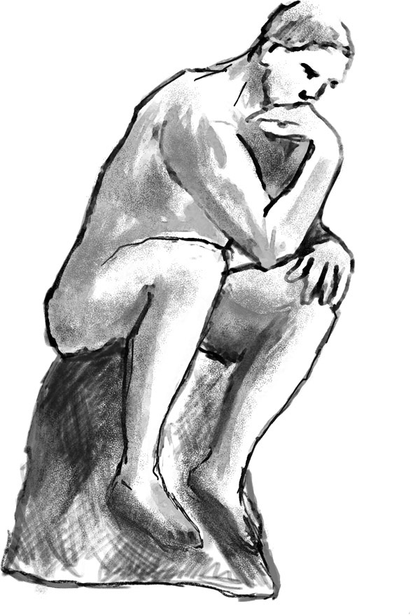
Figure 3.35 Rodin’s The Thinker sketch
In order to move joints via inverse kinematics, you first need to create a special handle to enable it. The default is the IK Handle Tool. You choose between which joints the IK handle will be created and connected. An end effector node (the driver node of the IK chain) will be created and sit on the last joint you selected, and the motion will be controlled through the IK handle via translation. The effect on the joint chain will differ depending on the type of IK solver you choose.
Some prefer IKs since they are easier to pose, but the interpolation between each key set on an IK handle is linear. You lose the arcing motion of the FK chain, since you are now translating the IK handle from one point to another in a straight line. To give the illusion of an arc, multiple keys will have to be set in an arcing shape.
As for keeping joints in their place, this is where IK handles shine. The IK handle can be locked in place through a constraint to a control object, and the root of the chain will move in relation to that locked point.
NOTE: Depending on your 3D software package of choice, the equivalent to Maya’s IK-Handles might be approached differently. Read the documentation that came with your 3D software in order to get comparable results.
There are a couple more types of useful IK solvers available. For example, the IK Spline Tool allows you to move a chain of joints by modifying the CVs of a NURBS curve. Another useful but somewhat hidden IK solver is the Spring Solver. This IK solver helps when rigging creatures or objects with multiple joints like insects or reversed-kneed creatures (usually found in demonic lore and such, or mistakenly assumed by mammals such as cats, dogs and horses that walk on the equivalent of the ball of our foot). To enable the IK Spring Solver in the IK Handle Settings menu, type the following command:
It will now appear in the dropdown for types of available IK’s with the IKHandleTool.
Attaching Meshes to Joints
Joints, on their own, won’t do much for your creatures and rigged objects. They have to be connected to the mesh in some form for them to be effective. There a few ways of achieving this, some of which we’ve already discussed above:
- Parenting—parenting the mesh to the joints is probably the quickest way of checking if the underlying skeleton works as planned. This method works great with non-organic objects made up of multiple pieces. They should ideally be grouped together in a logical construction and then parented to the relevant joint. For organic characters, usually low-resolution, proxy characters will be created—having the exact same dimensions and volume as their final high-resolution equivalent—and segmented around the main joint points. With this method, layout artists and animators can start blocking out the shots, while the final mesh and rig gets updated. The main drawback is that there isn’t any mesh deformation, so keep that in mind.
- Constraints—similar to the parenting method described above, but this time the mesh is constrained to the joints, keeping the hierarchies separated from each other. Takes a bit longer to setup, but you can use some of the more advanced constraint tools for additional control.
- Skinning—Skinning is the process of attaching a mesh to a skeleton. It is probably the most common type of mesh deformation with the use of joints, since it offers the most amount of flexibility—pun intended. The setup is more time consuming and complex than the other methods, but the end results will be as detailed as you make them.
There are two types of skinning available in Maya: Direct skinning and indirect skinning. With direct skinning, the mesh is bound directly on the joint. With indirect skinning, a deformer such as a lattice or a wrap deformer gets bound to the joint, and in turn they affect the underlying mesh.
In the case of direct skinning, the vertices on the mesh get weighted to the joints around them. Each binding type affects how the mesh will react to the joint deformations as well as how they are manipulated once bound.
NOTE: As of Maya 2015, the rigid binding option has been removed. It can still be accessed, although only through scripting. To emulate a rigid type of binding on your meshes using smooth binding, make sure the Maximum Influence is set to 1.
If you’re using a previous version of Maya, the rigid binding section will still be relevant. Keep in mind also that game engines do not do well with rigid binding, so your best option is to stick to smooth binding and paint the weights. Binding will be discussed in greater detail in Chapter 6.
In figure 3.36 you will see two polygon cylinders in a scene, both bound to an identical joint structure, but one is a smooth bind, while the second is a rigid bind. Both meshes were bound with the default smooth and rigid bind settings. Select the middle joint of each chain and rotate 35 degrees on the Y-axis of each.

Figure 3.36 Rigid and smooth bind cylinders
You’ll see that the smooth-bound cylinder bends and deforms the mesh in an almost organic, rubber-like way. On the other hand, the rigid bound cylinder has a much harsher bend, and part of the geometry actually begins to intersect itself.
Smooth Binding
The smooth bind method allows the mesh to be influenced by several joints. The influence area can be painted on interactively using the Paint Skin Weights Tool (Skin > Edit Smooth Skin > Paint Skin Weights Too l> □) or by using the Component Editor (Window > General Editors > Component Editor).
To smooth bind a mesh to a skeleton, select the skeleton chain followed by the mesh you want to bind and select Skin > Bind Skin > Smooth Bind > □ (see figure 3.37). The Smooth Bind Options window will open up and offer a variety of options to affect how the joints will affect and influence your selected mesh. You can read a detailed explanation of each of the options in Maya’s help menu.

Figure 3.37 Smooth bind options
In figure 3.38 (using Maya 2014 for this example) you can visually see the influence of the joints on the cylinder’s vertices by enabling the Paint Skin Weights Tool. Older versions of Maya were limited to showing this information only in a greyscale ramp, but now you have the option to see it as a color ramp. It’s a matter of personal preference and does not affect the functionality of the tool. To see the falloff skin weight colors, make sure that color ramp is checked under the Gradient rollout. Using the default settings, we can see that the hotter the color, the higher the influence of the joint on the vertices. As the colors begin to cool, the influence diminishes, until it there’s no effect anymore. There is an option that takes any vertices with small weight values and normalizes them fully to the joint. These small weights, for the most part, have an insignificant effect on the mesh deformation. On the other hand, they can slow down the skin processing. You can prune them to speed up the processing time and keep the weights more even. This tool is found under Skin > Edit Smooth Skin > Prune Small Weights > □. You can change the prune value according to each specific situation. Prunes are also good for low-fiber diets.
The Paint Skin Weights Tool uses Maya’s Artisan interface, so if you have a pressure-sensitive tablet, you can have finer control over weight painting. You can also set all the selected vertices in an object to 100% to a specific joint, which will prevent from blending influences, making it look like a rigid bind. Speaking of…

Figure 3.38 Smooth weight paint tool with a colored ramp
Rigid Binding
As mentioned earlier, if you’re using a version prior to Maya 2015, you can still use the rigid binding option from the menu. As opposed to its smooth counterpart, this method limits mesh points to be influenced by only one joint at a time. The most common way of editing the rigid weights is through the use of the Component Editor (Window > General Editors > Component Editor). You select vertices or CVs on your mesh, and, with the Component Editor open, you select the Rigid Skins tab. Each one of the vertices/CVs selected will have a weight value beside it, under the column representing the joint cluster it’s connected to.
Another way to change the influence of an area of a rigid bind is through the use of flexors, found under Skin > Edit Rigid Skin > Create Flexor. Flexors are deformers that allow finer control over the vertices and CVs. Some of those deformers are based on lattices, while others are sculpt and cluster deformers.
There is a way to also paint weights on a rigid bound mesh. Select Edit Deformers > Paint Cluster Weights Tool > □. It follows a similar setup as the smooth bind painting, but you don’t have the joint hierarchy present like the smooth bind. Instead, under the Paint Attributes rollout, select the joint you wish to influence by clicking the jointCluster.weights button (see figure 3.39).

Figure 3.39 Rigid bind paint attributes tool
Introduction to Scripting
Up until this point we’ve discussed some of the main rigging concepts necessary to put a rig together. There are a few more which we will cover as we proceed, including driven keys and expressions. Right now, I would like to focus on both parts of our wonderful brains and get into the truly technical aspects of rigging—scripting!
The mere mention of scripting or writing any type of code tends usually to invoke some kind of instinctive primal feelings of revulsion and fear in many an artist. It’s almost anathema to the creative spirit. Yes, scripting can be a daunting, intimidating and frustrating experience. But if understood properly, it can be a formidable tool in the creative arsenal of 3D creation. Rigging is but one aspect of it, and once harnessed, scripting can be used along any segment of the production pipeline.
Scripting can be divided into two main sections. The first is to automate and speed up repetitive tasks. Any action that has to be done time and again can, in most cases, can be scripted. The second part of scripting is to write custom tools that will help production, and enhance the default functionality of the 3D toolset.
The scripting process can be as simple as writing a single command in the Command Line or be as complex as running a full suite of scripts referencing each other and running off a remote server. The limits fall only within what you decide you want your scripts to do.
Scripting in Maya
Maya currently offers two methods of writing scripts: The original Maya Embedded Language (MEL) scripting language, as well as the more recent introduction of Python (since version 8.5).
MEL is fully integrated with Maya in the sense that any action you do within the program will trigger a MEL function representing that action. It might call a direct MEL command such as creating a polygon cube (polyCube;) or call an existing MEL script to extrude a polygonal face on that polygon cube (performPolyExtrude 0;). Maya’s user interface is an amalgamation of MEL scripts working together, executing and updating the actions done within the program. One of the biggest strengths of MEL is that most commands implemented within Maya will be echoed in the Script Editor. This offers a glimpse into the inner workings of Maya and can increase your understanding of MEL scripting as you gain experience with the language.
Another one of the advantages of MEL is that it offers a wide legacy of scripts that have been written since Maya first came out. You can find online an enormous amount of MEL scripts which you can dissect and learn from (www.creativecrash.com is a great resource for MEL scripts). As well, you can go into your Maya installation folder and look at the scripts directory. In there, you will find the core scripts that run the Maya interface and see what went into making the various tools and options offered in the program.
WARNING : make sure you copy those MEL scripts or folders first in a separate location before you start mucking around with them. You don’t want to break Maya.
Once you familiarize yourself with the workings of MEL, it is a relatively simple scripting language to pick up and work with. It uses a similar syntax to the C-language family, meaning ending code lines with a semi-colon, curly brackets to define procedures and identifying variables with the $ sign in front of them.
Python, while relatively a newcomer to Maya, has been around for years and has an extended and loyal community supporting it. A very important distinction to be aware of is that while MEL is uniquely tied to work only with Maya, Python can be used completely as a standalone language. Because of Python’s flexibility, support and adoption in the VFX industry, it has become one of the main scripting languages that connect studio pipelines between multiple software packages.
Python does have a few advantages over MEL as a scripting language, including that it:
- Is object-oriented as compared to MEL’s procedural scripting style
- Has an extended set of data-types compared to MEL’s limited one
- Has access to Maya’s Application Programming Interface (API) for deeper integration with Maya’s core engine
- Has large and comprehensive standard and user-created libraries of pre-built code and references that can greatly improve its functionality
- Has great control over data types, especially arrays, lists, dictionaries
- Has “clean” visual formatting (although some people might see this as a disadvantage due to its rigidity)
Now, unlike MEL, you cannot simply call Maya commands directly into a Python editor and expect them to work. You first have to import the correct modules prior to coding in order to have access to them. Python is effectively a wrapper around MEL, allowing the use of the Python scripting power but still following the command-based approach of MEL. In other words, think of a MEL in disguise—albeit with a faster, stronger and more flexible disguise.
There is also an additional way to script for Maya through Python, which is getting more and more exposure with each version of Maya. It is called PyMEL. PyMEL combines the power of Python but is organized in a more intuitive and clearer manner. It has obvious advantages such as brevity of code and clarity. As MEL, though, it is specific only to Maya. It is well worth exploring, though.
Options, options … it’s wonderful! In the next few sections we will discuss both scripting languages in more depth and talk more about their advantages and limitations. We will also discuss how they build on each other to offer an unprecedented amount of control over Maya. Admittedly, more and more TDs and technical artists are choosing the Python way because of its power, but knowing and understanding how MEL works will allow you to take full advantage of Maya’s capabilities and understand it better. Personally, I would take the time to familiarize myself with both flavors of Maya’s scripting languages in order to have the ability to choose when to use one or the other, depending on the needs and circumstances called for in the production.
MEL
Scripting with MEL would probably be the easiest and most straightforward way to start taking advantage of Maya’s power. Let’s start with the basics and see where that takes us.
As mentioned earlier, most of the commands executed in Maya will be echoed in the Script Editor (Window > General Editors > Script Editor). Open the Script Editor, and then create a default polygon cube. You will see the following command appear in the history panel:
In the viewport, translate the cube on the X-axis 6 units, and then rotate it on the Y-axis 30 degrees. You’ll see a sequence of commands appearing, including the following two lines:
The first action ran the command to create the cube. The second sets of commands reflect the transformations on the cube to their new position. Let’s take a look at the way these commands are constructed. This will also help us later when we analyze the Python angle of things.
Looking at the polyCube command, we see that it is made up of the command itself, which tells Maya to create our polygon cube in the viewports, followed by a sequence of flags that set specific parameters on the command and ending with a semicolon. The flags in MEL are preceded by a dash and are typically echoed with their short form version. For example, the flag w stands for width, h for height, etc. Sometimes flags will have arguments following them, setting values or conditions. Another important aspect of the MEL syntax is that commands or flags that are made up of multiple words are camel-cased, meaning they always start with a small letter, and each subsequent word has its first letter capitalized. For example: polyCube, reflectionAboutOrigin, polySphericalProjection.
You will find a list of all commands and their corresponding flags in Maya’s Help under Help > MEL Command Reference. It’s a searchable, very comprehensive and detailed help system—so do make sure to make use of it when you’re unsure about the inner workings of a specific command. A very useful feature in the help system is the list of scripting examples related to the command in question, found at the bottom of each page.
The Script Editor
Maya’s Script Editor is a good place to start delving into the arcane arts of script writing. It is divided into two sections. On top, we have the history panel that updates the actions taken by Maya as commands are processed and executed. At the bottom we have the input panel, which is where code can be entered. There are two tabs in the input panel, one for MEL scripts and the other for Python. Needless to say, make sure the correct code type you enter is in the proper tab, otherwise it won’t work.
Let’s start by customizing the Script Editor to get the most out of it. Tear off the Command menu and add a check on the following options (see figure 3.40):
- Show line numbers
- Auto-close braces
- Command Completion
- Show Tooltip Help
The first two options are self-explanatory. Line numbering greatly helps with keeping track of where actions are occurring in our script and with debugging errors. Closing braces can prevent the annoyances of having your script not executing properly because of a forgotten bracket somewhere … something we are all guilty of doing at some point or another. The last two items are optional, but if you’re starting out with MEL, it’s a good way to see the commands and flags available as you type them. You can turn off those two options once you feel comfortable with the coding process and are more familiar with the different flags and arguments.
There are a few ways to execute commands via the Script Editor. In the input area, type the following:
If you press the “Enter” key on the keyboard, your cursor will move one line down. Bring up the cursor to the end of the line you just typed and now press “Enter” on your numeric keypad. Two things will happen. The first is that the command you entered disappeared, and the second is that a flat polygonal cylinder got created in the viewport.
The command worked, but the line of code we entered is now a distant memory—at least until you press undo and bring it back to life again. Do so now, and delete the cylinder from the viewport and in the input area to bring the code back. To run the code and keep it in the Script Editor, you can do one of two things:
- Highlight the code, and press “Enter” from the numeric keypad (or CTRL-Enter).
- Press the Execute All icon (double arrows) (see figure 3.41).

Figure 3.40 Options on script editor
If you want to get help about specific commands, you can highlight the command, RMB and select Quick Help from the dropdown menu. The Quick Help window will open up on the right of the input area and show all of the flags and arguments available for that specific command. Double-clicking those flags will add them to the command line, including the arguments needed to be populated.
NOTE: The Quick Help, for the time being, shows commands and flags in MEL syntax only.

Figure 3.41 Highlighted code and Execute All button
MEL 101
Commands can be used on their own, but can also be attached to variables. Variables are like containers that hold information and can be called within the script. In MEL, variables are identified by different data types, as illustrated below:
- Integers—whole numbers, both positive and negative, without any decimals (i.e., 1,2,-738, 43, -64, etc.)
- Floats—numbers with decimal points (i.e., 4.56, 1.00, -78.904, etc.)
- Strings—alphanumeric characters (i.e., “The meaning of life is 42”)
- Vectors—a combination of 3 floating point values (i.e., <<1.618, 3.14, 9.8>>)
In MEL, variables are preceded by a $-sign. In order to define a variable, it must be first declared. For example, to declare an integer variable:
To store information in the variable, we’ll use the = (equal) sign to assign it:
For string variables, the value is placed between two sets of quotes:
If you highlight and run the line above, this is what Maya will output in the history window:
This tells us that the variable has been acknowledged, so to speak. To actually send back feedback and help in debugging our scripts, MEL offers a very useful command called the print command.
Enter this command in the line beneath $wonderland:
The result will be the value of the string. The print command is great for debugging scripts, where you can have it keep track of the actions taking place as the script is being executed.
Integer, float and string variables contain only one value per variable. In programming languages, there is a special type of variable that can hold multiple values, called an array. Arrays are defined by square brackets following the variable name.
As opposed to Python, MEL arrays can hold only values of the same data type. To populate arrays in MEL, you encompass the values in curly brackets:
Arrays are based on an index-0 system, meaning that the first value in the array has an index of 0, the second has an index of 1, the third an index of 2 and so on. For example, if you want to call out the “Moon” value, you would type the following:
The result will show:
Notice that the values in the print statement were encompassed by parentheses, and the textual element was added to the array variable with a + (plus) symbol. You’ll see more examples of this throughout the book.
Arrays don’t have to be populated with values from the beginning. They can be left as empty arrays and values added to them later on. These are called dynamic arrays. The next example will put this concept in practice, as well as introduce one of the most useful commands in Maya: ls.
ls stands for “list”. Depending on the flags enabled when running the command, it will return the names and/or name types of objects in the scene.
Create a new scene and duplicate a handful of polyCubes in it. Select them with your cursor, and type the following in the Script Editor:
First, notice the backticks ‘ ‘ surrounding the ls command. You can find them to the left of the 1-key on your keyboard, along with the ~ (tilde) key. Anytime a command is put between backticks, it tells Maya to execute that command and return the action to the variable it is paired to. In our example, this command will list the objects you selected in the viewport (the DAG nodes—remember those?), and place them in the $selObj array. One thing to remember is that they will be listed in the order you’ve selected them. The list of flags this command has is quite comprehensive and you can filter through a wide variety of selections.
As you start scripting, either for yourself or for a team-based production, it’s always good practice to comment your scripts in order to clarify and explain what went into them. Below, you’ll find a couple of ways of commenting your MEL scripts:

Anatomy of a Script
One of the staples of scripting is the ability to loop the code to affect a sequence of objects or variables. Let’s say that you want to turn all selected objects into wireframes while the viewport is still in shaded mode, and prevent them from being rendered at render time. To make things a bit more interesting, let’s assume that there is a child node attached to our main selected objects. In figure 3.42, you’ll see 4 cubes, with spheres in each one of them parented to the cubes. The view is in X-ray mode so you can see through for your convenience, and so you can validate the veracity of said statement.
In the next example we will go step-by-step and detail the breakdown of a simple script.

Next, we start the loop. We will use a for-loop which is a specialized loop geared to work with array iterations. The format is: for (element in array) {repeatable action;} . The element variable does not have to be pre-defined.

Before we get into the details of the for-loop, there’s one thing to remember for this exercise: the visibility attribute affects the Transform node of the object. So in this case, if we were to hide the visibility attribute, it would also affect the child nodes, turning them into wireframes as well. We want to affect only the Shape node of the object, while leaving the child nodes as they are. For this, we will need to drill down the Transform node and use the listRelatives command to get to the Shape node. Here’s what we should have so far:

The reason we use $shapeObj[0] is that in this case, the element in the for-loop iterates only one object at a time. And since our indices are 0-based, it is the first and only number in the loop.
The next command we will add to our script is the setAttr command. It stands for “set attribute” and allows us to change an attribute on the object in question. In this case, we will first override the Drawing Overrides option and, second, turn off the shading option. And, while we’re at it, we’ll also turn off the Primary Visibility of the cubes so they don’t render. The zeroes and ones at the end of the setAttr lines, in this particular case, stand for “off” and “on”. You can use this script to create polygonal control characters for your rigs (see figure 3.43).

There are other types of for-loops, but we will discuss them as needed. All these loop types will make an appearance again as we discuss Python scripting in-depth a bit further in the book.
The true power of scripting comes from combining commands into contained functions. In MEL these functions are called procedures. Simple scripts can run with no defined procedures—especially if they’re being run directly from the Script Editor or as a custom button from the shelf tabs. Yet, if you want to define a script, save it and re-use it in Maya, you will need to start defining procedures to call and execute the code in them.

Figure 3.43 End result of for-loop overriding the visibility of the cubes (shown as wireframe)
Think of each procedure as a cog in a machine, with each cog in charge of certain behaviors or calculations. When combined together, these cogs execute their dedicated function and make the machine run smoothly and effectively. You can define in your script, for example, a procedure that will create the GUI and user interaction, a procedure for error checks, and specific procedures for each type of calculation you want Maya to run on your objects.
There are two types of available procedures: local and global. Local procedures are the default, and they are declared as follows:

The difference between local and global procedures is that local procedures can be called only within the scope of the script in which they were created. Global procedures, on the other hand, can be called and made available from anywhere. As an example, you can have a library of custom scripts, where scriptA.mel calls on a global procedure defined by scriptE.mel. You can combine global and local procedures within a MEL script, depending on the functionality you are looking to achieve. To make a script global, simply type the word global in front of proc.
NOTE: A local procedure cannot be declared in the Script Editor. Instead, it has to be specified in an external script file. In other words, every procedure and variable created and executed in the Script Editor becomes global and remains accessible in memory, until you shut Maya down.
Here’s a very basic procedure used to create a simple polygon cube:

Highlight the procedure, and press CTRL-Enter. The procedure is now in memory. If you type cubeMaker in the command line (make sure it’s set to MEL), you’ll see a cube show up in the viewport, going by the name of “myCube”. Run the procedure again, another cube—this time with the number 1 appended to its name—will show up. You can repeat that command as many times as you want, and a new “myCube” will appear, each uniquely identified by the number attached to its name. Yawn! Ok, let’s make this a bit more interesting. Let’s say we want to specify how many cubes we want to create, and then translate and rotate those cubes based on their creation sequence, and throw some other fun stuff in there:

Execute the script (pay attention to the backticks around the cos and sin commands!) and enter the following in the MEL command line: cubix 100.
Guess what? I don’t think we’re in Kansas anymore (see figure 3.44)!

Figure 3.44 Cubix tornado created through the script
Procedures can also return statements. Place the type of variable you want to be returned before the procedure name. Here’s a basic example:

Run the procedure, this time putting your first and last name after myName as follows:
The return statement will display the data you entered within the sentence.
NOTE: the after the period is called an escaped character. When certain characters are placed after a backslash, Maya interprets them in a different way. For example, in our case, it means newline. This means that once the line is printed, it will go down to a new line.
Some other escaped characters:
carriage return
tab
” prints double quotes
\ prints a backslash
Saving the Script
As with most things in Maya, there are multiple ways of running your scripts. The first is to save the script on a shelf. In the Script Editor, highlight your script, then MMB-drag the highlighted code to the shelf. Maya should be able to identify the script language automatically. If not, you’ll be prompted to save it either as MEL or Python. The one disadvantage of this method is that you are copying the full script into the shelf button, and it might make it awkward to edit and debug.
A better way is to save your scripts as individual files. The most straightforward way is to highlight your code in the Script Editor, go to File > Save Script… Maya will prompt you where you want to save your script, with the default .mel extension. There are 3 “scripts” folders available for you to save your scripts into, all under the <Users<name>Documentsmaya> directory (in Windows). I personally save it under the “prefs” folder, but you can use any of the three. For me, saving it in that location means that I can back that folder up and zip it or email it so I can keep all of my custom scripts, icons and shelves all under one directory.
NOTE: For Mac or Linux, check for the relevant location of those folders in the documentation.
It is customary to save your script with the name of your main procedure. Looking at the cubix example a couple of pages back, you can save the file as cubix.mel. It is also recommended to make the procedure global before saving it, so it can be accessed at any time, otherwise you might get a “Cannot find procedure “<name>” error. Another common practice is to put your initials in front of your procedures. With the amount of scripts available out there, you never know if someone might have used the same naming convention as you did. By using your initials, you reduce the chance of name conflict from happening.
For example, this would be the final version of the cubix script, set as a global procedure:

In this case, I would save it as eaCubix.mel.
As a quick aside, writing short scripts in the Script Editor might be sufficient, but if you are planning on doing heavy-duty script writing, seriously consider using a fully featured text editor or a dedicated Integrated Development Environment (IDE). As I mentioned in the introduction, I use Eclipse as my main scripting environment—especially with Python.
Once your MEL script is saved, there are a few steps you must first do before it is ready to be run:
-
Rehash—when saving a script while Maya is open and running, you must first refresh and update Maya’s list of existing scripts. To do so, type the
rehashcommand in the command line. Closing and opening Maya will automatically update the script list, but it’s a counter-intuitive method. -
Source—if you decide to change the content of your script after you’ve saved it, Maya won’t update it automatically. You have to use the
sourcecommand to do that. The format issource <filename>.mel.
We talked briefly earlier about dragging and dropping your script to the shelf as a button, and the potential disadvantage of saving a long script as such. An efficient method, instead, would be to save the script as a .mel file and create a shelf button with the source command and the procedure name. Using our previous script as an example:
This way, if you ever need to make additional changes to the script, it will run with the updated changes.
This was but a tiny fraction of what can be accomplished with MEL scripting. In the following sections and chapters we will expand our scripting scope using Python, with the occasional MEL command thrown in for flavor or simple convenience, as needed.
Python
I found that one of the best ways to learn a tool or related concept is to jump right in and immerse myself in it. In this next section, we will create the first production script for the Tin game. This script will allow us to easily create gears and cogs (a must in anything vaguely mechanical). Although it is not a rigging script per se, this will introduce some of the basic concepts of scripting with Python.
NOTE: One extremely important point to mention … Python is an indent-based language, so the indentation order is critical, otherwise it will throw errors back. Due to the layout and formatting of this book, some of the code will wrap across the margins and will look wrong, especially with Python. The code shown here is only for example purposes. Please go to the companion website at www.thetingirl.com and download the properly formatted code for review.
If you see a set of triple arrows at the end of a line of code (i.e., >>>), it means the code actually continues on that same line.
Python, like MEL, can be used as a procedural language. This means that it can run a sequence of contained subroutines or functions, each running a specific action in a top-down sequence. On the other hand, the strength of Python can be truly leveraged when used as an object-oriented programming (OOP) language, thus allowing the creation of modular objects that can be used and reused throughout the script(s). We will explore OOP further along in upcoming chapters. For now, in this first script, we will transition gently into Python using the procedural approach. This will offer a good introduction to the language as well as help transition those of you who do have previous MEL experience, to see and compare the language differences and approaches. The key right now is to note the syntax differences in the way Python calls the Maya commands and their respective flags.
In order for Maya to recognize the Python scripts, there are a couple of small things to enable in the interface. First, in the command line, click on the word “MEL” to change it to “Python” (see figure 3.45). Now Maya will know that you are entering Python commands. Just make sure to switch back if you go back to MEL at any point.
Figure 3.45 MEL/Python command line
Next, in the Script Editor, you’ll notice the two types of tabs above the input area. Obviously, the Python one is the one we want. To create additional tabs, RMB-click in the input area, select “New tab…” from the radial menu and then choose the scripting language you wish to code in.
Unlike in MEL, where the core Maya commands are built in the scripting language—in Python they have to be explicitly imported. We will use the import command to do so:
This action will load Maya’s core commands module and allow us similar access as we would have in MEL. For example, to create a simple polygon cube, we will type:
The one drawback in this method is that you’ll have to prefix every Maya command with maya.cmds in front of it. Not too worry; there is a more elegant way to do so using an alias:
In this way, we will be using mc as an alias for maya.cmds.
NOTE:
You can use any alias you want, but it’s recommended to stick with some of the standards to prevent confusion in case you wish to share your scripts. Another typical alias used when importing Maya commands is “cmds” (which you will find in Autodesk’s documentation). Another method is to do completely away with aliases and use:
from maya.cmds import *
This will bring all of Maya commands into the top-level namespace and there is no need to prefix it with anything. The possible drawback is that there might be a slight chance of conflict between Maya commands and Python commands. Caveat emptor! I personally prefer to use “mc”.
Now, to create our polygon cube with the mc alias, this time we will simply type:
NOTE: In Python, every Maya command is followed by a set of parentheses. Empty parentheses are the default command, while the command’s flags will be within those parentheses. And just to reiterate one more time: Indentation is very important when scripting with Python.
Our First Python Script—tgpGears
Fire up your IDE of choice and type the following lines:

We will be importing commands from the random module, which we will make use of further down in our script. This is one of the ways Python stays trim and light, by allowing users to bring in only the commands they need, rather than loading into memory everything including the proverbial kitchen sink.
As well, we will import the partial command from a Python module called functools. According to the Python documentation, functools allows “for higher-order functions: functions that act on or return other functions”. For our purposes, the partial() function in this module will offer the ability to pass additional arguments to a callback function, for example when calling a function triggered by a radio button.
Navigate to your Maya scripts directory and save the file as tgpGears.py. In the next lines, we will create our first function. Functions in Python are the equivalent of procedures in MEL. I usually tend to create the first function with the name of the script and use it as a kind of gateway for other functions in case I need to check for necessary plugins, references, load UI’s, etc.
NOTE:
In Python, comments are preceded by the # (hash) symbol. To comment a block of lines, you can either use three ‘’’ (single) or “”” (double) quotes before and after the commented block.

The def command defines the name of the Python function. In this particular case, our function will print the statement in the Script Editor and run the tgpGearUI function, where we will create the user interface for our gear maker script.
Creating the GUI
For the interface we will use Maya’s ELF (Extension Layer Framework) commands. These are special commands that allow the creation of custom interface elements.
NOTE: An alternate method of creating interfaces in Maya with Python is by using the QT Designer application. It offers a WYSIWYG layout, rather than coding the GUI elements. We won’t cover its use in this book, but feel free to read the documentation and try your hand designing GUIs with it.
This is the basic frame of our interface:


When creating UI widget elements, Maya passes on automatically an additional number of arguments to the function. The *args argument inside the tgpGearsUI() function acts as a general catch-all for those unspecified number of arguments. This will help us prevent argument-related errors in the future.
We first have to check if the window already exists and if it is open in the viewports. Without this check, Maya would have thrown an error stating that the window is not unique. To prevent this from happening, we check if our window exists. If it does, then we run the deleteUI command to remove it. We will also check for the window preferred attributes such as size and position, and remove them in order to reset the window to its default size.
Next is where we create the actual UI window. The various flags and their descriptions can be found under Maya’s Help > Python Command Reference. Use the search bar for the specific command you’re looking for. Finally, we display the window using the showWindow command. Remember to save your file!
As opposed to MEL, we don’t have rehash or source commands in Python. Instead, we will load our script by opening the Script editor and typing the following lines in a Python tab:

We first import our script into Python. The reload command is there to refresh the script, if you will. It’s similar in action to the MEL source command in the sense that if you update the code, it will always load the latest version of the script, rather than what was originally loaded into memory the first time it was executed. The last line tells Python which function from the script to load. Highlight the code and execute it. You should see an empty UI window floating above the viewports (see figure 3.46).
NOTE: You might want to make a shelf button from those lines for convenience. After you highlight them, MMB-drag and drop those lines on one of your Maya shelves. You can now simply click on that button to run the script.

Figure 3.46 Empty UI window
Our next feature will be to create a drop-down menu that will reset our UI to its defaults. Go back to the script and type the following after the mc.window(…) command:

The “Edit” option will appear under our window title. When clicked, the “Reset” command will be offered. Executing it will call the tgpGearsUI() function, in effect reloading the script.
The next few lines will complete the creation of the UI elements of our script. They will focus on creating the various buttons, sliders, and input fields in our gears script. The commands are self-explanatory for the most part, calling for the various interface controls, their position within the UI framework, and any default values they might start with, and calling additional functions via commands. In the case of tgpCheckType, this is where the Python partial command comes into play, allowing for calling another function and passing a condition argument to it. We’ll discuss that further down.
One thing to note—make sure to give each and every one of the interface commands a unique name! This will greatly help with querying the controls, getting information from them or piping information back. For the sake of brevity, the shortened versions of the flags have been used in most instances (i.e., v instead of value). Below is the full tgpGearsUI() function.


If we try running the script right now, we will encounter an error, stating the following:

Our script is looking for functions that we have not created yet (tgpChangeType, tgpUserGear, tgpRandomGear). When it doesn’t find them within the code, it throws back those errors to let us know.
Let’s fix that by creating those functions now. Enter them below the block of code we entered earlier and use the pass command in the body of each of the functions. The pass command creates a null operation—in other words, it doesn’t do anything—and works great as a placeholder for future code that will go in the function.

Now, if we run the script again, we will see our UI in all of its UI-like glory (see figure 3.47).

Figure 3.47 Populated UI window
Querying the GUI Values
Great! Now it’s time to get those gears in working order. Our next function will check if we are creating a hollow or a solid gear. If the user selects Hollow, the Gear inner radius option will be available for modification. If Solid is selected, it will be greyed out. This process is actually related to one of the key components of good scripting, which is checking for potential user errors. The last thing you want your script to do is crash because of an unanticipated user function.
As mentioned above, the tgpChangeType function was called via the partial command. In it, the variable checkBody is assigned to the radioButtonGrp command gearBody that was created in the UI function. The main difference now is that instead of creating the UI buttons, it actually is querying (using the q, or query flag) which of the buttons was selected.
If the query of checkBody returns our first selection (hollow gear), then the UI stays unchanged and accessible to the user. This is done by setting the enable flag to true. On the other hand, if the second option (solid gear) is selected, then the option is greyed out. In this case, enable is set to false. The else command works well in a situation where a true/false condition exists. For multiple options, you can use the elif command (else-if).

The role of the next function in our script is to query all of the values from the UI and attach them to variables. Those values will then be passed to a function that will determine the type of gear that will be created and apply the relevant calculations to it.
The key aspect of this function is to pass those variables as arguments to the next function in our script, as seen in the last line of the following segment.

NOTE: I’ve prefixed the variable names with a g (for gear). It’s just a habit of mine to keep continuity—and uniqueness—within the script. You’ll find that as you develop your own coding practices, you’ll come up with your own ways of doing things.
Remember when we started our script, we imported the random module? The next section will make use of it in order to generate random values, instead of the user entered values. The first step will be to populate each variable with a random value—including the minimum and maximum ranges of each value. Once each variable is defined, we will provide a visual feedback to the user and update the UI with the generated values. This way, in case the user likes the end result that was randomly created, they will be able to recreate or tweak it to their taste.
To update the UI fields, the edit (or its short form “e”) flag is used to change the pre-existing values.


The previous couple of functions were similar in scope, both passing the gear values to the next function block, but each obtaining that information from different sources.
Creating the Gears
With the gear values firmly in place, the next phase of the script will focus on creating the 3D geometry of the gear.

The first part of this particular function deals with the creation of a set in which we will place all of our script-generated gears. If the set already exists in the scene, the user is notified. Otherwise, a new set is created using the text field entry. Sets are a wonderful way of keeping your scenes all neat and tidy, and offer some additional functionality in terms of selections and setups.
The next section code section sets a variable to check the axis in which the gear will be created. The UI radio buttons get queried, and a new function—tgpGetAxis—gets called with that variable as an argument.
The rest of the function checks if the gear selection was a hollow or solid. Based on that information, the formula sets the start and end faces of the geometry to extrude the gear teeth from and passes it to the relevant function to generate the gear model itself.
Let’s analyze the next bit of code. Until now, especially if you are familiar with MEL, you might have noticed that so far the majority of the commands in the script were very similar to MEL’s own structure—apart from the obvious difference of Python’s syntax. The tgpGetAxis function in the next segment will introduce us to a Python feature called dictionaries.
A dictionary in Python acts as a container that—unlike other lists which hold sequences of single items—holds paired items. The first item is the key to the second item’s value.
Before detailing the workings of our particular dictionary in this script, we have to figure out what Maya does when a polygonal object is created and its axis of creation is modified from the defaults. Create a polygon cylinder, and from the options, change the axis from the default Y-axis to the Z-axis.
If you check the Script Editor, you’ll see the following line:
The detail we’re looking for is the—ax flag. Notice that it has three values that follow it, one for each orthographic axis. In this case, both the X- and Y-axes have a value of zero, while the Z-axis has a value of 1.
If you recall also when we created the UI, the gearAxis radioButtonGrp had 3 label values—“X”, “Y”,”Z”. Each one of those labels has an index number attached to them, ranging between 1 and 3. For our example, we need to pipe in the correct 3 values into our axis flag when the gear geometry gets created. In cases like these, dictionaries really shine and make scripting very straightforward and clean.
As mentioned earlier, in the previous function, we queried the value of gearAxis and passed that on as an argument when we call the current tgpGetAxis function. The argument should give us a value between 1 and 3 depending on the selection.
We then create a variable that defines the keys in our dictionary. Key 1, which corresponds to the X-axis, will have a value of 1, 0, 0. Following this setup, we apply the second and third keys in the dictionary.
Lastly, we create a set of if statements that match the selected axis to their proper values, and that information is sent back to our previous function—tgpCheckGearType—using a return statement. Very useful, these return statements…

To complete our script, we will create the last two functions that actually build the geometry for the gears. All of the information we have collected and processed in the earlier functions will now be sufficient to tweak the primitive polygon meshes and turn them into our gear assets. Both functions work identically to each other, the difference being that tgpHollow uses a pipe primitive while tgpSolid uses a cylinder primitive.


The code is pretty straightforward. Once the flags for the primitive geometry are set and the number of gear teeth is known, a for-loop is created to select the relevant faces and extrude them out.
String Formatting in Python
The interesting—and very useful—Python functionality present in these few lines of code is the .format() method.
String formatting allows us to do complex variable and value substitutions in our code. It takes a bit of getting used to if you come straight from MEL, but once you get the hang of it, it sure beats concatenating strings hands down!
Here’s a quick example of the. format() method:

The values are placed between curly {} brackets (note that they are 0-indexed) and called in sequential order from within the .format() method at the end of the string. There are many other ways to substitute the values, which are too many to cover in this Python introduction.
This method is set to replace the older way of string substitution that used the % (modulo) operator. Here’s the same example as above using this method:
At first glance, it looks the same, if not even simpler. The % operator can be combined with a variation of suffixes to represent various argument types, i.e., %s for string, %f for floats, %d for integers, etc. You will probably encounter quite a few examples of code still using this method, but according to the good folk developing Python, it is being deprecated and the use of .format() is encouraged when writing code from Python v2.6 and up. Some of the advantages the .format() method has over the % operator include added flexibility in terms of operations and re-using of arguments.
NOTE: You can find the full documentation of Python commands at docs.python.org.
Congratulations! The script is complete and ready to be run in Maya. With this we complete the rigging overview chapter. The process of scripting touched on a few basic but important foundation concepts that will help you build more complex tools. This will aid you with the rigging—and general—pipelines found in 3D productions.