
STRUCTURE-BASED (WHITE-BOX) TECHNIQUES
Structure-based test techniques are used to explore system or component structures at several levels. At the component level, the structures of interest will be program structures such as decisions; at the integration level we may be interested in exploring the way components interact with other components (in what is usually termed a calling structure); at the system level we may be interested in how users will interact with a menu structure. All these are examples of structures and all may be tested using white-box test case design techniques. Instead of exercising a component or system to see if it functions correctly white-box tests focus on ensuring that particular elements of the structure itself are correctly exercised. For example, we can use structural testing techniques to ensure that each statement in the code of a component is executed at least once. At the component level, where structure-based testing is most commonly used, the test case design techniques involve generating test cases from code, so we need to be able to read and analyse code. As you will see later, in Chapter 6, code analysis and structure-based testing at the component level are mostly done by specialist tools, but a knowledge of the techniques is still valuable. You may wish to run simple test cases on code to ensure that it is basically sound before you begin detailed functional testing, or you may want to interpret test results from programmers to ensure that their testing adequately exercises the code.
Our starting point, then, is the code itself.
|
READING AND INTERPRETING CODE In a Foundation-level examination the term‘code‘ will always mean pseudo code. Pseudo code is a much more limited language than any real programming language but it enables designers to create all the main control structures needed by programs. It is sometimes used to document designs before they are coded into a programming language. In the next few boxes we will introduce all the essential elements of pseudo code that you will need to be able to analyse code and create test cases for the Foundation examination. Wherever you see the word ‘code‘ from here on in this chapter read it as ‘pseudo code‘. |
Real programming languages have a wide variety of forms and structures—so many that we could not adequately cover them all. The advantage of pseudo code in this respect is that it has a simple structure.
|
OVERALL PROGRAM STRUCTURE Code can be of two types, executable and non-executable. Executable code instructs the computer to take some action; non-executable code is used to prepare the computer to do its calculations but it does not involve any actions. For example, reserving space to store a calculation (this is called a declaration statement) involves no actions. In pseudo code non-executable statements will be at the beginning of the program; the start of the executable part is usually identified by BEGIN, and the end of the program by END. So we get the following structure: 1 Non-executable statements 2 BEGIN 3 4 Executable statements 5 6 END If we were counting executable statements we would count lines 2, 4 and 6. Line 1 is not counted because it is non-executable. Lines 3 and 5 are ignored because they are blank. If there are no non-executable statements there may be no BEGIN or END either, but there will always be something separating non-executable from executable statements where both are present. |
Now we have a picture of an overall program structure we can look inside the code. Surprisingly, there are only three ways that executable code can be structured, so we only have three structures to learn. The first is simple and is known as sequence: that just means that the statements are exercised one after the other as they appear on the page. The second structure is called selection: in this case the computer has to decide if a condition (known as a Boolean condition) is true or false. If it is true the computer takes one route, and if it is false the computer takes a different route. Selection structures therefore involve decisions. The third structure is called iteration: it simply involves the computer exercising a chunk of code more than once; the number of times it exercises the chunk of code depends on the value of a condition (just as in the selection case). Let us look at that a little closer.
|
PROGRAMMING STRUCTURES SEQUENCE The following program is purely sequential: 1 Read A 2 Read B 3 C = A + B The BEGIN and END have been omitted in this case since there were no non-executable statements; this is not strictly correct but is common practice, so it is wise to be aware of it and remember to check whether there are any non-executable statements when you do see BEGIN and END in a program. The computer would execute those three statements in sequence, so it would read (input) a value into A (this is just a name for a storage location), then read another value into B, and finally add them together and put the answer into C. SELECTION 1 IF P > 3 2 THEN 3 X = X + Y 4 ELSE 5 X = X − Y 6 ENDIF Here we ask the computer to evaluate the condition P > 3, which means compare the value that is in location P with 3. If the value in P is greater than 3 then the condition is true; if not, the condition is false. The computer then selects which statement to execute next. If the condition is true it will execute the part labelled THEN, so it executes line 3. Similarly if the condition is false it will execute line 5. After it has executed either line 3 or line 5 it will go to line 6, which is the end of the selection (IF THEN ELSE) structure. From there it will continue with the next line in sequence. There may not always be an ELSE part, as below: 1 IF P > 3 2 THEN 3 X = X + Y 4 ENDIF In this case the computer executes line 3 if the condition is true, or moves on to line 4 (the next line in sequence) if the condition is false. ITERATION Iteration structures are called loops. The most common loop is known as a DO WHILE (or WHILE DO) loop and is illustrated below: 1 X = 15 2 Count = 0 3 WHILE X < 20 DO 4 X = X + 1 5 Count = Count + 1 6 END DO As with the selection structures there is a decision. In this case the condition that is tested at the decision is X < 20. If the condition is true the program <enters the loop< by executing the code between DO and END DO. In this case the value of X is increased by one and the value of Count is increased by one. When this is done the program goes back to line 3 and repeats the test. If X < 20 is still true the program <enters the loop< again. This continues as long as the condition is true. If the condition is false the program goes directly to line 6 and then continues to the next sequential instruction. In the program fragment above the loop will be executed five times before the value of X reaches 20 and causes the loop to terminate. The value of Count will then be 5. There is another variation of the loop structure known as a REPEAT UNTIL loop. It looks like this: 1 X = 15 2 Count = 0 3 REPEAT 4 X = X + 1 5 Count = Count + 1 6 UNTIL X = 20 The difference from a DO WHILE loop is that the condition is at the end, so the loop will always be executed at least once. Every time the code inside the loop is executed the program checks the condition. When the condition is true the program continues with the next sequential instruction. The outcome of this REPEAT UNTIL loop will be exactly the same as the DO WHILE loop above. |
|
CHECK OF UNDERSTANDING
|
Flow charts
Now that we can read code we can go a step further and create a visual representation of the structure that is much easier to work with. The simplest visual structure to draw is the flow chart, which has only two symbols. Rectangles represent sequential statements and diamonds represent decisions. More than one sequential statement can be placed inside a single rectangle as long as there are no decisions in the sequence. Any decision is represented by a diamond, including those associated with loops.
Let us look at our earlier examples again.
To create a flow chart representation of a complete program (see Example 4.5) all we need to do is to connect together all the different bits of structure.
Figure 4.4 Flow chart for a sequential program

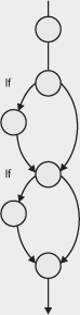
Figure 4.5 Flow chart for a selection (decision) structure

Figure 4.6 Flow chart for an iteration (loop) structure

|
PROGRAM ANALYSIS—EXAMPLE 4.5 Here is a simple program for calculating the mean and maximum of three integers. 1 Program MaxandMean 2 3 A, B, C, Maximum: Integer 4 Mean: Real 5 6 Begin 7 8 Read A 9 Read B 10 Read C 11 Mean = (A + B + C)/3 12 13 If A > B 14 Then 15 If A > C 16 Then 17 Maximum = A 18 Else 19 Maximum = C 20 Endif 21 Else 22 If B > C 23 Then 24 Maximum = B 25 Else 26 Maximum = C 27 Endif 28 Endif 29 30 Print (“Mean of A, B and C is “, Mean) 31 Print (“Maximum of A, B, C is “, Maximum) 32 33 End Note one important thing about this code: it has some non-executable statements (those before the Begin and those after the Begin that are actually blank lines) that we will have to take account of when we come to count the number of executable statements later. The line numbering makes it a little easier to do the counting. By the way, you may have noticed that the program does not recognise if two of the numbers are the same value, but simplicity is more important than sophistication at this stage. This program can be expressed as a flow chart; have a go at drawing it before you look at the solution in the text. |
Figure 4.7 shows the flow chart for Example 4.5.
Figure 4.7 Flow chart representation for Example 4.5

Before we move on to look at how we generate test cases for code, we need to look briefly at another form of graphical representation called the control flow graph.
Control flow graphs
A control flow graph provides a method of representing the decision points and the flow of control within a piece of code, so it is just like a flow chart except that it only shows decisions. A control flow graph is produced by looking only at the statements affecting the flow of control.
The graph itself is made up of two symbols: nodes and edges. A node represents any point where the flow of control can be modified (i.e. decision points), or the points where a control structure returns to the main flow (e.g. END WHILE or ENDIF). An edge is a line connecting any two nodes. The closed area contained within a collection of nodes and edges, as shown in the diagram, is known as a region.

We can draw ‘subgraphs‘ to represent individual structures. For a flow graph the representation of sequence is just a straight line, since there is no decision to cause any branching.
|
CONTROL FLOW SUBGRAPHS
|

The subgraphs show what the control flow graph would look like for the program structures we are already familiar with.
|
DRAWING A CONTROL FLOW GRAPH The steps are as follows:
|
Any chunk of code can be represented by using these subgraphs.
As an example, we will return to Example 4.5.
Step 1 breaks the code into statements and identifies the control structures, ignoring the sequential statements, in order to identify the decision points; these are highlighted below.
1 	Program MaxandMean
2
3 	A, B, C, Maximum: Integer
4 	Mean: Real
5
6 	Begin
7
8 	Read A
9 	Read B
10	Read C
11	Mean = (A + B + C)/3
12
13	If A > B
14	Then
15		If A > C
16		Then
17			Maximum = A
18		Else
19			Maximum = C
20		Endif
21	Else
22		If B > C
23		Then
24			Maximum = B
25		Else
26			Maximum = C
27		Endif
28	Endif
29
30	Print (“Mean of A, B and C is “, Mean)
31	Print (“Maximum of A, B, C is “, Maximum)
32
33	End
Step 2 adds a node for each branching or decision statement (Figure 4.8).
Step 3 expands the nodes by substituting the appropriate subgraphs (Figure 4.9).
Figure 4.8 Control flow graph showing subgraphs as nodes

Figure 4.9 Control flow graph with subgraphs expanded

|
CHECK OF UNDERSTANDING
|
Exercise 4.6
| Exercise 4.6 |
Draw a flow chart and a control flow graph to represent the following code:
1 	Program OddandEven
2
3 	A, B: Real;
4 	Odd: Integer;
5
6	Begin
7 		Read A
8 		Read B
9 		C = A + B
10		D = A − B
11		Odd = 0
12
13		If A/2 DIV 2 << 0 (DIV gives the remainder after division)
14		Then Odd = Odd + 1
15		Endif
16
17		If B/2 DIV 2 << 0
18		Then Odd = Odd + 1
19		Endif
20
21		If Odd = 1
22		Then
23			Print (“C is odd“)
24			Print (“D is odd“)
25		Else
26			Print (“C is even“)
27			Print (“D is even“)
28		Endif
29	End
The answer can be found at the end of the chapter. |
Statement testing and coverage
Statement testing is testing aimed at exercising programming statements. If we aim to test every executable statement we call this full or 100 per cent statement coverage. If we exercise half the executable statements this is 50 per cent statement coverage, and so on. Remember: we are only interested in executable statements, so we do not count non-executable statements at all when we are measuring statement coverage.
Why measure statement coverage? It is a very basic measure that testing has been (relatively) thorough. After all, a suite of tests that had not exercised all of the code would not be considered complete. Actually, achieving 100 per cent statement coverage does not tell us very much, and there are much more rigorous coverage measures that we can apply, but it provides a baseline from which we can move on to more useful coverage measures. Look at the following pseudo code:
1 	Program Coverage Example
2 	A, X: Integer
3 	Begin
4 		Read A
5 		Read X
6 		If A > 1 AND X = 2
7 		Then
8 			X = X/A
9 		Endif
10		If A = 2 OR X = 2
11		Then
12			X = X + 1
13		Endif
14	End
A flow chart can represent this, as in Figure 4.10.
Having explored flow charts and flow graphs a little, you will see that flow charts are very good at showing you where the executable statements are; they are all represented by diamonds or rectangles and where there is no rectangle there is no executable code. A flow graph is less cluttered, showing only the structural details, in particular where the program branches and rejoins. Do we need both diagrams? Well, neither has everything that we need. However, we can produce a version of the flow graph that allows us to determine statement coverage.
To do this we build a conventional control flow graph but then we add a node for every branch in which there is one or more statements. Take the Program Coverage example; we can produce its flow graph easily as shown in Figure 4.11.
Before we proceed, let us confirm what happens when a program runs. Once the program starts it will run through to the end executing every statement that it comes to in sequence. Control structures will be the only diversion from this end-to-end sequence, so we need to understand what happens with the control structures when the program runs. The best way to do that is to ‘dry run‘ the program with some inputs; this means writing down the inputs and then stepping through the program logic noting what happens at each step and what values change. When you get to the end you will know what the output values (if any) will be and you will know exactly what path the program has taken through the logic.
Figure 4.10 Flow chart for Program Coverage Example

|
PATHS THROUGH A PROGRAM Flow charts, control flow graphs and hybrid flow graphs all show essentially the same information, but sometimes one format is more helpful than another. We have identified the hybrid flow graph as a useful combination of the control flow graph and the control flow chart. To make it even more useful we can add to it labels to indicate the paths that a program can follow through the code. All we need to do is to label each edge; paths are then made up from sequences of the labels, such as abeh, which make up a path through the code (see Figure 4.12). Figure 4.12 Paths through the hybrid flow graph
|
In the Program Coverage example, for which we drew the flow chart in Figure 4.10, 100 per cent statement coverage can be achieved by writing a single test case that follows the path acdfgh (using lower case letters to label the arcs on the diagram that represent path fragments). By setting A = 2 and X = 2 at point a, every statement will be executed once. However, what if the first decision should be an OR rather than an AND? The test would not have detected the error, since the condition will be true in both cases. Similarly, if the second decision should have stated X > 2 this error would have gone undetected because the value of A guarantees that the condition is true. Also, there is a path through the program in which X goes unchanged (the path abeh). If this were an error it would also go undetected.
Remember that statement coverage takes into account only executable statements. There are 12 in the Program Coverage example if we count the BEGIN and END statements, so statement coverage would be 12/12 or 100 per cent. There are alternative ways to count executable statements: some people count the BEGIN and END statements; some count the lines containing IF, THEN and ELSE; some count none of these. It does not matter as long as:
You exclude the non-executable statements that precede BEGIN.
You ignore blank lines that have been inserted for clarity.
You are consistent about what you do or do not include in the count with respect to control structures.
As a general rule, for the reasons given above, statement coverage is too weak to be considered an adequate measure of test effectiveness.
|
STATEMENT TESTING—EXAMPLE 4.6 Here is an example of the kind you might see in an exam. Try to answer the question, but if you get stuck the answer follows immediately in the text. Here is a program. How many test cases will you need to achieve 100 per cent statement coverage and what will the test cases be? 1 Program BestInterest 2 Interest, Base Rate, Balance: Real 3 4 Begin 5 Base Rate = 0.035 6 Interest = Base Rate 7 8 Read (Balance) 9 If Balance > 1000 10 Then 11 Interest = Interest + 0.005 12 If Balance < 10000 13 Then 14 Interest = Interest + 0.005 15 Else 16 Interest = Interest + 0.010 17 Endif 18 Endif 19 20 Balance = Balance × (1 + Interest) 21 22 End |
Figure 4.13 shows what the flow graph looks like. It is drawn in the hybrid flow graph format so that you can see which branches need to be exercised for statement coverage.
Figure 4.13 Paths through the hybrid flow graph

It is clear from the flow graph that the left-hand side (Balance below £1,000) need not be exercised, but there are two alternative paths (Balance between £1,000 and £10,000 and Balance ££10,000) that need to be exercised.
So we need two test cases for 100 per cent statement coverage and Balance = £5,000, Balance = £20,000 will be suitable test cases.
Alternatively we can aim to follow the paths abcegh and abdfgh marked on the flow graph. How many test cases do we need to do that?
We can do this with one test case to set the initial balance value to a value between £1,000 and £10,000 (to follow abcegh) and one test case to set the initial balance to something higher than £10,000, say £12,000 (to follow path abdfgh).
So we need two test cases to achieve 100 per cent statement coverage in this case.
Now look at this example from the perspective of the tester actually trying to achieve statement coverage. Suppose we have set ourselves an exit criterion of 100% statement coverage by the end of component testing. If we ran a single test with an input of Balance = £10,000 we can see that that test case would take us down the path abdfgh, but it would not take us down the path abcegh, and line 14 of the pseudo code would not be exercised. So that test case has not achieved 100% statement coverage and we will need another test case to exercise line 14 by taking path abcegh. We know that Balance = £5000 would do that. We can build up a test suite in this way to achieve any desired level of statement coverage.
|
CHECK OF UNDERSTANDING
|
Exercise 4.7
| Exercise 4.7 |
For the following program:
1 	Program Grading
2
3 	StudentScore: Integer
4 	Result: String
5
6 	Begin
7
8 	Read StudentScore
9
10	If StudentScore > 79
11	Then Result = “Distinction“
12	Else
13		If StudentScore > 59
14		Then Result = “Merit“
15		Else
16			If StudentScore > 39
17			Then Result = “Pass“
18			Else Result = “Fail“
19			Endif
20		Endif
21	Endif
22	Print (“Your result is“, Result)
23	End
How many test cases would be needed for 100 per cent statement coverage? The answer can be found at the end of the chapter. |
Exercise 4.8
| Exercise 4.8 |
Now using the program Grading in Exercise 4.7 again, try to calculate whether 100% statement coverage is achieved with a given set of data (this would be a K4 level question in the exam).
Suppose we ran two test cases, as follows: Test Case 1 StudentScore = 50 Test Case 2 StudentScore = 30 (1) Would 100% statement coverage be achieved? (2) If not, which lines of pseudo code will not be exercised? The answer can be found at the end of the chapter. |
Decision testing and coverage
Decision testing aims to ensure that the decisions in a program are adequately exercised. Decisions, as you know, are part of selection and iteration structures; we see them in IF THEN ELSE constructs and in DO WHILE or REPEAT UNTIL loops. To test a decision we need to exercise it when the associated condition is true and when the condition is false; this guarantees that both exits from the decision are exercised.
As with statement testing, decision testing has an associated coverage measure and we normally aim to achieve 100 per cent decision coverage. Decision coverage is measured by counting the number of decision outcomes exercised (each exit from a decision is known as a decision outcome) divided by the total number of decision outcomes in a given program. It is usually expressed as a percentage.
The usual starting point is a control flow graph, from which we can visualise all the possible decisions and their exit paths. Have a look at the following example.
1 	Program Check
2
3 	Count, Sum, Index: Integer
4
5 	Begin
6
7 	Index = 0
8 	Sum = 0
9 	Read (Count)
10	Read (New)
11
12	While Index <= Count
13	Do
14		If New < 0
15		Then
16			Sum = Sum + 1
17		Endif
18		Index = Index + 1
19		Read (New)
20	Enddo
21
22	Print (“There were“, Sum, “negative numbers in the input stream“)
23
24	End
This program has a WHILE loop in it. There is a golden rule about WHILE loops. If the condition at the WHILE statement is true when the program reaches it for the first time then any test case will exercise that decision in both directions because it will eventually be false when the loop terminates. For example, as long as Index is less than Count when the program reaches the loop for the first time, the condition will be true and the loop will be entered. Each time the program runs through the loop it will increase the value of Index by one, so eventually Index will reach the value of Count and pass it, at which stage the condition is false and the loop will not be entered. So the decision at the start of the loop is exercised through both its true exit and its false exit by a single test case. This makes the assumption that the logic of the loop is sound, but we are assuming that we are receiving this program from the developers who will have debugged it.
Now all we have to do is to make sure that we exercise the If statement inside the loop through both its true and false exits. We can do this by ensuring that the input stream has both negative and positive numbers in it.
For example, a test case that sets the variable Count to 5 and then inputs the values 1, 5, −2, −3, 6 will exercise all the decisions fully and provide us with 100 per cent decision coverage. Note that this is considered to be a single test case, even though there is more than one value for the variable New, because the values are all input in a single execution of the program. This example does not provide the smallest set of inputs that would achieve 100 per cent decision coverage, but it does provide a valid example.
Although loops are a little more complicated to understand than programs without loops, they can be easier to test once you get the hang of them.
|
DECISION TESTING—EXAMPLE 4.7 Let us try an example without a loop now. 1 Program Age Check 2 3 CandidateAge: Integer; 4 5 Begin 6 7 Read(CandidateAge) 8 9 If CandidateAge < 18 10 Then 11 Print (“Candidate is too young“) 12 Else 13 If CandidateAge > 30 14 Then 15 Print (“Candidate is too old“) 16 Else 17 Print(“Candidate may join Club 18“30“) 18 Endif 19 Endif 20 21 End Have a go at calculating how many test cases are needed for 100 per cent decision coverage and see if you can identify suitable test cases. |
Figure 4.14 shows the flow graph drawn in the hybrid flow graph format.
Figure 4.14 Paths through the hybrid flow graph

How many test cases will we need to achieve 100 per cent decision coverage? Well each test case will just run through from top to bottom, so we can only exercise one branch of the structure at a time.
We have labelled the path fragments a, b, c, d, e, f, g, h, i, j and you can see that we have three alternative routes through the program—path abhj, path acegij and path acdfij. That needs three test cases.
The first test case needs decision 1 to be true—so CandidateAge = 16 will be OK here. The second needs to make the first decision false and the second decision true, so CandidateAge must be more than 18 and more than 30—let us say 40. The third test case needs the first decision to be false and the second decision to be false, so CandidateAge of 21 would do here. (You cannot tell which exit is true and which is false in the second decision; if you want to, you can label the exits T and F, though in this case it does not really matter because we intend to exercise them both anyway.)
So, we need three test cases for 100 per cent decision coverage:
CandidateAge = 16
CandidateAge = 21
CandidateAge = 40
which will exercise all the decisions.
Note that we have exercised the false exit from the first decision, which would not have been necessary for statement coverage, so decision coverage gives us that little bit extra in return for a little more work.
|
CHECK OF UNDERSTANDING
|
Exercise 4.9
| Exercise 4.9 |
This program reads a list of non-negative numbers terminated by −1.
1 	Program Counting numbers
2
3 	A: Integer
4 	Count: Integer
5
6 	Begin
7 	Count = 0
8 	Read A
9 	While A <<<1
10	Do
11		Count = Count + 1
12		Read A
13	EndDo
14
15	Print (“There are“, Count, “numbers in the list“)
16	End
How many test cases are needed to achieve 100 per cent decision coverage? The answer can be found at the end of the chapter. |
Exercise 4.10
| Exercise 4.10 |
Using Program Counting numbers from Exercise 4.9, what level of decision coverage would be achieved by the single input A = —1?
The answer can be found at the end of the chapter. |
Other structure-based techniques
More sophisticated techniques are available to provide increasingly complete code coverage. In some applications these are essential: for example, in a safety-critical system it is vital to know that nothing unacceptable happens at any point when the code is executed. Would you like to ‘fly by wire‘ if you did not know what was happening in the software? The many well documented mishaps in computer-controlled systems provide compelling examples of what can happen if code‘even code that is not providing essential functionality in some cases‘does something unexpected. Measures such as condition coverage and multiple condition coverage are used to reduce the likelihood that code will behave in unpredictable ways by examining more of it in more complex scenarios.
Coverage is also applicable to other types and levels of structure. For example, at the integration level it is useful to know what percentage of modules or interfaces has been exercised by a test suite, while at the functional level it is helpful to step through all the possible paths of a menu structure. We can also apply the idea of coverage to areas outside the computer, e.g. by exercising all the possible paths through a business process as testing scenarios.