Appendix C

A Relational Approach to Missing Information

The book Database Explorations: Essays on The Third Manifesto and Related Matters, by Hugh Darwen and myself (see Appendix G), describes a variety of approaches to the problem of missing information, all of which avoid the use of, or apparent need for, SQL-style nulls. The present appendix is based in part on a chapter from that book, and it describes one of those approaches in detail. The approach in question is known as the decomposition approach, because it involves decomposing, in a variety of ways, relvars that might appear to require nulls (or something like them) into ones that don’t. In other words, the emphasis is on designing the database in such a way as to avoid a perceived need for nulls. As a consequence, the approach:

• Has no notion of null or any other construct that’s allowed to appear wherever a value is expected and yet isn’t itself a value;

• Relies exclusively on classical two-valued logic (2VL), instead of three-valued logic (3VL) or, more generally, n-valued logic (nVL) for some n > 2;

• Abides by The Information Principle—see Appendix A—in that, at all times, the database contains relations and nothing but relations; and

• Is capable of dealing with missing information of any number of different kinds.

Note: Before going any further, I should mention that the approach I’m going to be describing is similar but not identical to one proposed by David McGoveran in 1994 in a series of papers with the overall title “Nothing from Nothing” (again, see Appendix G).

Consider Fig. C.1, which shows a version of our usual suppliers table in which certain information is missing (indicated in the figure, as in Chapters 1 and 4, by shading the pertinent entries). Note that I can’t say the figure shows a relation, precisely because of those shaded entries; hence my use of the term table, and the related terms column and row, here and throughout much of this appendix.

Fig. C.1: Table S─sample “value” (?)

For present purposes, however, I’ll simplify this predicate slightly by dropping the bit about the supplier being under contract. The predicate becomes:

Observe now that this predicate is at best approximate. It would be appropriate if it weren’t for those shaded entries. After all, the following—obtained from the predicate by substituting values from the row in Fig. C.1 for supplier S1, which has no shaded entries—is a meaningful instantiation of it (i.e., it’s a meaningful proposition):

But if we substitute values from the row for supplier S2, we obtain:

And this certainly isn’t a meaningful instantiation, or proposition; in fact, it doesn’t make sense at all.

Another interesting question is: What are the data types for columns STATUS and CITY? (I’m assuming here for the sake of the example, and I’ll continue to assume throughout the rest of this appendix, that shaded entries don’t appear, and won’t ever appear, in the other two columns, SNO and SNAME.) In SQL in particular, the shaded entries in columns STATUS and CITY can be interpreted as meaning the pertinent entries are null; elsewhere in this book, however, I’ve said the (SQL) data types of those columns are INTEGER and VARCHAR(20), respectively, and null certainly isn’t a value of either type INTEGER or type VARCHAR(20). In fact, of course, null isn’t a value at all, and so it can’t be said to be of any type at all.¹

From this preliminary discussion, it should be clear that what we need to do is get rid of those shaded entries. Two kinds of decomposition, vertical and horizontal, can be used to achieve this goal.

VERTICAL DECOMPOSITION

The first step in that process of getting rid of those shaded entries is to apply vertical decomposition to produce a set of tables with the property that no table ever has more than one column with any such entries. (Note that vertical decomposition in this sense—vertical because the dividing lines in the decomposition are between columns, so to speak—is reminiscent of what we do when we do classical normalization.) For the table in Fig. C.1, the result of this step is the collection of tables SN, ST, and SC as shown in Fig. C.2. Note: For obvious reasons I use T, not S, as an abbreviation for STATUS throughout this appendix.

Fig. C.2: Vertically decomposing table S

Now, the “obvious” (?) predicates for the tables in Fig. C.2 are as follows:

SN:	Supplier SNO is named SNAME.
ST:	Supplier SNO has status STATUS.
SC:	Supplier SNO is located in city CITY.

In fact the “obvious” predicate is indeed the correct one in the case of table SN. But those “obvious” predicates for tables ST and SC are still only approximate, because of those shaded entries—and that’s why we need horizontal decomposition, which I’ll get to in the next section. First, however, note that each of tables SN, ST, and SC has just two columns. But this state of affairs is a fluke, in a way; it’s a direct result of my choice of example. If the example were different—e.g., if we knew that column STATUS, as well as columns SNO and SNAME, will never contain any shaded entries—then the appropriate vertical decomposition would be as shown in Fig. C.3 below. Note: I’ve assumed in Fig. C.3, just for the sake of this revised example (but in accordance with our usual sample values), that suppliers S3 and S4 have status 30 and 20, respectively, instead of those STATUS values being missing as they are in Fig. C.2.

Fig. C.3: Vertically decomposing table S, if every supplier has a known status

HORIZONTAL DECOMPOSITION

In horizontal decomposition, the dividing lines in the decomposition are between rows (so to speak) instead of between columns. The basic motivation for such decomposition is this: We shouldn’t try to use the same table to represent two or more different predicates. For example, consider table SC again, as shown in either Fig. C.2 or Fig. C.3. In that table, the row for supplier S1 means: Supplier S1 is located in London. By contrast, the row for supplier S2 means: We don’t know where supplier S2 is located (at any rate, let’s agree that’s what it means for the time being). So different rows correspond to different predicates, and the “obvious” predicate I gave for SC earlier—Supplier SNO is located in city CITY—doesn’t in fact apply to every row.

Now, we might try a different predicate, perhaps like this (note the OR, which I’ve shown in uppercase bold for emphasis):

But this predicate doesn’t work either. If we try to instantiate it with values (or “values,” rather, since ░░░░░░ certainly isn’t a value) from the row for supplier S2, we get:

And the first half of this sentence—Supplier S2 is located in city ░░░░░░—still makes no sense, because ░░░░░░ isn’t a legitimate city name and can’t legitimately be substituted as an argument for the CITY parameter in the putative predicate. So what we need to do is break the predicate into two separate pieces, as it were (more precisely, we need to break the two disjuncts apart, disjunct being—as you’ll recall from the answer to Exercise 10.10 in Chapter 10—the correct term for a sentence that’s OR’ed with another such); in other words, we need to apply horizontal decomposition to table SC, to obtain one table for each of those disjuncts. The result of this step is the tables shown in Fig. C.4.

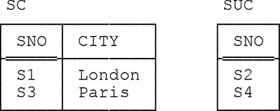
Fig. C.4: Horizontally decomposing table SC

As you can see, we now have two tables: (a) an abbreviated version of table SC (for which I’ve retained that same name SC, for convenience), containing just the original SC rows that had no shaded entries in column CITY; and (b) another table SUC (“suppliers with an unknown city”), containing just the original SC rows that did have shaded entries in column CITY— except that the CITY column in that table, if we kept it, would contain nothing but shaded entries, and so we can discard it without losing any information. The predicates for these two tables are as follows:

• SC:     Supplier SNO is located in city CITY.

• SUC: We don’t know where supplier SNO is located.

Observe in particular that the predicate for this new version of table SC has two parameters, SNO and CITY, and that table has two columns accordingly; by contrast, the predicate for table SUC has just one parameter, SNO, and that table has just one column accordingly.

Of course, we can and should perform an analogous horizontal decomposition on table ST from Fig. C.2. The result is shown in Fig. C.5.

C.5: Horizontally decomposing table ST

The predicates for the tables in Fig. C.5 are as follows:

• ST: Supplier SNO has status STATUS.

• SUT: We don’t know supplier SNO’s status.

Note: Each of tables SN (Fig. C.2), SC and SUC (in Fig. C.4), and ST and SUT (in Fig. C.5) is in fact “truly relational,” and so I could now switch to my preferred terminology of relations, tuples, and attributes. For simplicity, however, I’ll continue to use the terminology of tables, rows, and columns throughout the remainder of this appendix.

WHAT DO THE SHADED ENTRIES MEAN?

Let’s ignore status values for the moment and concentrate on cities. So far, then, I’ve said that shaded entries in the CITY column as shown in, e.g., Fig. C.2 mean we don’t know the applicable supplier city—i.e., the supplier does have a city, but we don’t know what it is. But our not knowing is only one of many possible reasons why we might not be able to use a genuine city name as some entry in that column. For example, it might be that the notion of having a city simply doesn’t apply to some suppliers (perhaps they conduct their business entirely online). If so, we might say, very loosely, that table SC, with those shaded entries in the CITY column (i.e., table SC as shown in Fig. C.2), has a predicate looking something like this:

Note, therefore, that those shaded entries now potentially have two distinct interpretations: Some of them mean we don’t know the applicable city, others mean the property of having a city doesn’t apply. So, again, we apply horizontal decomposition, this time to obtain three tables: SC (suppliers with a known city), SUC (suppliers with an unknown city), and SNC (suppliers with no city). If we assume for the sake of the example that supplier S2 has an unknown city and supplier S4 doesn’t have a city at all, the result of this decomposition is as shown in Fig. C.6.

Fig. C.6: Horizontally decomposing table SC, allowing for suppliers with no city

The predicates are:

• SC:     Supplier SNO is located in city CITY.

• SUC: We don’t know where supplier SNO is located.

• SNC: Supplier SNO doesn’t have a location.

In other words, the decomposition approach allows us to represent as many different kinds of missing information as we like. To be specific, if there are n distinct reasons for supplier cities to be missing, there’ll be n + 1 tables having to do with suppliers and cities. Two possible objections to the approach thus immediately spring to mind:

1. Aren’t some queries going to get awfully complex? For example, suppose we just want to retrieve everything in the database having to do with suppliers (the analog of “SELECT * FROM S” in SQL); aren’t we going to have to do a lot of joins, or (worse) outer joins?

2. Aren’t we going to wind up with an awful lot of tables?

I’ll come back to the first of these issues in the section “Queries,” later. As for the second, well, there are several points I want to make. Let C be an SQL column for which nulls are allowed. Then:

• If the nulls in column C all represent the same kind of missing information, and if the same is true for all such columns C, then the number of tables resulting from the decomposition approach is exactly the same as the number resulting from a good relational design. (To paraphrase something I said earlier, the presence of such a column C in a table T means table T is certainly not a relational table. Proper relational design requires elimination of such columns.)

• The situation is worse if the nulls in some such column C represent two or more distinct kinds of missing information but proper decomposition isn’t done. If it isn’t, there’ll certainly be fewer tables—but the apparent simplicity of such a design is spurious: Those tables aren’t relational, they don’t faithfully reflect the real world, they no longer have a clear predicate, and queries are more susceptible to errors of formulation or errors of interpretation or both.

• There’s a tactic we might consider, if we want to reduce the number of tables, which I’ll illustrate with reference to Fig. C.6. In terms of that example, the tactic would involve combining tables SUC and SNC into a single table with two columns, SNO and REASON, where REASON indicates the reason why the applicable supplier has no recorded city:

  ┌─────┬────────┐
  │ SNO │ REASON │
  ├═════┼────────┤
  │ S2  │ d/k    │
  │ S4  │ n/a    │
  └─────┴────────┘

  But now we have to define appropriate values, and spell out their interpretations, for column REASON (in the example, I’ve used d/k for “don’t know” and n/a for “not applicable”). In fact, if the decomposition approach requires n missing information tables, the combination approach requires n missing information reasons. So the combination approach is in some respects no less complex than the decomposition approach. (In this connection, see Exercise C.1 at the end of this appendix.)

CONSTRAINTS

So far, then, our suggested overall design for the running example looks like Fig. C.7 below.

Fig. C.7: Fully decomposing table S

I’m assuming here, and will continue to assume throughout the rest of this appendix, that there’s just one reason why STATUS values might be missing (viz., we don’t know the value) and just two reasons why CITY values might be missing (viz., either we don’t know the value or no such value exists). Note, however, that the design of Fig. C.7 requires certain constraints to be satisfied in order to hold it together, so to speak. To be specific, the following constraints need to be stated and enforced:

1. Each table has {SNO} as a key.

2. Each row in SN has a matching row in exactly one of ST and SUT, and conversely.

3. Each row in SN has a matching row in exactly one of SC, SUC, and SNC, and conversely.

Of course, the first of these is just a conventional key constraint on each of the six tables; it can thus be expressed by means of conventional KEY specifications. As for the other two, they can easily be expressed in Tutorial D using D_UNION, as follows:²

QUERIES

Now I return to the question I raised earlier: Given a design like that of Fig. C.7, aren’t some queries going to get awfully complex? In particular, what’s involved with that design in doing a query analogous to the “simple” SQL query SELECT * FROM S?

Before I address that issue, let me first point out that some queries—queries, I venture to suggest, that are more likely to be needed in practice than ones like SELECT * FROM S—are actually easier to formulate with the design of Fig. C.7. As a trivial example, the query “For suppliers for whom CITY is both applicable and known, get supplier numbers and cities” becomes just

SELECT SNO , CITY
FROM   SC

instead of:

SELECT SNO , CITY
FROM   S
WHERE  CITY IS NOT NULL

What’s more, the query “Get suppliers for whom CITY is applicable but unknown” is not only simpler with the design of Fig. C.7, it can’t be done at all with the original design of Fig. C.1. (In other words, not only does the design of Fig. C.1 not deal very well with the missing information problem in general, it actually manages to lose information!)

Be that as it may, let’s now consider the “SELECT * FROM S” question. More precisely, let’s see how a respectable version of the table in Fig. C.1 can be obtained from those in Fig. C.7—where by respectable, I mean the table will contain proper and informative data values everywhere (no shaded entries! no nulls!), as indicated in Fig. C.8 below.

Fig. C.8: Revised (respectable) version of table S

Now, however, I’ll switch to Tutorial D (doing the example in SQL would make it too hard to see the forest for the trees). I’ll show the solution a step at a time, using the values from Fig. C.7 as a basis for illustrating the result of each step in turn; then I’ll bring all the steps together at the end.

1. WITH ( t1 := EXTEND ST : { XSTATUS := CAST_AS_CHAR ( STATUS ) } ) :

   t1
   ┌─────┬────────┬─────────┐
   │ SNO │ STATUS │ XSTATUS │      /* STATUS values are integers,          */
   ├═════┼────────┼─────────┤      /* XSTATUS values are character strings */
   │ S1  │     20 │ 20      │
   │ S2  │     10 │ 10      │
   └─────┴────────┴─────────┘

2. WITH ( t2 := t1 { ALL BUT STATUS } ) :

   t2
   ┌─────┬─────────┐
   │ SNO │ XSTATUS │
   ├═════┼─────────┤
   │ S1  │ 20      │
   │ S2  │ 10      │
   └─────┴─────────┘

3. WITH ( t3 := EXTEND SUT : { XSTATUS := 'd/k' } ) :

   t3
   ┌─────┬─────────┐
   │ SNO │ XSTATUS │
   ├═════┼─────────┤
   │ S3  │ d/k     │
   │ S4  │ d/k     │
   └─────┴─────────┘

4. WITH ( t4 := UNION { t2 , t3 } ) :

   t4
   ┌─────┬─────────┐
   │ SNO │ XSTATUS │
   ├═════┼─────────┤
   │ S1  │ 20      │
   │ S2  │ 10      │
   │ S3  │ d/k     │
   │ S4  │ d/k     │
   └─────┴─────────┘

5. WITH ( t5 := SC RENAME { CITY AS XCITY } ) :

   t5
   ┌─────┬────────┐
   │ SNO │ XCITY  │
   ├═════┼────────┤
   │ S1  │ London │
   │ S3  │ Paris  │
   └─────┴────────┘

6. WITH ( t6 := EXTEND SUC : { XCITY := 'd/k' } ) :

   t6
   ┌─────┬────────┐
   │ SNO │ XCITY  │
   ├═════┼────────┤
   │ S2  │ d/k    │
   └─────┴────────┘

7. WITH ( t7 := EXTEND SNC : { XCITY := 'n/a' } ) :

   t7
   ┌─────┬────────┐
   │ SNO │ XCITY  │
   ├═════┼────────┤
   │ S4  │ n/a    │
   └─────┴────────┘

8. WITH ( t8 := UNION { t5 , t6 , t7 } ) :

   t8
   ┌─────┬────────┐
   │ SNO │ XCITY  │
   ├═════┼────────┤
   │ S1  │ London │
   │ S2  │ d/k    │
   │ S3  │ Paris  │
   │ S4  │ n/a    │
   └─────┴────────┘

9. WITH ( S := JOIN { SN , t4 , t8 } ) : S

   S
   ┌─────┬───────┬─────────┬────────┐
   │ SNO │ SNAME │ XSTATUS │ XCITY  │
   ├═════┼───────┼─────────┼────────┤
   │ S1  │ Smith │ 20      │ London │
   │ S2  │ Jones │ 10      │ d/k    │
   │ S3  │ Blake │ d/k     │ Paris  │
   │ S4  │ Clark │ d/k     │ n/a    │
   └─────┴───────┴─────────┴────────┘

   Putting all of these steps together and simplifying slightly, we have:

   WITH ( t1 := EXTEND ST : { XSTATUS := CAST_AS_CHAR ( STATUS ) } ,
          t2 := t1 { ALL BUT STATUS } ,
          t3 := EXTEND SUT : { XSTATUS := 'd/k' } ,
          t4 := UNION { t2 , t3 } ,
          t5 := SC RENAME { CITY AS XCITY } ,
          t6 := EXTEND SUC : { XCITY := 'd/k' } ,
          t7 := EXTEND SNC : { XCITY := 'n/a' } ,
          t8 := UNION { t5 , t6 , t7 } ,
          S  := JOIN { SN , t4 , t8 } ) :
   S

Now, it’s certainly true that this expression looks a little complicated (or tedious, at any rate), and it might look even more so if I hadn’t formulated it a step at a time, using WITH. However:

• Various shorthands could be defined, if desired, that could be used to simplify it.

• I frankly doubt whether tables such as that in Fig. C.8 would ever be wanted much in practice anyway, except perhaps as the basis for some kind of periodic report.

• In any case, the complexity, such as it is, can always be concealed by making the table a view.

MORE ON PREDICATES

Note: This section is based on material from Chapter 4 (“The Closed World Assumption”) of my book Logic and Databases: The Roots of Relational Theory (see Appendix G).

In this section, I show how it’s possible to get “don’t know” answers out of a database without nulls, even if there aren’t any tables like table SUC (suppliers with an unknown city) that explicitly represent the fact that something is unknown. For simplicity, suppose our database consists in its entirety of just table SC (suppliers with a known city), as shown in Fig. C.9 below.

Fig. C.9: Table SC (suppliers with a known city)

Now consider the following query on table SC:

Is supplier S1 in London?

In Tutorial D:³

( SC WHERE SNO = 'S1' AND CITY = 'London' ) { }

Clearly, this expression evaluates to either TABLE_DEE or TABLE_DUM (TABLE_DEE if supplier S1 is in London, TABLE_DUM otherwise). Note, therefore, that—as I mentioned briefly in Chapter 3—TABLE_DEE and TABLE_DUM can be interpreted as yes and no, respectively. Note too the implicit appeal to The Closed World Assumption!—in effect, we’re saying that if the row (S1,London) fails to appear in table SC, we’re allowed to conclude that it’s not the case that supplier S1 is in London.

Now, I said previously that the predicate for table SC was Supplier SNO is located in city CITY. But it isn’t—not really. To see why not, consider what happens if some user tries to introduce a new row into the table, perhaps as follows:

INSERT SC RELATION { TUPLE { SNO 'S6' , CITY 'Madrid' } } ;

In effect, the user here is telling the system there’s a new supplier, S6, with city Madrid. Now, the system obviously has no way of knowing whether the user’s assertion is true; as I explained in Chapter 8, all it can do (and does do) is check that the requested insertion, if performed, doesn’t cause any integrity constraints to be violated. If it doesn’t, then the system accepts the row, and interprets it as representing a true fact from this point forward.

We see, therefore, that rows in table SC don’t necessarily represent actual states of affairs in the real world; rather, they represent what the user tells the system about the real world, or in other words the user’s knowledge of the real world. Thus, the predicate for relvar SC isn’t really just Supplier SNO is located in city CITY; rather, it’s We know that supplier SNO is located in city CITY. And the effect of a successful INSERT is to make the system aware of something the user already knows. Thus, the database doesn’t contain the real world (of course not); what it contains is, rather, the system’s knowledge of the real world. And the system’s knowledge is derived in turn from the user’s knowledge (of course!—there’s no magic here).⁴

So when we pose a query to the system, by definition that query can’t be a query about the real world; instead, it is—it has to be—a query about the system’s knowledge of the real world. For example, consider again the query discussed above: Is supplier S1 in London? This rather imprecise natural language formulation has to be understood as shorthand for the following more accurate one:

Do we know that supplier S1 is in London?

In practice, of course, we almost never talk in such precise terms; we usually elide qualifiers like “Do we know that” (or “According to the system’s knowledge, is it true that,” or “Does the database say that,” and so on). But even if we do elide them, we certainly need to understand that, conceptually, they’re there—for otherwise we’ll be really confused. (Though perhaps I should add that such confusions aren’t exactly unknown in practice.)

It follows from the foregoing discussion that the Tutorial D expression I showed earlier—

( SC WHERE SNO = 'S1' AND CITY = 'London' ) { }

—doesn’t really represent the query Is supplier S1 in London? after all. Rather, it represents the query Do we know that supplier S1 is in London? And, appealing again to The Closed World Assumption, it follows further that:

• If the result is TABLE_DEE (yes), it means we do know supplier S1 is in London.

• If the result is TABLE_DUM (no), it means we don’t know whether supplier S1 is in London. And that’s a “don’t know” answer if ever you saw one.

Of course, if a row for supplier S1 does appear in the table but the CITY value in that row isn’t London, we know that supplier S1 isn’t in London (I’m appealing here to the fact that {SNO} is a key for table SC). Putting it all together, then, we have the following:

• If a row for supplier S1 appears in table SC and the CITY value in that row is London, it means yes, we know supplier S1 is in London.

• If a row for supplier S1 appears in table SC but the CITY value in that row is something other than London, it means no, we know supplier S1 isn’t in London.

• And if no row for supplier S1 appears in table SC at all, it means we don’t know whether supplier S1 is in London.

Given The Closed World Assumption, then, we can formulate queries that return a true / false / unknown answer, and we don’t need nulls or 3VL to do so. Here’s a Tutorial D formulation for the example under discussion:

( EXTEND ( SC WHERE SNO = 'S1' AND CITY = 'London' ) { } :
                             { RESULT := 'true ' } ) { RESULT }
  UNION
( EXTEND ( SC WHERE SNO = 'S1' AND CITY ≠ 'London' ) { } :
                             { RESULT := 'false ' } ) { RESULT }
  UNION
( EXTEND ( RELATION { TUPLE { SNO 'S1' } } MINUS SC { SNO } ) { } :
                             { RESULT := 'unknown' } ) { RESULT }

As you can see, this expression takes the form a UNION b UNION c, where each of a, b, and c is a table of just one column, called RESULT. Moreover, it should be clear that exactly one of a, b, and c contains just one row and the other two contain no rows at all. The overall result is thus a one-column, one-row table; the single column, RESULT, is of type character string, and the single row contains the appropriate RESULT value. And the trick—though it isn’t really a trick at all—is that the RESULT value is a character string, not a truth value. As a consequence, there’s no need to get into the 3VL quagmire in order to formulate queries that can yield “true,” “false,” or “unknown” answers, if that’s what we really want.

For completeness, here’s an SQL analog of the foregoing Tutorial D expression:

SELECT 'true    ' AS RESULT
FROM ( SELECT *
       FROM   SC
       WHERE  SNO = 'S1'
       AND    CITY = 'London' ) AS POINTLESS1
UNION  CORRESPONDING
SELECT 'false ' AS RESULT
FROM ( SELECT *
       FROM   SC
       WHERE  SNO = 'S1'
       AND    CITY <> 'London' ) AS POINTLESS2
UNION  CORRESPONDING
SELECT 'unknown' AS RESULT
FROM ( VALUES ('S1' )
       EXCEPT
       SELECT SNO
       FROM   SC ) AS POINTLESS3

Incidentally, if you’re wondering about those AS POINTLESS specifications in this SQL expression, I remind you from Chapter 7 (or Chapter 12) that SQL has a syntax rule to the effect that a table subquery in the FROM clause must be accompanied by an explicit AS clause that defines an associated range variable, even if that range variable is never explicitly referenced anywhere in the overall expression. Note also that specifying CORRESPONDING on the EXCEPT in the final portion of this expression would actually be incorrect! It could be made correct by replacing the specification VALUES ('S1') by an expression of the form SELECT DISTINCT 'S1' AS SNO FROM T where T is some arbitrary—but nonempty—named table.

EXERCISES

C.1 Give an appropriate predicate for the table shown near the top of page 500 (with columns SNO and REASON).

C.2 Give SQL versions of constraints EQD2 and EQD3 from the section “Constraints” in the body of the appendix.

C.3 Give an SQL version of the Tutorial D expression near the end of the section “Queries” in the body of the appendix.

C.4 Why would it be incorrect to specify CORRESPONDING on the EXCEPT in the final portion of the SQL expression at the end of the section immediately preceding these exercises?

ANSWERS

C.1 REASON is either 'd/k' or 'n/a', and if REASON is 'd/k' then we don’t know where supplier SNO is located, and if REASON is 'n/a' then supplier SNO doesn’t have a location.

C.2 Here’s an SQL version of constraint EQD2 (only; constraint EQD3 is essentially similar, of course).

CREATE ASSERTION EQD2 CHECK
     ( NOT EXISTS ( SELECT SNO
                    FROM   ST
                    WHERE  SNO IN ( SELECT SNO
                                    FROM   SUT ) )
       AND
       NOT EXISTS ( SELECT SNO
                    FROM   SUT
                    WHERE  SNO IN ( SELECT SNO
                                    FROM   ST ) )
       AND
       NOT EXISTS ( SELECT SNO
                    FROM   SN
                    WHERE  SNO NOT IN ( SELECT SNO
                                        FROM   ST
                                        UNION  CORRESPONDING
                                        SELECT SNO
                                        FROM   SUT ) )
       AND
       NOT EXISTS ( SELECT SNO
                    FROM ( SELECT SNO
                           FROM   ST
                           UNION  CORRESPONDING
                           SELECT SNO
                           FROM   SUT ) AS POINTLESS
                    WHERE  SNO NOT IN ( SELECT SNO
                                        FROM   SN ) ) ) ;

C.3

WITH t1 AS ( SELECT SNO , STATUS ,                     CAST ( STATUS AS CHAR ( 3 ) ) AS XSTATUS              FROM   ST ) ,      t2 AS ( SELECT SNO , XSTATUS              FROM   t1 ) ,      t3 AS ( SELECT SNO , 'd/k' AS XSTATUS              FROM   SUT ) ,      t4 AS ( SELECT SNO , XSTATUS              FROM   t1              UNION  CORRESPONDING              SELECT SNO , XSTATUS              FROM   t3 ) ,      t5 AS ( SELECT SNO , CITY AS XCITY              FROM   SC ) ,      t6 AS ( SELECT SNO , 'd/k' AS XCITY              FROM   SUC ) ,      t7 AS ( SELECT SNO , 'n/a' AS XCITY              FROM   SNC ) ,      t8 AS ( SELECT SNO , XCITY              FROM   t5              UNION  CORRESPONDING              SELECT SNO , XCITY              FROM   t6              UNION  CORRESPONDING              SELECT SNO , XCITY              FROM   t7 ) , S  AS ( SELECT SNO , SNAME , XSTATUS , XCITY         FROM   SN NATURAL JOIN t4 NATURAL JOIN t8 ) SELECT SNO , SNAME , XSTATUS , XCITY FROM   S

C.4 Because CORRESPONDING means “match on column names” and the single column in the table produced by the expression VALUES('S1') doesn’t have a name.