Chapter 2: Flash Distillation

2.1 Basic Method of Flash Distillation

One of the simplest separation processes commonly employed is flash distillation. In this process, part of a feed stream vaporizes in a flash chamber, and the vapor and liquid in equilibrium with each other are separated. The more volatile component will be more concentrated in the vapor. Usually a large degree of separation is not achieved; however, in some cases, such as the desalination of seawater, complete separation results.

The equipment needed for flash distillation is shown in Figure 2-1. The fluid is pressurized and heated and is then passed through a throttling valve or nozzle into the flash drum. Because of the large drop in pressure, part of the fluid vaporizes. The vapor is taken off overhead, while the liquid drains to the bottom of the drum, where it is withdrawn. A demister or entrainment eliminator is often employed to prevent liquid droplets from being entrained in the vapor. The system is called “flash” distillation because the vaporization is extremely rapid after the feed enters the drum. Because of the intimate contact between liquid and vapor, the system in the flash chamber is very close to an equilibrium stage. Figure 2-1 shows a vertical flash drum, but horizontal drums are also common.

Figure 2-1 Flash distillation system

The designer of a flash system needs to know the pressure and temperature of the flash drum, the size of the drum, and the liquid and vapor compositions and flow rates. He or she also wishes to know the pressure, temperature, and flow rate of the feed entering the drum. In addition, he or she will need to know how much the original feed has to be pressurized and heated. The pressures must be chosen so that at the feed pressure, p_F, the feed is below its boiling point and remains liquid, while at the pressure of the flash drum, p_drum, the feed is above its boiling point and some of it vaporizes. If the feed is already hot and/or the pressure of the flash drum is quite low, the pump and heater shown in Figure 2-1 may not be needed.

The designer has six degrees of freedom to work with for a binary separation. Usually, the original feed specifications take up four of these degrees of freedom:

Feed flow rate, F

Feed composition, z (mole fraction of the more volatile component)

Temperature, T₁

Pressure, p₁

Of the remaining, the designer will usually select first

Drum pressure, p_drum

A number of other variables are available to fulfill the last degree of freedom.

As is true in the design of many separation techniques, the choice of specified design variables controls the choice of the design method. For the flash chamber, we can use either a sequential solution method or a simultaneous solution method. In the sequential procedure, we solve the mass balances and equilibrium relationships first and then solve the energy balances and enthalpy equations. In the simultaneous solution method, all equations must be solved at the same time. In both cases we solve for flow rates, compositions, and temperatures before we size the flash drum.

We will assume that the flash drum shown in Figure 2-1 acts as an equilibrium stage. Then vapor and liquid are in equilibrium. For a binary system the mole fraction of the more volatile component in the vapor y and its mole fraction in the liquid x and T_drum can be determined from the equilibrium expressions:

(2-1)

(2-2)

To use Eqs. (2-1) and (2-2) in the design of binary flash distillation systems, we must take a short tangent and first discuss binary vapor-liquid equilibrium (VLE).

2.2 Form and Sources of Equilibrium Data

Equilibrium data is required to understand and design the separations in Chapters 1 to 15 and 17. In principle, we can always experimentally determine the VLE data we require. For a simple experiment we could take a chamber similar to Figure 1-2 and fill it with the chemicals of interest. Then, at different pressures and temperatures, allow the liquid and vapor sufficient time to come to equilibrium and then take samples of liquid and vapor and analyze them. If we are very careful we can obtain reliable equilibrium data. In practice, the measurement is fairly difficult and a variety of special equilibrium stills have been developed. Marsh (1978) and Van Ness and Abbott (1982, section 6-7) briefly review methods of determining equilibrium. With a static equilibrium cell, concentration measurements are not required for binary systems. Concentrations can be calculated from pressure and temperature data, but the calculation is complex.

If we obtained equilibrium measurements for a binary mixture of ethanol and water at 1 atm, we would generate data similar to those shown in Table 2-1. The mole fractions in each phase must sum to 1.0. Thus for this binary system,

(2.3)

where x is mole fraction in the liquid and y is mole fraction in the vapor. Very often only the composition of the most volatile component (ethanol in this case) will be given. The mole fraction of the less volatile component can be found from Eqs. (2-3). Equilibrium depends on pressure. (Data in Table 2-1 are specified for a pressure of 1 atm.) Table 2-1 is only one source of equilibrium data for the ethanol-water system, and over a dozen studies have explored this system (Wankat, 1988), and data are contained in the more general sources listed in Table 2-2. The data in different references do not agree perfectly, and care must be taken in choosing good data. We will refer back to this (and other) data quite often. If you have difficulty finding it, look in the index under ethanol–water VLE.

Table 2-1. Vapor-liquid equilibrium data for ethanol and water at 1 atm y and x in Mole Fractions

xEtoh	xw	yetoh	yw	T,° C
0	1.0	0	1.0	100
0.019	0.981	0.170	0.830	95.5
0.0721	0.9279	0.3891	0.6109	89.0
0.0966	0.9034	0.4375	0.5625	86.7
0.1238	0.8762	0.4704	0.5296	85.3
0.1661	0.8339	0.5089	0.4911	84.1
0.2337	0.7663	0.5445	0.4555	82.7
0.2608	0.7392	0.5580	0.4420	82.3
0.3273	0.6727	0.5826	0.4174	81.5
0.3965	0.6035	0.6122	0.3878	80.7
0.5198	0.4802	0.6599	0.3401	79.7
0.5732	0.4268	0.6841	0.3159	79.3
0.6763	0.3237	0.7385	0.2615	78.74
0.7472	0.2528	0.7815	0.2185	78.41
0.8943	0.1057	0.8943	0.1057	78.15
1.00	0	1.00	0	78.30

R.H. Perry, C.H. Chilton and S.O. Kirkpatrick (Eds.), Chemical Engineers Handbook, 4th ed., New York, McGraw-Hill, p. 13-5, 1963.

Table 2-2. Sources of vapor-liquid equilibrium data

Chu, J.C., R.J. Getty, L.F. Brennecke, and R. Paul, Distillation Equilibrium Data, Reinhold, New York, 1950.

Engineering Data Book, Natural Gasoline Supply Men’s Association, 421 Kennedy Bldg., Tulsa, Oklahoma, 1953.

Hala, E., I. Wichterle, J. Polak, and T. Boublik, Vapor-Liquid Equilibrium Data at Normal Pressures, Pergamon, New York, 1968.

Hala, E., J. Pick, V. Fried, and O. Vilim, Vapor-Liquid Equilibrium, 3rd ed., 2nd Engl. ed., Pergamon, New York, 1967.

Horsely, L.H., Azeotropic Data, ACS Advances in Chemistry, No. 6, American Chemical Society, Washington, DC, 1952.

Horsely, L.H. Azeotropic Data (II), ACS Advances in Chemistry, No. 35, American Chemical Society, Washington, DC, 1952.

Gess, M.A., R.P. Danner and M. Nagvekar, Thermodynamic Analysis of Vapor-Liquid Equilibria: Recommended Models and a Standard Data Base, DIPPR, AIChE, New York, 1991.

Gmehling, J., J. Menke, J. Krafczyk and K. Fischer, Azeotropic Data, VCH Weinheim, Germany, 1994.

Gmehling, J., U. Onken, W. Arlt, P. Grenzheuser, U. Weidlich, B. Kolbe, J.R. Rarey-Nies, DECHEMA Chemistry Data Series, Vol. I, Vapor-Liquid Equilibrium Data Collection, DECHEMA, Frankfurt (Main), Germany, 1977-1984.

Maxwell, J.B., Data Book on Hydrocarbons, Van Nostrand, Princeton, New Jersey, 1950.

Perry, R.H. and Green, D. (Eds.), Perry’s Chemical Engineer’s Handbook, 7^th ed., McGraw-Hill, New York, 1997.

Prausnitz, J.M., Anderson, T.F., Grens, E.A., Eckert, C.A., Hsieh, R., and O’Connell, J.P., Computer Calculations for Multicomponent Vapor-Liquid and Liquid-Liquid Equilibria, Prentice-Hall, Upper Saddle River, NJ, 1980.

Stephan, K. and H. Hildwein, DECHEMA Chemistry Data Series, Vol. IV, Recommended Data of Selected Compounds and Binary Mixtures, DECHEMA, Frankfurt (Main), Germany, 1987.

Timmermans, J., The Physico-Chemical Constants of Binary Systems in Concentrated Solutions, 5 vols., Interscience, New York, 1959-1960.

Van Winkle, M., Distillation, McGraw-Hill, New York, 1967.

Wichterle, I., J. Linek and E. Hala, Vapor-Liquid Equilibrium Data Bibliography, Elsevier, Amsterdam, 1973.

We see in Table 2-1 that if pressure and temperature are set, then there is only one possible vapor composition for ethanol, y_Etoh, and one possible liquid composition, x_Etoh. Thus we cannot arbitrarily set as many variables as we might wish. For example, at 1 atm we cannot arbitrarily decide that we want vapor and liquid to be in equilibrium at 95° C and x_Etoh = 0.1.

The number of variables that we can arbitrarily specify, known as the degrees of freedom, is determined by subtracting the number of thermodynamic equilibrium equations from the number of variables. For nonreacting systems the resulting Gibbs phase rule is

(2-4)

where F = degrees of freedom, C = number of components, and P = number of phases. For the binary system in Table 2-1, C = 2 (ethanol and water) and P = 2 (vapor and liquid). Thus,

F = 2 − 2 + 2 = 2

When pressure and temperature are set, all the degrees of freedom are used, and at equilibrium all compositions are determined from the experiment. Alternatively, we could set pressure and x_Etoh or x_W and determine temperature and the other mole fractions.

The amount of material and its flow rate are not controlled by the Gibbs phase rule. The phase rule refers to intensive variables such as pressure, temperature, or mole fraction, which do not depend on the total amount of material present. The extensive variables, such as number of moles, flow rate, and volume, do depend on the amount of material and are not included in the degrees of freedom. Thus a mixture in equilibrium must follow Table 2-1, whether there are 0.1, 1.0, 10, 100, or 1,000 moles present.

Binary systems with only two degrees of freedom can be conveniently represented in tabular or graphical form by setting one variable (usually pressure) constant. VLE data have been determined for many binary systems. Sources for these data are listed in Table 2-2; you should become familiar with several of these sources. Note that the data are not of equal quality. Methods for testing the thermodynamic consistency of equilibrium data are discussed in detail by Barnicki (2002), Walas (1985), and Van Ness and Abbott (1982, pp. 56-64, 301-348). Errors in the equilibrium data can have a profound effect on the design of the separation method (e.g., see Nelson et al., 1983 or Carlson, 1996).

2.3 Graphical Representation of Binary VLE

Binary VLE data can be represented graphically in several ways. The most convenient forms are temperature-composition, y-x, and enthalpy-composition diagrams. These figures all represent the same data and can be converted from one form to another.

Table 2-1 gives the equilibrium data for ethanol and water at 1 atmosphere. With pressure set, there is only one degree of freedom remaining. Thus we can select any of the intensive variables as the independent variable and plot any other intensive variable as the dependent variable. The simplest such graph is the y vs. x graph shown in Figure 2-2. Typically, we plot the mole fraction of the more volatile component (the component that has y > x; ethanol in this case). This diagram is also called a McCabe-Thiele diagram when it is used for calculations. Pressure is constant, but the temperature is different at each point on the equilibrium curve. Points on the equilibrium curve represent two phases in equilibrium. Any point not on the equilibrium curve represents a system that may have both liquid and vapor, but they are not in equilibrium. As we will discover later, y-x diagrams are extremely convenient for calculation.

Figure 2-2 y vs. x diagram for ethanol-water

The data in Table 2-1 can also be plotted on a temperature-composition diagram as shown in Figure 2-3. The result is actually two graphs: One is liquid temperature vs. x_Etoh, and the other is vapor temperature vs. y_Etoh. These curves are called saturated liquid and saturated vapor lines, because they represent all possible liquid and vapor systems that can be in equilibrium at a pressure of 1 atm. Any point below the saturated liquid curve represents a subcooled liquid (liquid below its boiling point) whereas any point above the saturated vapor curve would be a superheated vapor. Points between the two saturation curves represent streams consisting of both liquid and vapor. If allowed to separate, these streams will give a liquid and vapor in equilibrium. Liquid and vapor in equilibrium must be at the same temperature; therefore, these streams will be connected by a horizontal isotherm as shown in Figure 2-3 for x_Etoh = 0.2.

Figure 2-3 Temperature-composition diagram for ethanol-water

Even more information can be shown on an enthalpy-composition or Ponchon-Savarit diagram, as illustrated for ethanol and water in Figure 2-4. Note that the units in Figure 2-4 differ from those in Figure 2-3. Again, there are really two plots: one for liquid and one for vapor. The isotherms shown in Figure 2-4 show the change in enthalpy at constant temperature as weight fraction varies. Because liquid and vapor in equilibrium must be at the same temperature, these points are connected by an isotherm. Points between the saturated vapor and liquid curves represent two-phase systems. An isotherm through any point can be generated using the auxiliary line with the construction shown in Figure 2-5. To find an isotherm, go vertically from the saturated liquid curve to the auxiliary line. Then go horizontally to the saturated vapor line. The line connecting the points on the saturated vapor and saturated liquid curves is the isotherm. If an isotherm is desired through a point in the two-phase region, a simple trial-and-error procedure is required.

Figure 2-4 Enthalpy-composition diagram for ethanol-water at a pressure of 1 kg/cm² (Bosnjakovic, Technische Thermodynamik, T. Steinkopff, Leipzig, 1935)

Figure 2-4 Use of auxiliary line

Isotherms on the enthalpy-composition diagram can also be generated from the y-x and temperature-composition diagrams. Since these diagrams represent the same data, the vapor composition in equilibrium with a given liquid composition can be found from either the y-x or temperature-composition graph, and the value transferred to the enthalpy-composition diagram. This procedure can also be done graphically as shown in Figure 2-6 if the units are the same in all figures. In Figure 2-6a we can start at point A and draw a vertical line to point A′ (constant x value). At constant temperature, we can find the equilibrium vapor composition (point B′). Following the vertical line (constant y), we proceed to point B. The isotherm connects points A and B. A similar procedure is used in Figure 2-6b, except now the y-x line must be used on the McCabe-Thiele graph. This is necessary because points A and B in equilibrium appear as a single point, A′/B′, on the y-x graph. The y = x line allows us to convert the ordinate value (y) on the y-x diagram to an abscissa value (also y) on the enthalpy-composition diagram. Thus the procedure is to start at point A and go up to point A′/B′ on the y-x graph. Then go horizontally on the y = x line and finally drop vertically to point B on the vapor curve. The isotherm now connects points A and B.

Figure 2-6 Drawing isotherms on the enthalpy-composition diagram A) from the temperature-composition diagram; B) from the y-x diagram

The data presented in Table 2-1 and illustrated in Figures 2-2, 2-3, and 2-4 show a minimum-boiling azeotrope, i.e., the liquid and vapor are of exactly the same composition at a mole fraction ethanol of 0.8943. This can be found from Figure 2-2 by drawing the y = x line and finding the intersection with the equilibrium curve. In Figure 2-3 the saturated liquid and vapor curves touch, while in Figure 2-4 the isotherm is vertical at the azeotrope. Note that the azeotrope composition is numerically different in Figure 2-4, but actually it is essentially the same, since Figure 2-4 is in wt frac, whereas the other figures are in mole fractions. Below the azeotrope composition, ethanol is the more volatile component; above it, ethanol is the less volatile component. The system is called a minimum-boiling azeotrope because the azeotrope boils at 78.15° C, which is less than that of either pure ethanol or pure water. The azeotrope location is a function of pressure. Below 70 mmHg no azeotrope exists for ethanol-water. Maximum-boiling azeotropes also occur (see Figure 2-7). Only the temperature-composition diagram will look significantly different. Another type of azeotrope occurs when there are two partially miscible liquid phases. Equilibrium for partially miscible systems is considered in Chapter 8.

Figure 2-7 Maximum boiling azeotrope system

2.4 Binary Flash Distillation

We will now use the binary equilibrium data to develop graphical and analytical procedures to solve the combined equilibrium, mass balance and energy balance equations. Mass and energy balances are written for the balance envelope shown as a dashed line in Figure 2-1. For a binary system there are two independent mass balances. The standard procedure is to use the overall mass balance,

(2-5)

and the component balance for the more volatile component,

(2-6)

The energy balance is

(2-7)

where h_F, H_v and h_L are the enthalpies of the feed, vapor, and liquid streams. Usually Q_flash = 0, since the flash drum is insulated and the flash is considered to be adiabatic.

To use the energy balance equations, we need to know the enthalpies. Their general form is

(2-8)

For binary systems it is often convenient to represent the enthalpy functions graphically on an enthalpy-composition diagram such as Figure 2-4. For ideal mixtures the enthalpies can be calculated from heat capacities and latent heats. Then,

(2-9a)

(2-9b)

(2-10)

where x_A and y_A are mole fractions of component A in liquid and vapor, respectively. C_P is the molar heat capacity, T_ref is the chosen reference temperature, and λ is the latent heat of vaporization at T_ref. For binary systems, x_B = 1 − x_A, and y_B = 1 − y_A.

2.4.1 Sequential Solution Procedure

In the sequential solution procedure, we first solve the mass balance and equilibrium relationships, and then we solve the energy balance and enthalpy equations. In other words, the two sets of equations are uncoupled. The sequential solution procedure is applicable when the last degree of freedom is used to specify a variable that relates to the conditions in the flash drum. Possible choices are:

Vapor mole fraction, y

Liquid mole fraction, x

Fraction feed vaporized, f = V/F

Fraction feed remaining liquid, q = L/F

Temperature of flash drum, T_drum

If one of the equilibrium conditions, y, x, or T_drum, is specified, then the other two can be found from Eqs. (2-3) and (2-4) or the graphical representation of equilibrium data. For example, if y is specified, x is obtained from Eq. (2-3) and T_drum from Eq. (2-4). In the mass balances, Eqs. (2-5) and (2-6), the only unknowns are L and V, and the two equations can be solved simultaneously.

If either the fraction vaporized or fraction remaining liquid is specified, Eqs. (2-3), (2-4), and (2-6) must be solved simultaneously. The most convenient way to do this is to combine the mass balances. Solving Eq. (2-6) for y, we obtain

(2-11)

Equation (2-11) is the operating equation, which for a single-stage system relates the compositions of the two streams leaving the stage. Equation (2-11) can be rewritten in terms of either the fraction vaporized, f = V/F, or the fraction remaining liquid, q = L/F.

From the overall mass balance, Eq. (2-5),

(2-12)

Then the operating equation becomes

(2-13)

The alternative in terms of L/F is

(2-14)

and the operating equation becomes

(2-15)

Although they have different forms Eqs. (2-11), (2-13), and (2-15) are equivalent means of obtaining y, x, or z. We will use whichever operating equation is most convenient.

Now the equilibrium Eq. (2-3) and the operating equation (Eq. 2-11, 2-13, or 2-15) must be solved simultaneously. The exact way to do this depends on the form of the equilibrium data. For binary systems a graphical solution is very convenient. Equations (2-11), (2-13), and (2-15) represent a single straight line, called the operating line, on a graph of y vs. x. This straight line will have

(2-16)

and

(2-17)

The equilibrium data at pressure p_drum can also be plotted on the y-x diagram. The intersection of the equilibrium curve and the operating line is the simultaneous solution of the mass balances and equilibrium. This plot of y vs. x showing both equilibrium and operating lines is called a McCabe-Thiele diagram and is shown in Figure 2-8 for an ethanol-water separation. The equilibrium data are from Table 2-1 and the equilibrium curve is identical to Figure 2-2. The solution point gives the vapor and liquid compositions leaving the flash drum. Figure 2-8 shows three different operating lines as V/F varies from 0 to to 1.0 (see Example 2-1). T_drum can be found from Eq. (2-4) or from a temperature-composition diagram.

Figure 2-8. McCabe-Thiele diagram for binary flash distillation; illustrated for Example 2-1

Two other points shown on the McCabe-Thiele diagram are the x intercept (y = 0) of the operating line and its intersection with the y = x line. Either of these points can also be located algebraically and then used to plot the operating line.

The intersection of the operating line and the y = x line is often used because it is simple to plot. This point can be determined by simultaneously solving Eq. (2-11) and the equation y = x. Substituting y = x into Eq. (2-11), we have

or

or

since V + L = F, the result is y = z and therefore

x = y = z

The intersection is at the feed composition.

It is important to realize that the y = x line has no fundamental significance. It is often used in graphical solution methods because it simplifies the calculation. However, do not use it blindly.

Obviously, the graphical technique can be used if y, x, or T_drum is specified. The order in which you find points on the diagram will depend on what information you have to begin with.

Example 2-1. Flash separator for ethanol and water

A flash distillation chamber operating at 101.3 kPa is separating an ethanol-water mixture. The feed mixture is 40 mole % ethanol. (a) What is the maximum vapor composition and (b) what is the minimum liquid composition that can be obtained if V/F is allowed to vary? (c) If V/F = 2/3, what are the liquid and vapor compositions? (d) Repeat step c, given that F is specified as 1,000 kg moles/hr.

Solution

A. Define. We wish to analyze the performance of a flash separator at 1 atm.

a. Find y_max.

b. Find x_min.

c. and d. Find y and x for V/F = 2/3.

B. Explore. Note that p_drum = 101.3 kPa = 1 atm. Thus we must use data at this pressure. These data are conveniently available in Table 2-1 and Figure 2-2. Since p_drum and V/F for part c are given, a sequential solution procedure will be used. For parts a and b we will look at limiting values of V/F.

C. Plan. We will use the y-x diagram as illustrated in Figure 2-2. For all cases we will do a mass balance to derive an operating line [we could use Eqs. (2-11), (2-13), or (2-15), but I wish to illustrate deriving an operating line]. Note that 0 ≤ V/F ≤ 1.0. Thus our maximum and minimum values for V/F must lie within this range.

D. Do It. Sketch is shown.

Mass Balances:	F = V + L
	Fz = Vy + Lx

Solve for y:

From the overall balance, L = F − V. Thus

when V/F = 0.0, V = 0, L = F, and L/V = F/0 = ∞

when V/F = 2/3, V = (2/3)F, L = (1/3)F, and L/V = (1/3)F/[(2/3)F] = 1/2

when V/F = 1.0, V = F, L = 0, and L/V = 0/F = 0

Thus the slopes (−L/V) are −∞, −1/2, and −0.

If we solve for the y = x interception, we find it at y = x = z = 0.4 for all cases. Thus we can plot three operating lines through y = x = z = 0.4, with slopes of −∞, −1/2 and −0. These operating lines were shown in Figure 2-8.

a. Highest y is for V/F = 0: y = 0.61 [x = 0.4]

b. Lowest x is for V/F = 1.0: x = 0.075 [y = 0.4]

c. When V/F is 2/3, y = 0.52 and x = 0.17

d. When F = 1,000 with V/F = 2/3, the answer is exactly the same as in part c. The feed rate will affect the drum diameter and the energy needed in the preheater.

E. Check. We can check the solutions with the mass balance, Fz = Vy + Lx.

a. (100)(0.4) = 0(0.61) + (100)(0.4) checks

b. (100)(0.4) = 100(0.4) + (0)(0.075) checks

c. 100(0.4) = (66.6)(0.52) + (33.3)(0.17)

Note V = (2/3)F and L = (1/3)F

This is 40 = 39.9, which checks within the accuracy of the graph

d. Check is similar to c: 400 = 399

We can also check by fitting the equilibrium data to a cubic equation and then simultaneously solve equilibrium and operating equations by minimizing the residual. These spread sheet calculations agree with the graphical solution.

F. Generalization. The method for obtaining bounds for the answer (setting the V/F equation to its extreme values of 0.0 and 1.0) can be used in a variety of other situations. In general, the feed rate will not affect the compositions obtained in the design of stage separators. Feed rate does not affect heat requirement and equipment diameters.

Once the conditions within the flash drum have been calculated, we proceed to the energy balance. With y, x, and T_drum known, the enthalpies H_v and h_L are easily calculated from Eqs. (2-8) or (2-9) and (2-10). Then the only unknown in Eq. (2-7) is the feed enthalpy h_F. Once h_F is known, the inlet feed temperature T_F can be obtained from Eq. (2-8) or (2-9b).

The amount of heat required in the heater, Q_h, can be determined from an energy balance around the heater.

(2-19)

Since enthalpy h₁ can be calculated from T₁ and z, the only unknown is Q_h, which controls the size of the heater.

The feed pressure, p_F, required is semi-arbitrary. Any pressure high enough to prevent boiling at temperature T_F can be used.

One additional useful result is the calculation of V/F when all mole fractions (z, y, x) are known. Solving Eqs. (2-5) and (2-6), we obtain

(2-20)

Except for sizing the flash drum, which is covered later, this completes the sequential procedure. Note that the advantages of this procedure are that mass and energy balances are uncoupled and can be solved independently. Thus trial-and-error is not required.

If we have a convenient equation for the equilibrium data, then we can obtain the simultaneous solution of the operating equation (2-9, 2-11, or 2-13) and the equilibrium equation analytically. For example, ideal systems often have a constant relative volatility α_AB where α_AB is defined as,

(2-21)

For binary systems,

y_B = 1 − y_A, x_B = 1 − x_A

and the relative volatility is

(2-22a)

Solving Eq. (2-22) for y_A, we obtain

(2-22b)

If Raoult’s law is valid, then we can determine relative volatility as

(2-23)

The relative volatility α may also be fit to experimental data.

If we solve Eqs. (2-21) and (2-11) simultaneously, we obtain

(2-24)

which is easily solved with the quadratic equation. This can be done conveniently with a spread sheet.

2.4.2 Simultaneous Solution Procedure

If the temperature of the feed to the drum, T_F, is the specified variable, the mass and energy balances and the equilibrium equations must be solved simultaneously. You can see from the energy balance, Eq. (2-7) why this is true. The feed enthalpy, h_F, can be calculated, but the vapor and liquid enthalpies, H_v and h_L, depend upon T_drum, y, and x, which are unknown. Thus a sequential solution is not possible.

We could write Eqs. (2-3) to (2-8) and solve seven equations simultaneously for the seven unknowns y, x, L, V, H_v, h_L, and T_drum. This is feasible but rather difficult, particularly since Eqs. (2-3) and (2-4) and often Eqs. (2-8) are nonlinear, so we resort to a trial-and-error procedure. This method is: Guess the value of one of the variables, calculate the other variables, and then check the guessed value of the trial variable. For a binary system, we can select any one of several trial variables, such as y, x, T_drum, V/F, or L/F. For example, if we select the temperature of the drum, T_drum, as the trial variable, the calculation procedure is:

1. Calculate h_F(T_F, z) [e.g., use Eq. (2-9b)].

2. Guess the value of T_drum.

3. Calculate x and y from the equilibrium equations (2-3) and (2-4) or graphically (use temperature-composition diagram).

4. Find L and V by solving the mass balance equations (2-5) and (2-6), or find L/V from Figure 2-8 and use the overall mass balance, Eq. (2-5).

5. Calculate h_L(T_drum, x) and H_v(T_drum, y) from Eqs. (2-8) or (2-9a) and (2-10) or from the enthalpy-composition diagram.

6. Check: Is the energy balance equation (2-7) satisfied? If it is satisfied we are finished. Otherwise, return to step 2.

The procedures are similar for other trial variables.

For binary flash distillation, the simultaneous procedure can be conveniently carried out on an enthalpy-composition diagram. First calculate the feed enthalpy, h_F, from Eq. (2-8) or Eq. (2-9b); then plot the feed point as shown on Figure 2-9 (see Problem 2-A1). In the flash drum the feed separates into liquid and vapor in equilibrium. Thus the isotherm through the feed point, which must be the T_drum isotherm, gives the correct values for x and y. The flow rates, L and V, can be determined from the mass balances, Eqs. (2-5) and (2-6), or from a graphical mass balance.

Figure 2-9 Binary flash calculation in enthalpy-composition diagram

Determining the isotherm through the feed point requires a minor trial-and-error procedure. Pick a y (or x), draw the isotherm, and check whether it goes through the feed point. If not, repeat with a new y (or x).

A graphical solution to the mass balances and equilibrium can be developed for Figure 2-9. Substitute the overall balance Eq. (2-5) into the more volatile component mass balance Eq. (2-6),

Lz + Vz = Lx + Vy

Rearranging and solving for L/V

(2-25)

Using basic geometry (y − z) is proportional to the distance and (z − x) is proportional to the distance . Then,

(2-26)

Equation (2-26) is called the lever-arm rule because the same result is obtained when a moment-arm balance is done on a seesaw. Thus if we set moment arms of the seesaw in Figure 2-10 equal, we obtain

or

which gives the same result as Eq. (2-26). The seesaw is a convenient way to remember the form of the lever-arm rule.

Figure 2.10. Illustration of lever-arm rule

The lever-arm rule can also be applied on enthalpy-composition diagrams and on ternary diagrams for extraction, where it has several other uses (see Chapter 14).

2.5 Multicomponent VLE

If there are more than two components, an analytical procedure is needed. The basic equipment configuration is the same as Figure 2-1.

The equations used are equilibrium, mass and energy balances, and stoichiometric relations. The mass and energy balances are very similar to those used in the binary case, but the equilibrium equations are usually written in terms of K values. The equilibrium form is

(2-27)

where in general

(2-28)

Equations (2-27) and (2-28) are written once for each component. In general, the K values depend on temperature, pressure, and composition. These nonideal K values are discussed in detail by Smith (1963) and Walas (1985), in thermodynamics textbooks, and in the references in Table 2-2.

Fortunately, for many systems the K values are approximately independent of composition. Thus,

(2-29)

For light hydrocarbons, the approximate K values can be determined from the nomographs prepared by DePriester. These are shown in Figures 2-11 and 2-12, which cover different temperature ranges. If temperature and/or pressure of the equilibrium mixture are unknown, a trial-and-error procedure is required. DePriester charts in other temperature and pressure units are given by Perry and Green (1997), Perry et al. (1963), and Smith and Van Ness (1975). The DePriester charts have been fit to the following equation (McWilliams, 1973):

(2-30)

Figure 2-11 Modified DePriester chart (in S.I. units) at low temperatures (D.B. Dadyburjor, Chem. Eng. Prog., 85, April 1978; copyright 1978, AIChE; reproduced by permission of the American Institute of Chemical Engineers)

Figure 2-12. Modified DePriester chart at high temperatures (D.B. Dadyburjor, Chem. Eng. Prog., 85, April 1978; copyright 1978, AIChE; reproduced by permission of the American Institute of Chemical Engineers)

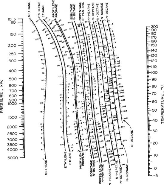
Note that T is in° R and p is in psia in Eq. (2-30). The constants a_T1, a_T2, a_T6, a_p1, a_p2, and a_p3 are given in Table 2-3. The last line gives the mean errors in the K values compared to the values from the DePriester charts. This equation is valid from −70° C (365.7° R) to 200° C (851.7° R) and for pressures from 101.3 kPa (14.69 psia) to 6000 kPa (870.1 psia). If K and p are known, then Eq. (2-30) can be solved for T. The obvious advantage of an equation compared to the charts is that it can be programmed into a computer or calculator. Equation (2-30) can be simplified for all components except n-octane and n-decane (see Eq. (6-15)).

Table 2-3. Constants for fit to K values using Eq. (2-30)

Note: T is in° R, and p is in psia

Source: McWilliams (1973)

The K values are used along with the stoichiometric equations which state the mole fractions in liquid and vapor phases must sum to 1.0.

(2-31)

where C is the number of components.

If only one component is present, then y = 1.0 and x = 1.0. This implies that K_i = y/x = 1.0. This gives a simple way of determining the boiling temperature of a pure compound at any pressure. For example, if we wish to find the boiling point of isobutane at p = 150 kPa, we set our straightedge on p = 150 and at 1.0 on the isobutane scale on Figure 2-11. Then read T = −1.5° C as the boiling point. Alternatively, Eq. (2-30) with values from Table 2-3 can be solved for T. This gives T = 488.68° R or −1.6° C.

For ideal systems Raoult’s law holds. Raoult’s law states that the partial pressure of a component is equal to its vapor pressure multiplied by its mole fraction in the liquid. Thus,

(2-32a)

where vapor pressure (VP) depends on temperature. By Dalton’s law of partial pressures,

(2-32b)

Combining these equations,

(2-32c)

Comparing Eqs. (2-32c) and (2-27), the Raoult’s law K value is

(2-33)

This is handy, since extensive tables of vapor pressures are available (e.g., Boublik et al., 1984; Perry and Green, 1997). Vapor pressure is often correlated in terms of the Antoine equation

(2-34)

Where A, B, and C are constants for each pure compound. These constants are tabulated in various data sources (Boublik et al., 1984; Yaws et al., 2005). The equations based on Raoult’s law should be used with great care, since deviations from Raoult’s law are extremely common.

Nonidealities in the liquid phase can be taken into account with a liquid-phase activity coefficient, γ_i. Then Eq. (2-33) becomes

(2-35)

The activity coefficient depends on temperature, pressure, and concentration. Excellent correlation procedures for activity coefficients such as the Margules, Van Laar, Wilson, NRTL, and UNIQUAC methods have been developed (Poling et al., 2001; Prausnitz et al., 1999; Sandler, 2006; Tester and Modell, 1997; Van Ness and Abbott, 1982; Walas, 1985). The coefficients for these equations for a wide variety of mixtures have been tabulated along with the experimental data (see Table 2-2). When the binary data are not available, one can use infinite dilution coefficients (Table 2-2; Carlson, 1996; Schad, 1998; Lazzaroni et al., 2005) or the UNIFAC group contribution method (Fredenslund et al., 1977; Prausnitz et al., 1980) to predict the missing data. Many distillation simulators use Eqs. (2-34), (2-35), and an appropriate activity coefficient equation. Although a detailed description of these methods is beyond the scope of this book, a guide to choosing VLE correlations for use in computer simulations is presented in Table 2-4.

Table 2-4. Approximate guides for selection of K-value methods.

Chemical Systems
Low MW Alcohol and Hydrocarbons		Wilson
Higher MW Alcohol and Hydrocarbons		NRTL
Hydrogen Bonding Systems		Margules
Liquid-Liquid Equilibrium		NRTL/UNIQUAC
Water as a Second Liquid Phase		NRTL
Components in a Homologous Family		UNIQUAC
Low Pressure Systems with Associating Vapor Phase		Hayden-O’Connell
Light Hydrocarbon and Oil Systems
Natural Gas Systems w/sweet and sour gas		SRK/PR
Cryogenic Systems		SRK/PR
Refinery Mixtures with p<5000 psia		SRK/PR
Hydrotreaters and Reformers		Grayson-Stread
Simple Paraffinic Systems		SRK/PR
Heavy Components w/ NBP>1,000°F		BK10
Aromatics (near critical region) + H2		PR/SRK
Based on Polarity and Ideality
nonpolar – nonpolar	ideal & non-ideal	any activity coefficient model
nonpolar – weakly polar	ideal	any activity coefficient model
nonpolar – weakly polar	non-ideal	UNIQUAC
nonpolar – strongly polar	ideal	UNIQUAC
nonpolar – strongly polar	non-ideal	Wilson
weakly polar – weakly polar	ideal	NRTL
weakly polar – weakly polar	non-ideal	UNIQUAC
weakly polar – strongly polar	ideal	NRTL
weakly polar – strongly polar	non-ideal	UNIQUAC
strongly polar – strongly polar	ideal	UNIQUAC
strongly polar – strongly polar	non-ideal	NO RECOMMENDATION
aqueous – strongly polar		UNIQUAC

Chemical systems and light hydrocarbon and oil systems suggestions courtesy of Dr. William Walters. Based on polarity and ideality suggestions from Gess et al. (1991) (see Table 2-2).

Key: NRTL = non-random two liquid model; SRK = Soave-Redlich-Kwong model; PR = Peng-Robinson; BK10 = Braun K10 for petroleum.

2.6 Multicomponent Flash Distillation

Equations (2-27) and (2-28) are solved along with the stoichiometric equations (2-31), the overall mass balance Eq. (2-5), the component mass balances,

(2-36)

and the energy balance, Eq. (2-7). Equation (2-36) is very similar to the binary mass balance, Eq. (2-6).

Usually the feed flow rate, F, and the feed mole fractions z_i for C − 1 of the components will be specified. If p_drum and T_drum or one liquid or vapor composition are also specified, then a sequential procedure can be used. That is, the mass balances, stoichiometric equations, and equilibrium equations are solved simultaneously, and then the energy balances are solved.

Now consider for a minute what this means. Suppose we have 10 components (C = 10). Then we must find 10 K’s, 10 x’s, one L, and one V, or 32 variables. To do this we must solve 32 equations [10 Eq. (2-27), 10 Eq. (2-31), and 10 independent mass balances, Eq. (2-36)] simultaneously. And this is the simpler sequential solution for a relatively simple problem.

How does one solve 32 simultaneous equations? In general, the K value relations could be nonlinear functions of composition. However, we will restrict ourselves to ideal solutions where Eq. (2-29) is valid and

K_i = K_i(T_drum, p_drum)

Since T_drum and p_drum are known, the 10 K_i can be determined easily [say, from the DePriester charts or Eq. (2-30)]. Now there are only 22 linear equations to solve simultaneously. This can be done, but trial-and-error procedures are simpler.

To simplify the solution procedure, we first use equilibrium, y_i = K_i x_i, to remove y_i from Eq. (2-36):

Fz_i = Lx_i + VK_i x_i i = 1, C

Solving for x_i, we have

If we solve Eq. (2-5) for L, L = F − V, and substitute this into the last equation we have

(2-37)

Now if the unknown V is determined, all of the x_i can be determined. It is usual to divide the numerator and denominator of Eq. (2-37) by the feed rate F and work in terms of the variable V/F. Then upon rearrangement we have

(2-38)

The reason for using V/F, the fraction vaporized, is that it is bounded between 0 and 1.0 for all possible problems. Since y_i = K_ix_i, we obtain

(2-39)

Once V/F is determined, x_i and y_i are easily found from Eqs. (2-38) and (2-39).

How can we derive an equation that allows us to calculate V/F?

To answer this, first consider what equations have not been used. These are the two stoichiometric equations, Σ x_i = 1.0 and Σ y_i = 1.0. If we substitute Eqs. (2-38) and (2-37) into these equations, we obtain

(2-40)

and

(2-41)

Either of these equations can be used to solve for V/F. If we clear fractions, these are Cth-order polynomials. Thus, if C is greater than 3, a trial-and-error procedure or root-finding technique must be used to find V/F. Although Eqs. (2-40) and (2-41) are both valid, they do not have good convergence properties. That is, if the wrong V/F is chosen, the V/F that is chosen next may not be better.

Fortunately, an equation that does have good convergence properties is easy to derive. To do this, subtract Eq. (2-40) from (2-41).

Subtracting the sums term by term, we have

(2-42)

Equation (2-42), which is known as the Rachford-Rice equation, has excellent convergence properties. It can also be modified for three-phase (liquid-liquid-vapor) flash systems (Chien, 1994).

Since the feed compositions, z_i, are specified and K_i can be calculated when T_drum and p_drum are given, the only variable in Eq. (2-42) is the fraction vaporized, V/F. This equation can be solved by many different convergence procedures or root finding methods. The Newtonian convergence procedure will converge quickly. Since f(V/F) in Eq. (2-42) is a function of V/F that should have a zero value, the equation for the Newtonian convergence procedure is

(2-43)

where f_k is the value of the function for trial k and df_k/d(V/F) is the value of the derivative of the function for trial k. We desire to have f_{k + 1} equal zero, so we set f_{k + 1} = 0 and solve for Δ (V/F):

(2-44)

This equation gives us the best next guess for the fraction vaporized. To use it, however, we need equations for both the function and the derivative. For f_k, use the Rachford-Rice equation, (2-42). Then the derivative is

(2-45)

Substituting Eqs. (2-42) and (2-45) into (2-44) and solving for (V/F)_k+1, we obtain

(2-46)

Equation (2-46) gives a good estimate for the next trial. Once (V/F)_k+1 is calculated the value of the Rachford-Rice function can be determined. If it is close enough to zero, the calculation is finished; otherwise repeat the Newtonian convergence for the next trial.

Newtonian convergence procedures do not always converge. One advantage of using the Rachford-Rice equation with the Newtonian convergence procedure is that there is always rapid convergence. This is illustrated in Example 2-2.

Once V/F has been found, x_i and y_i are calculated from Eqs. (2-38) and (2-39). L and V are determined from the overall mass balance, Eq. (2-5). The enthalpies h_L and H_v can now be calculated. For ideal solutions the enthalpies can be determined from the sum of the pure component enthalpies multiplied by the corresponding mole fractions:

(2-47)

(2-48)

where and are enthalpies of the pure components. If the solutions are not ideal, heats of mixing are required. Then the energy balance, Eq. (2-7), is solved for h_F, and T_F is determined.

If V/F and p_drum are specified, then T_drum must be determined. This can be done by picking a value for T_drum, calculating K_i, and checking with the Rachford-Rice equation, (2-42). A plot of f(V/F) vs. T_drum will help us select the temperature value for the next trial. Alternatively, an approximate convergence procedure similar to that employed for bubble- and dew-point calculations can be used (see Section 6.3). The new K_ref can be determined from

(2-49)

where the damping factor d ≤ 1.0. In some cases this may overcorrect unless the initial guess is close to the correct answer. The calculation when V/F = 0 gives us the bubble point temperature (liquid starts to boil) and when V/F = 1.0 gives the dew point temperature (vapor starts to condense).

Example2-2. Multicomponent flash distillation

A flash chamber operating at 50° C and 200 kPa is separating 1,000 kg moles/hr of a feed that is 30 mole % propane, 10 mole % n-butane, 15 mole % n-pentane and 45 mole % n-hexane. Find the product compositions and flow rates.

Solution

A. Define. We want to calculate y_i, x_i, V, and L for the equilibrium flash chamber shown in the diagram.

B. Explore. Since T_drum and p_drum are given, a sequential solution can be used. We can use the Rachford-Rice equation to solve for V/F and then find x_i, y_i, L, and V.

C. Plan. Calculate K_i from DePriester charts or from Eq. (2-30). Use Newtonian convergence with the Rachford-Rice equation, Eq. (2-46), to converge on the correct V/F value. Once the correct V/F has been found, calculate x_i from Eq. (2-38) and y_i from Eq. (2-39). Calculate V from V/F and L from overall mass balance, Eq. (2-5).

D. Do it. From the DePriester chart (Fig.2-11), at 50° C and 200 kPa we find

K1 = 7.0	C3
K2 = 2.4	n-C4
K3 = 0.80	n-C5
K4 = 0.30	n-C6

Calculate f (V/F) from the Rachford-Rice equation:

Pick V/F = 0.1 as first guess (this illustrates convergence for a poor first guess).

Since f(0.1) is positive, a higher value for V/F is required. Note that only one term in the denominator of each term changes. Thus we can set up the equation so that only V/F will change. Then f(V/F) equals

Now all subsequent calculations will be easier.

The derivative of the R-R equation can be calculated for this first guess

With V/F = 0.1 this is = −4.631

From Eq. (2-46) the next guess for V/F is (V/F)₂ = 0.1 + 0.8785/4.631 = 0.29. Calculating the value of the Rachford-Rice equation, we have f(0.29) = 0.329. This is still positive and V/F is still too low.

Second Trial:

which gives (V/F)₃ = 0.29 + 0.329/1.891 = 0.46

and the Rachford-Rice equation is f(0.46) = 0.066. This is closer, but V/F is still too low. Continue convergence.

Third Trial:

which gives (V/F)₄ = 0.46 + 0.066/1.32 = 0.51

We calculate that f(0.51) = 0.00173 which is very close and is within the accuracy of the DePriester charts. Thus V/F = 0.51.

Now we calculate x_i from Eq. (2-38) and y_i from K_ix_i,

By similar calculations,	x2 = 0.0583,	y2 = 0.1400
	x3 = 0.1670,	y3 = 0.1336
	x4 = 0.6998,	y4 = 0.2099

Since F = 1,000 and V/F = 0.51, V = 0.51F = 510 kg moles/hr, and L = F − V = 1,000 − 510 = 490 kg moles/hr.

E. Check. We can check Σ y_i and Σ x_i.

These are close enough. They aren’t perfect, because V/F wasn’t exact. Essentially the same answer is obtained if Eq. (2-30) is used for the K values. Note: Equation (2-30) may seem more accurate since one can produce a lot of digits; however, since it is a fit to the DePriester chart it can’t be more accurate.

F. Generalize. Since the Rachford-Rice equation is almost linear, the Newtonian convergence routine gives rapid convergence. Note that the convergence was monotonic and did not oscillate. Faster convergence would be achieved with a better first guess of V/F. This type of trial-and-error problem is easy to program on a spreadsheet.

If the specified variables are F, z_i, p_drum, and either x or y for one component, we can follow a sequential convergence procedure using Eq. (2-38) or (2-39) to relate to the specified composition (the reference component) to either K_ref or V/F. We can do this in either of two ways. The first is to guess T_drum and use Eq. (2-38) or (2-39) to solve for V/F. The Rachford-Rice equation is then the check equation on T_drum. If the Rachford-Rice equation is not satisfied we select a new temperature—using Eq. (2-49)—and repeat the procedure. In the second approach, we guess V/F and calculate K_ref from Eq. (2-38) or (2-39). We then determine the drum temperature from this K_ref. The Rachford-Rice equation is again the check. If it is not satisfied, we select a new V/F and continue the process.

2.7 Simultaneous Multicomponent Convergence

If the feed rate F, the feed composition consisting of (C − 1) z_i values, the flash drum pressure p_drum, and the feed temperature T_F are specified, the hot liquid will vaporize when its pressure is dropped. This “flashing” cools the liquid to provide energy to vaporize some of the liquid. The result T_drum is unknown; thus, we must use a simultaneous solution procedure. First, we choose a feed pressure such that the feed will be liquid. Then we can calculate the feed enthalpy in the same way as Eqs. (2-47) and (2-48):

(2-50)

Although the mass and energy balances, equilibrium relations, and stoichiometric relations could all be solved simultaneously, it is again easier to use a trial-and-error procedure. This problem is now a double trial-and-error.

The first question to ask in setting up a trial-and-error procedure is: What are the possible trial variables and which ones shall we use? Here we first pick T_drum, since it is required to calculate all K_i, and and since it is difficult to solve for. The second trial variable is V/F, because then we can use the Rachford-Rice approach with Newtonian convergence.

The second question to ask is: Should we converge on both variables simultaneously (that is change both T_drum and V/F at the same time), or should we converge sequentially? Both techniques will work, but, if applied properly, sequential convergence tends to be more stable. If we use sequential convergence, then a third question is: Which variable should we converge on first, V/F or T_drum? To answer this question we need to consider the chemical system we are separating. If the mixture is wide-boiling, that is, if the dew point and bubble point are far apart (say more than 80 to 100° C), then a small change in T_drum cannot have much effect on V/F. In this case we wish to converge on V/F first. Then when T_drum is changed, we will be close to the correct answer for V/F. For a significant separation in a flash system, the volatilities must be very different, so this is the typical situation for flash distillation. The narrow-boiling procedure is shown in Figure 6-1 for distillation.

The procedure for wide-boiling feeds is shown in Figure 2-13. Note that the energy balance is used last. This is standard procedure since accurate values of x_i and y_i are available to calculate enthalpies for the energy balance.

Figure 2-13. Flowsheet for wide-boiling feed

The fourth question is: How should we do the individual convergence steps? For the Rachford-Rice equation, linear interpolation or Newtonian convergence will be satisfactory. Several methods can be used to estimate the next flash drum temperature. One of the fastest and easiest to use is a Newtonian convergence procedure. To do this we rearrange the energy balance (Eq. 2-7) into the functional form,

(2-51)

The subscript k again refers to the trial number. When E_k is zero, the problem has been solved. The Newtonian procedure estimates E_k+1(T_drum) from the derivative,

(2-52)

where ΔT_drum is the change in T_drum from trial to trial,

(2-53)

and dE_k/dT_drum is the variation of E_k as temperature changes. Since the last two terms in Eq. (2-51) do not depend on T_drum, this derivative can be calculated as

(2-54)

where we have used the definition of the heat capacity. In deriving Eq. (2-54) we set both dV/dT and dL/dT equal to zero since a sequential convergence routine is being used and we do not want to vary V and L in this loop. We want the energy balance to be satisfied after the next trial. Thus we set E_k+1 = 0. Now Eq. (2-52) can be solved for ΔT_drum:

(2-55)

Substituting the expression for ΔT_drum into this equation and solving for T_{drum k+1}, we obtain the best guess for temperature for the next trial,

(2-56)

In this equation E_k is the calculated numerical value of the energy balance function from Eq. (2-51) and dE_k/dT_drum is the numerical value of the derivative calculated from Eq. (2-54).

The procedure has converged when

(2-56a)

For computer calculations, ε = 0.01° C is a reasonable choice. For hand calculations, a less stringent limit such as ε = 0.2° C would be used. This procedure is illustrated in Example 2-3.

It is possible that this convergence scheme will predict values of ΔT_drum that are too large. When this occurs, the drum temperature may oscillate with a growing amplitude and not converge. To discourage this behavior, ΔT_drum can be damped.

(2-57)

where the damping factor d is about 0.5. Note that when d = 1.0 this is just the Newtonian approach.

The drum temperature should always lie between the bubble- and dew-point temperature of the feed. In addition, the temperature should converge toward some central value. If either of these criteria is violated, then the convergence scheme should be damped or an alternative convergence scheme should be used.

Example 2-3. Simultaneous convergence for flash distillation

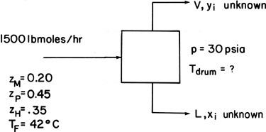
We have a liquid feed that is 20 mole % methane, 45 mole % n-pentane, and 35 mole % n-hexane. Feed rate is 1500 kg moles/hr, and feed temperature is 45° C and pressure is 100.0 psia. The flash drum operates at 30 psia and is adiabatic. Find: T_drum, V/F, x_i, y_i, L, V.

Solution

A. Define. The process is sketched in the diagram.

B. Explore. Since T_F is given, this will be a double trial and error. K values from the DePriester charts or from Eq. (2-30) can be used. For energy balances, enthalpies can be calculated from heat capacities and latent heats. The required data are listed in Table 2-5.

C. Plan. Since this is a double trial and error, all calculations will be done on the computer and summarized here. Newtonian convergence will be used for both the Rachford-Rice equation and the energy balance estimate of new drum temperature. ε = 0.02 is used for energy convergence (Eq. 2-56). The Rachford-Rice equation is considered converged when

(2-58)

ε_R = 0.005 is used here.

D. Do It. The first guess is made by arbitrarily assuming that T_drum = 15° C and V/F = 0.25. Since convergence of the program is rapid, more effort on an accurate first guess is probably not justified. Using Eq. (2-46) as illustrated in Example 2-2, the following V/F values are obtained [K values from Eq. (2-30)]:

V/F =	0.25, 0.2485, 0.2470, 0.2457, 0.2445, 0.2434, 0.2424, 0.2414, 0.2405,
	0.2397, 0.2390, 0.2383, 0.2377, 0.2371, 0.2366, 0.2361

Table 2-5 Data for methane, n-pentane, and n-hexane

Himmelblau (1974)

Note that convergence is monotonic. With V/F known, x_i and y_i are found from Eqs. (2-38) and (2-39).

Compositions are: x_m = 0.0124, x_p = 0.5459, x_H = 0.4470, and y_m = 0.8072, y_p = 0.1398, y_H = 0.0362.

Flow rates L and V are found from the mass balance and V/F value. After determining enthalpies, Eq. (2-56) is used to determine T_drum,2 = 27.9° C. Obviously, this is still far from convergence.

The convergence procedure is continued, as summarized in Table 2-6. Note that the drum temperature oscillates, and because of this the converged V/F oscillates. Also, the number of trials to converge on V/F decreases as the calculation proceeds. The final compositions and flow rates are:

x_m = 0.0108, x_p = 0.5381, x_H = 0.4513

y_m = 0.7531, y_P = 0.1925, y_H = 0.0539

V = 382.3 kg-mole/hr and L = 1117.7 kg-mole/hr

Table 2-6 Iterations for Example 2-3

E. Check. The results are checked throughout the trial-and-error procedure. Naturally, they depend upon the validity of data used for the enthalpies and Ks. At least the results appear to be self-consistent (that is, Σ x_i = 1.0, Σ y_i = 1.0) and are of the right order of magnitude. This problem was also solved using Aspen Plus with the Peng-Robinson equation for VLE (see Chapter 2 Appendix). The results are x_m = 0.0079, x_p = 0.5374, x_H = 0.4547, L = 1107.8, and y_m = 0.7424, y_p = 0.2032, y_H = 0.0543, V = 392.2, and T_drum = 27.99° C. With the exception of the drum temperature these results, which use different data, are close.

F. Generalization. The use of the computer greatly reduces calculation time on this double trial-and-error problem. Use of a process simulator that includes VLE and enthalpy correlations will be fastest.

2.8 Size Calculation

Once the vapor and liquid compositions and flow rates have been determined, the flash drum can be sized. This is an empirical procedure. We will discuss the specific procedure first for vertical flash drums (Figure 2-1) and then adjust the procedure for horizontal flash drums.

Step 1. Calculate the permissible vapor velocity, u_perm,

(2-59)

u_perm is the maximum permissible vapor velocity in feet per second at the maximum cross-sectional area. ρ_L and ρ_v are the liquid and vapor densities.

K_drum is an empirical constant that depends on the type of drum. For vertical drums the value has been correlated graphically by Watkins (1967) for 85% of flood with no demister. Approximately 5% liquid will be entrained with the vapor. Use of the same design with a demister will reduce entrainment to less than 1%. The demister traps small liquid droplets on fine wires and prevents them from exiting. The droplets then coalesce into larger droplets, which fall off the wire and through the rising vapor into the liquid pool at the bottom of the flash chamber. Blackwell (1984) fit Watkins’ correlation to the equation

(2-60)

where

with W_L and W_v being the liquid and vapor flow rates in weight units per hour (e.g., lb/hr). The constants are (Blackwell, 1984):

A = −1.877478097	C = −0.1870744085	E = −0.0010148518
B = −0.8145804597	D = −0.0145228667

The resulting value for K_drum typically ranges from 0.1 to 0.35.

Step 2. Using the known vapor rate, V, convert u_perm into a horizontal area. The vapor flow rate, V, in lb moles/hr is

Solving for the cross-sectional area,

(2-61)

For a vertical drum, diameter D is

(2-62)

Usually, the diameter is increased to the next largest 6-in. increment.

Step 3. Set the diameter/length ratio either by rule of thumb or by the required liquid surge volume. For vertical flash drums, the rule of thumb is that L/D ranges from 3.0 to 5.0. The appropriate value of L/D within this range can be found by minimizing the total vessel weight (which minimizes cost).

Flash drums are often used as liquid surge tanks in addition to separating liquid and vapor. The design procedure for this case is discussed by Watkins (1967) for petrochemical applications.

The height of the drum above the centerline of the feed nozzle, h_v, should be 36 in. plus one-half the diameter of the feed line (see Figure 2-14). The minimum of this distance is 48 in.

Figure 2-14 Measurements for vertical flash drum

The height of the center of the feed line above the maximum level of the liquid pool, h_f, should be 12 in. plus one-half the diameter of the feed line. The minimum distance for this free space is 18 in.

The depth of the liquid pool, h_L, can be determined from the desired surge volume, V_surge.

(2-63)

The geometry can now be checked, since

should be between 3 and 5. These procedures are illustrated in Example 2-4. If h_total/D < 3, a larger liquid surge volume should be allowed. If h_total/D > 5, a horizontal flash drum should be used. Calculator programs for sizing both vertical and horizontal drums are available (Blackwell, 1984).

For horizontal drums Blackwell (1984) recommends using

(2-64a)

Calculate A_c from Eq. (2-61) and empirically determine the total cross sectional area A_T as,

(2-64b)

and then the diameter of the horizontal drum is,

(2-58)

The typical range for h_total/D is from 3 to 5. Horizontal drums are particularly useful when large liquid surge capacities are needed. More detailed design procedures and methods for horizontal drums are presented by Evans (1980), Blackwell (1984), and Watkins (1967). Note that in industries other than petrochemicals that sizing may vary.

Example 2-4. Calculation of drum size

A vertical flash drum is to flash a liquid feed of 1500 lb moles/hr that is 40 mole % n-hexane and 60 mole % n-octane at 101.3 kPa (1 atm). We wish to produce a vapor that is 60 mole % n-hexane. Solution of the flash equations with equilibrium data gives x_H = 0.19, T_drum = 378K, and V/F = 0.51. What size flash drum is required?

Solution

A. Define. We wish to find diameter and length of flash drum.

B. Explore. We want to use the empirical method developed in Eqs. (2-59) to (2-63). For this we need to estimate the following physical properties: ρ_L, ρ_v, MW_v. To do this we need to know something about the behavior of the gas and of the liquid.

C. Plan. Assume ideal gas and ideal mixtures for liquid. Calculate average ρ_L by assuming additive volumes. Calculate ρ_v from the ideal gas law. Then calculate u_perm from Eq. (2-59) and diameter from Eq. (2-63).

D. Do It.

1. Liquid Density

The average liquid molecular weight is

where subscript H is n-hexane and O is n-octane. Calculate or look up the molecular weights. MW_H = 86.17 and MW_O = 114.22. Then . The specific volume is the sum of mole fractions multiplied by the pure component specific volumes (ideal mixture):

From the Handbook of Chemistry and Physics, ρ_H = 0.659 g/mL and ρ_O = 0.703 g/mL at 20° C. Thus,

Then

2. Vapor Density

Density in moles per liter for ideal gas is _v = n/V = p/RT, which in grams per liter is.

The average molecular weight of the vapor is

where y_H = 0.60 and y_O = 0.40, and thus . This gives

3. K_drum Calculation.

Calculation of flow parameter F_lv:

V = (V/F)(F) = (0.51)(1500) = 765 lb moles/hr

L = F − V = 735 lb moles/hr

K_drum from Eq. (2-60) gives K_drum = 0.4433, which seems a bit high but agrees with Watkin’s (1967) chart.

4.

5.

Use a 4.0 ft diameter drum or 4.5 ft to be safe.

6. If use h_total/D = 4, h_total = 4(4.5 ft) = 18.0 ft.

E. Check. This drum size is reasonable. Minimums for h_v and h_f are easily met. Note that units do work out in all calculations; however, one must be careful with units, particularly calculating A_c and D.

F. Generalization. If the ideal gas law is not valid, a compressibility factor could be inserted in the equation for ρ_v. Note that most of the work involved calculation of the physical properties. This is often true in designing equipment. In practice we pick a standard size drum (4.0 or 4.5 ft diameter) instead of custom building the drum.

2.9 Using Existing Flash Drums

Individual pieces of equipment will often outlive the entire plant. This used equipment is then available either in the plant’s salvage section or from used equipment dealers. As long as used equipment is clean and structurally sound (it pays to have an expert check it), it can be used instead of designing and building new equipment. Used equipment and off-the-shelf new equipment will often be cheaper and will have faster delivery than custom-designed new equipment; however, it may have been designed for a different separation. The challenge in using existing equipment is to adapt it with minimum cost to the new separation problem.

The existing flash drum has its dimensions h_total and D specified. Solving Eqs. (2-61) and (2-62) for a vertical drum for V, we have

(2-65)

This vapor velocity is the maximum for this existing drum, since it will give a linear vapor velocity equal to u_perm.

The maximum vapor capacity of the drum limits the product of (V/F) multiplied by F, since we must have

(2-66)

If Eq. (2-66) is satisfied, then use of the drum is straightforward. If Eq. (2-66) is violated, something has to give. Some of the possible adjustments are:

a. Add chevrons or a demister to increase V_Max or to reduce entrainment (Woinsky, 1994).

b. Reduce feed rate to the drum.

c. Reduce V/F. Less vapor product with more of the more volatile components will be produced.

d. Use existing drums in parallel. This reduces feed rate to each drum.

e. Use existing drums in series (see Problems 2.D2 and 2.D5).

f. Try increasing the pressure (note that this changes everything—see Problem 2.C1).

g. Buy a different flash drum or build a new one.

h. Use some combination of these alternatives.

i. The engineer can use ingenuity to solve the problem in the cheapest and quickest way.

2.10 Summary—Objectives

This chapter has discussed VLE and the calculation procedures for binary and multicomponent flash distillation. At this point you should be able to satisfy the following objectives:

1. Explain and sketch the basic flash distillation process

2. Find desired VLE data in the literature or on the Web

3. Plot and use y-x, temperature-composition, enthalpy-composition diagrams; explain the relationship between these three types of diagrams

4. Derive and plot the operating equation for a binary flash distillation on a y-x diagram; solve both sequential and simultaneous binary flash distillation problems

5. Define and use K values, Raoult’s law, and relative volatility

6. Derive the Rachford-Rice equation for multicomponent flash distillation, and use it with Newtonian convergence to determine V/F

7. Solve sequential multicomponent flash distillation problems

8. Determine the length and diameter of a flash drum

9. Use existing flash drums for a new separation problem

References

Barnicki, S. D., “How Good are Your Data?” Chem. Engr. Progress,98 (6), 58 (June 2002).

Blackwell, W. W., Chemical Process Design on a Programmable Calculator, McGraw-Hill, New York, 1984, chapter 3.

Boublik, T., V. Fried, and E. Hala, Vapour Pressures of Pure Substances, Elsevier, Amsterdam, 1984.

Carlson, E. C., “Don’t Gamble with Physical Properties for Simulators,” Chem. Engr. Progress, 92(10), 35 (Oct. 1996).

Chien, H. H.-y., “Formulations for Three-Phase Flash Calculations,” AIChE Journal, 40(6), 957 (1994).

Dadyburjor, D. B., “SI Units for Distribution Coefficients,” Chem. Engr. Progress, 74(4), 85 (April 1978).

Evans, F. L., Jr., Equipment Design Handbook for Refineries and Chemical Plants, Vol. 2, 2^nd ed., Gulf Publishing Co., Houston, TX, 1980.

Fredenslund, A., J. Gmehling and P. Rasmussen, Vapor-Liquid Equilibria Using UNIFAC: A Group-Contribution Method, Elsevier, Amsterdam, 1977.

Himmelblau, D. M., Basic Principles and Calculations in Chemical Engineering, 3^rd ed, Prentice-Hall, Upper Saddle River, NJ, 1974.

King, C. J., Separation Processes, 2^nd ed., McGraw-Hill, New York, 1981.

Lazzaroni, M. J., D. Bush, C. A. Eckert, T. C. Frank, S. Gupta and J. D. Olsen, “Revision of MOSCED Parameters and Extension to Solid Solubility Calculations,” Ind. Eng. Chem. Research, 44, 4075 (2005).

Maxwell, J. B., Data Book on Hydrocarbons, Van Nostrand, Princeton, NJ, 1950.

McWilliams, M. L., “An Equation to Relate K-factors to Pressure and Temperature,” Chem. Engineering, 80(25), 138 (Oct. 29, 1973).

Marsh, K. N., “The Measurement of Thermodynamic Excess Functions of Binary Liquid Mixtures,” Chemical Thermodynamics, Vol. 2, The Chemical Society, London, 1978, pp. 1-45.

Nelson, A. R., J. H. Olson, and S. I. Sandler, “Sensitivity of Distillation Process Design and Operation to VLE Data,” Ind. Eng. Chem. Process Des. Develop., 22, 547 (1983).

Perry, R. H., C. H. Chilton and S. D. Kirkpatrick (Eds.), Chemical Engineer’s Handbook, 4^th ed., McGraw-Hill, New York, 1981.

Perry, R. H. and D. Green (Eds.), Perry’s Chemical Engineer’s Handbook, 7^th ed., McGraw-Hill, New York, 1997.

Poling, B. E., J. M. Prausnitz and J. P. O’Connell, The Properties of Gases and Liquids, 5^th ed., McGraw-Hill, New York, 2001.

Prausnitz, J. M., T. F. Anderson, E. A. Grens, C. A. Eckert, R. Hsieh and J. P. O’Connell, Computer Calculations for Multicomponent Vapor-Liquid and Liquid-Liquid Equilibria, Prentice-Hall, Upper Saddle River, NJ, 1980.

Prausnitz, J. M., R. N. Lichtenthaler and E. G. de Azevedo, Molecular Thermodynamics of Fluid-Phase Equilibria, 3^rd ed., Prentice-Hall, Upper Saddle River, NJ, 1999.

Sandler, S. I., Chemical and Engineering Thermodynamics, 4^th ed., Wiley, New York, 2006.

Schad, R. C., “Make the Most of Process Simulation,” Chem. Engr. Progress, 94(1), 21 (Jan. 1998).

Seider, W. D., J. D. Seader and D. R. Lewin, Process Design Principles, Wiley, New York, 1999.

Smith, B. D., Design of Equilibrium Stage Processes, McGraw-Hill, New York, 1963.

Smith, J. M., H. C. Van Ness and M. M. Abbott, Introduction to Chemical Engineering Thermodynamics, 7^th ed., McGraw-Hill, New York, 2005.

Tester, J. W. and M. Modell, Thermodynamics and Its Applications, 3^rd ed., Prentice Hall PTR, Upper Saddle River, NJ 1997.

Van Ness, H. C. and M. M. Abbott, Classical Thermodynamics of Non-Electrolyte Solutions. With Applications to Phase Equilibria, McGraw-Hill, New York, 1982.

Walas, S. M., Phase Equilibria in Chemical Engineering, Butterworth, Boston, 1985.

Wankat, P. C., Equilibrium-Staged Separations, Prentice-Hall, Upper Saddle River, NJ, 1988.

Woinsky, S. G., “Help Cut Pollution with Vapor/Liquid and Liquid/Liquid Separators,” Chem. Engr. Progress, 90(10), 55 (Oct. 1994).

Yaws, C. L., P. K. Narasimhan and C. Gabbula, Yaw’s Handbook of Antoine Coefficients for Vapor Pressure (Electronic Edition), Knovel, 2005.

Homework

A. Discussion Problems

A1. In Figure 2-9 the feed plots as a two-phase mixture, whereas it is a liquid before introduction to the flash chamber. Explain why. Why can’t the feed location be plotted directly from known values of T_F and z? In other words, why does h_F have to be calculated separately from an equation such as Eq. (2-9b)?

A2. Can weight units be used in the flash calculations instead of molar units?

A3. Explain why a sequential solution procedure cannot be used when T_feed is specified for a flash drum.

A4. In the flash distillation of salt water, the salt is totally nonvolatile (this is the equilibrium statement). Show a McCabe-Thiele diagram for a feed water containing 3.5 wt % salt. Be sure to plot weight fraction of more volatile component.

A5. Develop your own key relations chart for this chapter. That is, on one page summarize everything you would want to know to solve problems in flash distillation. Include sketches, equations, and key words.

A6. Pressure has significant effects on flash drums. If the drum pressure is increased,

a. what happens to drum temperature (assume y is fixed)?

b. is more or less separation achieved?

c. is the drum diameter larger or smaller?

A7. a. What would Figure 2-2 look like if we plotted y₂ vs. x₂ (i.e., plot less volatile component mole fractions)?

b. What would Figure 2-3 look like if we plotted T vs. x₂ or y₂ (less volatile component)?

c. What would Figure 2-4 look like if we plotted H or h vs. y₂ or x₂ (less volatile component)?

A8. For a typical straight-chain hydrocarbon, does:

a. K increase, decrease, or stay the same when temperature is increased?

b. K increase, decrease, or stay the same when pressure is increased?

c. K increase, decrease, or stay the same when mole fraction in the liquid phase is increased?

d. K increase, decrease, or stay the same when the molecular weight of the hydrocarbon is increased within a homologous series?

Note: It will help to visualize the DePreister chart in answering this question.

A9. Why do the values of the azeotrope composition appear to be different in Figures 2-3 and 2-4

A10. At what temperature does pure propane boil at 700 kPa?

B. Generation of Alternatives

B1 Think of all the ways a binary flash distillation problem can be specified. For example, we have usually specified F, z, T_drum, p_drum. What other combinations of variables can be used? (I have over 20.) Then consider how you would solve the resulting problems.

B2. An existing flash drum is available. The vertical drum has a demister and is 4 ft in diameter and 12 ft tall. The feed is 30 mole % methanol and 70 mole % water. A vapor product that is 58 mole % methanol is desired. We have a feed rate of 25,000 lb moles/hr. Operation is at 1 atm pressure. Since this feed rate is too high for the existing drum, what can be done to produce a vapor of the desired composition? Design the new equipment for your new scheme. You should devise at least three alternatives. Data are given in Problem 2.D1.

B3. In principle, measuring VLE data is straightforward. In practice, actual measurement may be very difficult. Think of how you might do this. How would you take samples without perturbing the system? How would you analyze for the concentrations? What could go wrong? Look in your thermodynamics textbook for ideas.

C. Derivations

C1. Determine the effect of pressure on the temperature, separation and diameter of a flash drum.

C2. Solve the Rachford-Rice equation for V/F for a binary system.

C3. Assume that vapor pressure can be calculated from the Antoine equation and that Raoult’s law can be used to calculate K values. For a binary flash system, solve for the drum pressure if drum temperature and V/F are given.

C4. Convert Eqs. (2-60) and (2-61) to SI units.

C5. Choosing to use V/F to develop the Rachford-Rice equation is conventional but arbitrary. We could also use L/F, the fraction remaining liquid, as the trial variable. Develop the Rachford-Rice equation as f(L/F).

C6. In flash distillation a liquid mixture is partially vaporized. We could also take a vapor mixture and partially combine it. Draw a schematic diagram of partial condensation equipment. Derive the equations for this process. Are they different from flash distillation? If so, how?

C7. Plot Eq. (2-40) vs. V/F for Example 2-2 to illustrate that convergence is not as linear as the Rachford-Rice equation.

D. Problems

*Answers to problems with an asterisk are at the back of the book.

D1. * We are separating a mixture of methanol and water in a flash drum at 1 atm pressure. Equilibrium data are listed in Table 2-7.

a. Feed is 60 mole % methanol, and 40 % of the feed is vaporized. What are the vapor and liquid mole fractions and flow rates? Feed rate is 100 kg moles/hr.

b. Repeat part A for a feed rate of 1500 kg moles/hr.

c. If the feed is 30 mole % methanol and we desire a liquid product that is 20 mole % methanol, what V/F must be used? For a feed rate of 1,000 lb moles/hr, find product flow rates and compositions.

d. We are operating the flash drum so that the liquid mole fraction is 45 mole % methanol. L = 1500 kg moles/hr, and V/F = 0.2. What must the flow rate and composition of the feed be?

e. Find the dimensions of a vertical flash drum for Problem D-1c.

Table2-7 Vapor-Liquid Equilibrium Data for Methanol Water (p = 1 atm)

Source: Perry et al. (1963), p. 13–5.

Data: ρ_w = 1.00 g/cm³, ρ_m,L = 0.7914 g/cm³, MW_w = 18.01, MW_m = 32.04. Assume vapors are ideal gas.

f. If z = 0.4, p = 1 atm, and T_drum = 77° C, find V/F, x_m, and y_m.

D2. * Two flash distillation chambers are hooked together as shown in the diagram. Both are at 1 atm pressure. The feed to the first drum is a binary mixture of methanol and water that is 55 mole % methanol. Feed flow rate is 10,000 kg moles/hr. The second flash drum operates with (V/F)₂ = 0.7 and the liquid product composition is 25 mole % methanol. Equilibrium data are given in Table 2-7.

a. What is the fraction vaporized in the first flash drum?

b. What are y₁, y₂, x₁, T₁, and T₂?

D3. We are separating a mixture of methanol and water in a flash drum at 1.0 atm pressure. Use the equilibrium data listed in Table 2-7. Feed rate is 10.0 kmole/hr.

a. The feed is 40 mole % methanol and 60% of the feed is vaporized. Find mole fractions and flow rates of vapor and liquid products. Estimate the temperatures by linear interpolation for both vapor and liquid products.

b. The feed is 40 mole % methanol, the product temperatures are both 78.0°C. Find the mole fractions of liquid and vapor products and V/F.

c. We desire a vapor product that is 80 mole % methanol and want to operate at V/F = 0.3. What must the feed composition be?

D4. 100.0 kmoles/day of a feed that is 10 mole % ethane, 35 mole % n-pentane and 55 mole % n-heptane is fed to a flash drum. The drum pressure is 1,000 kPa and the drum temperature is 120°C. Find V/F, x_i and y_i. Use DePriester chart.

D5. We have a feed that is a binary mixture of methanol and water (55.0 mole % methanol) that is sent to a system of two flash drums hooked together. The vapor from the first drum is cooled, which partially condenses the vapor, and then is fed to the second flash drum. Both drums operate at a pressure of 1.0 atm and are adiabatic. The feed rate to the first drum is 1,000 kmoles/hr. We desire a liquid product from the first drum that is 30.0 mole % methanol (x₁ = 0.30). The second drum operates at a fraction vaporized of (V/F)₂ = 0.25. The equilibrium diagram is in Table 2-7.

a. Sketch the process labeling the different streams.

b. Find the following for the first drum: vapor mole fraction y₁, fraction vaporized (V/F)₁, and vapor flow rate V₁.

c. Find the following for the second drum: vapor mole fraction y₂, liquid mole fraction x₂, and vapor flow rate V₂.

D6. A feed that is 45.0 mole % n-butane, 35.0 mole % n-pentane, and 20.0 mole % n-hexane is fed at a rate of 1.0 kmoles/min to a flash drum operating at 50°C and 200 kPa. Find V/F, liquid mole fractions and vapor mole fractions. Use the DePriester charts.

D7. A flash drum is separating methane from propane at 0°C and 2500 kPa. The feed is 30.0 mole % methane and 70.0 mole % propane. Find V/F, y and x. Use the results of problem 2.C2. Use the DePriester chart for K values.

D8. *You want to flash a mixture with a drum pressure of 2 atm and a drum temperature of 25° C. The feed is 2000 kg moles/hr. The feed is 5 mole % methane, 10 mole % propane, and the rest n-hexane. Find the fraction vaporized, vapor mole fractions, liquid mole fractions, and vapor and liquid flow rates. Use DePriester charts.

D9. *We wish to flash distill an ethanol-water mixture that is 30 wt % ethanol and has a feed flow of 1,000 kg/hr. Feed is at 200° C. The flash drum operates at a pressure of 1 kg/cm². Find: T_drum, wt frac of liquid and vapor products, and liquid and vapor flow rates.

Data:

C_PL,EtOH = 37.96 at 100° C, kcal/kg mole° C

C_PL,W = 18.0, kcal/kg mole° C

C_PV,EtOH = 14.66 + 3.758 × 10⁻²T − 2.091 × 10⁻⁵T² + 4.74 × 10⁻⁹T³

C_PV,W = 7.88 + 0.32 × 10⁻²T−0.04833 × 10⁻⁵T²

Both C_PV values are in kcal/kg mole° C, with T in° C.

ρ_EtOH = 0.789 g/mL, ρ_W = 1.0 g/mL, MW_EtOH = 46.07, MW_W = 18.016, λ_EtOH = 9.22 kcal/g mole at 351.7 K, and λ_W = 9.7171 kcal/g mole at 373.16 K.

Enthalpy composition diagram at p = 1 kg/cm² is in Figure 2-4. Note: Be careful with units.

D10. A mixture that is 25 mole % benzene and 75 mole % toluene is flashed. Feed is 200 kmoles/hr. The liquid product is 15 mole % benzene. The constant relative volatility is = 2.4. Find y and L. Do this problem analytically, not graphically.

D11. A vapor stream which is 40.0 mole % ethanol and 60.0 mole % water is partially condensed and sent to a flash drum operating at 1.0 atm.

a. What is the highest vapor mole fraction which can be produced?

b. If 60.0 % of the feed is liquefied, what are the outlet mole fractions of liquid and vapor?

D12. Find the dimensions (h_total and D) for a horizontal flash drum for Problem 2.D1c. Use h_total/D = 4.

D13. *A flash drum is to flash 10,000 lb moles/hr of a feed that is 65 mole % n-hexane and 35 mole % n-octane at 1 atm pressure. V/F = 0.4.

a. Find T_drum, liquid mole fraction, vapor mole fraction.

b. Find the size required for a vertical flash drum.

Note, y, x, T equilibrium data can be determined from the DePriester charts. Other required physical property data are given in Example 2-4.

D14. We are feeding 100 kgmoles/hr of a mixture that is 30 mole % n-butane and 70 mole % n-hexane to a flash drum. We operate with V/F = 0.4 and T_drum = 100°C. Use Raoult’s law to estimate K values from vapor pressures. Use Antoine’s equation to calculate vapor pressure,

where VP is in mm Hg and T is in°C.

n-butane: A = 6.809, B = 935.86, C = 238.73

n-hexane: A = 6.876, B = 1171.17, C = 224.41

Find p_drum, x_i and y_i

D15. *We have a flash drum separating 50 kg moles/hr of a mixture of ethane, isobutane, and n-butane. The ratio of isobutane to n-butane is held constant at 0.8 (that is, z_iC4/z_nC4 = 0.8). The mole fractions of all three components in the feed can change. The flash drum operates at a pressure of 100 kPa and a temperature of 20° C. If the drum is operating at V/F = 0.4, what must the mole fractions of all three components in the feed be? Use Figure 2-11 or 2-12 or Eq. (2-30).

D16. A feed that is 50 mole % methane, 10 mole % n-butane, 15 mole % n-pentane, and 25 mole % n-hexane is flash distilled. F = 150 kmoles/hr. Drum pressure = 250 kPa, drum temperature = 10°C. Use the DePriester charts. Find V/F, x_i, y_i, V, L.

D17. We are separating a mixture of acetone (MVC) from ethanol by flash distillation at p = 1 atm. Equilibrium data is listed in problem 4D7. Solve graphically.

a. 1,000 kg moles/day of a feed which is 70 mole % acetone is flash distilled. If 40 % of the feed is vaporized, find the flow rates and mole fractions of the vapor and liquid products.

b. Repeat Part a for a feed rate of 5000 kg moles/day.

c. If feed is 30 mole % acetone, what is the lowest possible liquid mole fraction and the highest possible vapor mole fraction?

d. If we want to obtain a liquid product that is 40 mole % acetone whilst flashing 60% of the feed, what must the mole fraction of the feed be?

D18. *We wish to flash distill a feed that is 10 mole % propane, 30 mole % n-butane, and 60 mole % n-hexane. Feed rate is 10 kg moles/hr, and drum pressure is 200 kPa. We desire a liquid that is 85 mole % n-hexane. Use DePriester charts. Find T_drum and V/F. Continue until your answer is within 0.5° C of the correct answer. Note: This is a single trial-and-error, not a simultaneous mass and energy balance convergence problem.

D19. *A flash drum operating at 300 kPa is separating a mixture that is fed in as 40 mole % isobutane, 25% n-pentane, and 35% n-hexane. We wish a 90% recovery of n-hexane in the liquid (that is, 90% of the n-hexane in the feed exits in the liquid product). F = 1,000 kg moles/hr. Find T_drum, x_j, y_j, V/F.

D20. We have a feed which is 40 mole % ethylene, 20 mole % propylene, 30 mole % n-butane and 10 mole % n-hexane. This feed is flashed in a flash drum at p_drum = 1,000 kPa and T_drum = 50° C. Use the DePriester chart for K values. Find V/F, vapor and liquid mole fractions.

D21. We wish to flash distill a feed which is 55 mole % ethane and 45 mole % n-pentane. The drum operates p_drum = 700 kPa and T_drum = 30° C. Feed flow rate is 100,000 kg/hr.

a. Find V/F, V, L, liquid mole fraction, vapor mole fraction.

b. Find the dimensions in metric units required for a vertical flash drum. Assume the vapor is an ideal gas to calculate vapor densities. Use DePriester chart for VLE. Be careful of units. Arbitrarily pick h_total/D = 4.

MW_ethane = 30.07, MW_pentane = 72.15

Liquid densitites: ρ_E = 0.54 g/ml (estimated), ρ_P = 0.63 g/ml

D22. A flash drum is separating a feed that is 50 wt % n-propanol and 50 wt % isopropanol with F=100 kg moles/hr. T_drum = 90° C and p_drum = 101.3 kPa. Use the Rachford-Rice equation to find V/F. Note: This does not have to be trial-and-error. Then find y and x. Determine K values from Raoult’s law using Antoine equation for vapor pressure. Watch your units.

The Antoine constants are:

n-propanol: A=7.84767, B=1499.2, C=204.64

isopropanol: A=8.11778, B=1580.9, C=219.61

Where the form of the Antoine equation is

Source: J.A. Dean (Ed.), Lange’s Handbook of Chemistry, 13th ed., McGraw-Hill, NY, 1985, pp. 10-28ff.

D23. We wish to flash distill 1,000 kg moles/hr of a feed that is 40 mole % methane, 5 mole % ethylene, 35% mole ethane, and 20 mole % n-hexane. Drum pressure is 2500 kPa and drum temperature is 0° C. Use the DePriester charts. Find V/F, x_i, y_i, V, F.

F. Problems Requiring Other Resources

F1. *Benzene-toluene equilibrium is often approximated as α_BT = 2.5. Generate the y-x diagram for this relative volatility. Compare your results with data in the literature (see references in Table 2-2). Also, generate the equilibrium data using Raoult’s law, and compare your results to these.

F2. Ethylene glycol and water are flash distilled in a cascade of three stills connected as shown in the figure. All stills operate at 228 mm Hg. Feed is 40 mole % water. One-third of the feed is vaporized in the first still, two-thirds of feed to second still is vaporized, and one-half the feed to the third still is vaporized. What are the compositions of streams L₃ and V₃? Note that water is the more volatile component.

F3. *(Long Problem!) We wish to flash distill a mixture that is 0.517 mole fraction propane, 0.091 mole fraction n-pentane, and 0.392 mole fraction n-octane. The feed rate is 100 kg moles/hr. The feed to the flash drum is at 95° C. The flash drum will operate at 250 kPa. Find the drum temperature, the value of V/F, and the mole fractions of each component in the liquid and vapor products. Converge |ΔT_drum| to < 0.20° C.

G. Computer Problems

G1. We are operating a flash drum at a pressure of 1,000 kPa. The flash drum is adiabatic. The feed to the flash drum is 100 kmoles/hr of a multicomponent mixture. This feed is 5.3 mole % ethylene, 22.6 mole % ethane, 3.7 mole % propylene, 36.2 mole % propane, and 32.2% n-butane. The feed is at 10,000 kPa and 100°C (this is at the point after the pump and heater—that is immediately before the valve to the drum where the feed is flashed).

Find the values of L, V, x_i, and y_i.

Use a process simulator and report the VLE package you use and briefly (one sentence) explain why you made this choice.

G2. We are operating a flash drum at a pressure of 1,000 kPa. The flash drum is adiabatic. The feed to the flash drum is 100 kmoles/hr of a multicomponent mixture. This feed is 8.3 mole % ethylene, 23.6 mole % ethane, 4.7 mole % propylene, 34.2 mole % propane, and 29.2% n-butane. The feed is at 10,000 kPa and 100 C (this is at the point after the pump and heater—that is immediately before the valve to the drum where the feed is flashed). Use a process simulator and report the VLE package you use and briefly (one sentence) explain why you made this choice.

Find the values of L, V, x_i, and y_i.

G3. Use a process simulator to solve problem 2.D3. Compare answers and comment on differences. Report the VLE package you use and briefly (one sentence) explain why you made this choice.

Chapter 2 Appendix Computer Simulation of Flash Distillation

Multicomponent flash distillation is a good place to start learning how to use a process simulator. The problems can easily become so complicated that you don’t want to do them by hand, but are not so complicated that the working of the simulator is a mystery. In addition, the simulator is unlikely to have convergence problems. Although the directions in this appendix are specific to Aspen Plus, the procedures and problems are adaptable to any process simulator. The directions were written for Version 12.1, but will probably apply with little change to newer versions when they are released. Additional details on operation of process simulators are available in the book by Seider et al. (1999) and in the manual and help for your process simulator.

As you use the simulator take notes on what you do and what works. If someone shows you how to do something, insist on doing it yourself—and then make a note of how to do it. Without notes, you may find it difficult to repeat some of the steps even if they were done just 15 minutes earlier. If difficulties persist, see the Appendix titled “Aspen Plus Separations Trouble Shooting Guide,” following Chapter 17.

Lab 1

The purposes of this lab are to become familiar with your simulator and to explore flash distillation. This includes drawing and specifying flowsheets and choosing the appropriate physical properties packages.

1. Start-up of Aspen Plus

First, log into your computer. Once you are logged in, use the specific steps for your computer to log into the simulator and ask for a blank simulation. This should give you an Aspen Plus (or other simulator) blank screen.

2. Drawing a Flowsheet in Aspen Plus

Go to the bottom menu and left click Separators (flash drums). (If you can’t see a bottom menu, go to Window in the top menu and click on cascade.) After clicking on Separators, left click “Flash2” (That is Flash drums with two outlets). Drag your cursor to the center of the blank space and left click. This gives the basic module for a flash drum. You can deselect the flash 2 option (to avoid getting extra copies by accident) by clicking on the arrow in the lower-left corner. This is the “cancel insert mode” button—it is a good idea to click it after completing each step of setting up the flowsheet.

Try left-clicking on the module (in the working space) to select it and right clicking the mouse to see the menu of possibilities. Rename the block by left clicking “Rename Block,” typing in a name such as, FLASH and clicking OK.

The basic flash drum needs to have a feed line and two outlets. Left click on the icon labeled “material streams” in the bottom menu to get possible ports (after you move the cursor into the white drawing screen). Move cursor to one of the arrows until it lights up. Left click (take your finger off the button) and move cursor away from flash drum. Then left click again to obtain a labeled material stream. Additional streams can be obtained the same way. Put the feed, vapor product, and liquid product streams on your flowsheet. Then, highlight the stream names by clicking the left mouse button, and use the right button to obtain a menu. Rename the streams as desired. An Aspen Plus screen shot is shown in Figure 2-A1.

Figure 2-A1. Screen shot of Aspen Plus for flash distillation

Note that Aspen Plus will happily create mass streams and modules that you do not want (and can hide one behind another), and thus some deletion may be necessary. If a stream is created in error, highlight it with the left button. Then click the right button to obtain a menu that allows you to delete the stream. Click OK with the left button. Play with the functions until you determine how everything works. If things appear that you don’t want, click the “cancel insert mode” arrow and then delete.

Once you are happy with your flowsheet, click the next button (blue N with an arrow in the menu bar). This will tell you if the flowsheet connectivity is OK. If it is, click OK. If not OK, either complete connectivity or delete blocks and streams that are not being used.

3. Input Data

You will now obtain a Setup Specifications Data Browser. Set the units you want (e.g., MET). Run should be set at “Flowsheet.” Input mode at steady state and stream class at CONVEN. Use mole units. When happy with this page, click on the next button. The next page lets you select the components. First, pick a binary mixture of interest (use ethanol and water). Component id is whatever you want to call it. Type should be conventional. Then click on component name box or hit ENTER. If you used ethanol and water as the component Ids, Aspen will complete that row. If you used a different ID, such as E or W, give the appropriate component name (ethanol or water). Then do the next component. Aspen Plus will recognize these two components. If Aspen Plus does not fill in the formula, click on the find button and proceed. When done with components, click on next. Note that Aspen Plus can be picky about the names or the way you write formulas.

You will probably now see the Properties Specifications-Data Browser screen. You must select the appropriate physical properties package to predict the equilibrium for your chemical system. There is no choice that is always best. The choice is made though a menu item on the right side labeled “Property Method.” This choice is very important (Carlson, 1996; Schad, 1998). If you pick the wrong model your results are garbage. A brief selection guide is given in Table 2-4.

We will try different models and compare them to data. [Note that data also needs to be checked for consistency (Barnicki, 2002; Van Ness and Abbott, 1982).] First, try the IDEAL model. Before allowing you to check the VLE data, Aspen (in flowsheet mode) requires we complete the input information. Thus, we need to continue. Left click on the next button after you have selected a VLE model (IDEAL). If you get a data bank with binary parameters, left click next again. When you get a box that says, “Required Properties Input Complete,” either click “go to next required input step,” or “modify required property specifications.” Assuming you are happy with what you have, left click on OK to go to next required input step.

You should now get a data browser for your input stream. Fill this out. Try a pressure of 1.0 atm, vapor fraction of 0.4 (click on arrow next to “Temperature” and select vapor fraction), total flow of 1.0 kmoles/hr, ethanol mole fraction of 0.9 and water mole fraction of 0.1. Then left click on the next button.

Note, always use mole fraction or mass fractions for the units for the composition of the stream (use the menu). Other choices will often lead to inadvertent errors.

Fill out the conditions for the flash drum block (same pressure and vapor fraction as in the feed) and click on the next button. At this point you will probably get a screen that says input is complete, and asks if you want to run the simulation now. Don’t. Click Cancel.

4. Analysis of VLE Data

Aspen will now let us look at the VLE so that we can determine if it makes sense. To do this, go to the menu bar to tools. Choose in order analysis-property-binary and left click. Click OK on box that says you will disable the Interactive Load. On the menu under “analysis type” pick Txy plot, make sure Valid Phases menu is Vapor-Liquid, and then click on GO. Cancel or minimize this plot to reveal the data table below it. Compare the vapor and liquid mole fractions to the ethanol water data in Table 2-1. To generate a y-x plot, click on Plot Wizard and follow the instructions. Compare the y-x plot to Figure 2-2. Note that ideal is very far off for systems such as ethanol and water that have azeotropes. Since Aspen Plus is quite willing to let you be stupid in picking the wrong properties package, it is your responsibility to check that the equilibrium data make sense. Later, we will find that some VLE packages closely match the actual data.

5. Doing a Flash Run with Ideal Model

Cancel the screens from the analysis. Click the Next button, and when the dialogue box asks if you want to do a run, Click OK, and watch Aspen Plus as it calculates (this takes a little time). When it says “Simulation calculations completed” or “generating results” you can either click on the check box on the menu, or go to Run on the menu bar and click check results, or click the Next button.

The most important item in the Results Summary is the line that hopefully says, “calculations were completed normally.” If it says anything else, you may have a problem. To scroll through the results, use the << or >> buttons near the top of the screen, bracketing the word “results.” If you want to see the input, use the menu to scroll to input. Another very useful way to look at results is to go to the tool bar and click on View, then scroll to the bottom and click on Report, then in the window click on the block you want to see the report for and click on OK. This report can be printed using the file column in Notepad.

Note that Aspen Plus gives a huge amount of results. Spend some time exploring these. Write down the values for vapor and liquid mole flow rates and drum temperature. Also look at the phase equilibrium and record the x and y values or print the xy graph. Of course, all these numbers are wrong, since we used the wrong VLE model.

6. Rerun with Better VLE Model

Now, cancel screens until you get back to the flowsheet (simulators run faster if there are not a large number of open screens). Go to Data in the menu and click on properties. In the Global screen change the base method for VLE to NRTL-2. Click on next. Continue clicking OK and redo the run. Check the results. Write these results down or print the plots. Compare the vapor and liquid products with this equilibrium data to the previous run. Go to analysis and look at the T-x-y and the x-y plots. Compare to the VLE data in the textbook (the most accurate comparison is with Table 2-1).

7. Try Different Inputs

Once you are happy with the previous runs, change the input conditions (using the same flowsheet) to look at different feed compositions and different fraction vaporized. There are at least two ways to input new data. 1. Left click on the block for the flash. Go to Data in the menu and left click on input. Put in the desired numbers using the << or >> buttons (not Next button) to move to different screens. 2. Go to Data in the menu and click on Streams. Click on the << or >> button until you get the “Stream (Material) Input-Data Browser.” Change the data as desired.

8. Switch to a Ternary Problem

Remove any leftover dialog boxes or screens. Go to Data in the menu and click on components. Use Edit to delete the two rows. Then add propane, n-butane, and n-pentane as the three components. Note what happens when you try to input n-pentane. Go to Data–Properties and change the choice of VLE model. Peng-Robinson is a good choice for hydrocarbons. Use the next button and input the mole fractions (propane 0.2, n-butane 0.3 and n-pentane 0.5). Keep fraction vaporized at 0.4 and pressure of 1.0 atm. for now. Click on the Next button and do the run when ready. Record your results (component flow rates, T, y and x) or print out the report. If you have time, try different fraction vaporized, different feed compositions, and different temperatures.

9. What Does It All Mean?

Reflect on the meaning of your results for both the binary and the ternary flash systems.

a. Binary: How are the compositions of the vapor and liquid streams from the flash system related? What is the role of the fraction vaporized? How can you do the calculation by hand?

b. Ternary: How are the compositions of the vapor and liquid streams from the flash system related? What is the role of the fraction vaporized? How can you do the calculation by hand?

Note that the calculation methods used for hand calculations will be different for the binary and ternary systems since the equilibrium data is available in different forms (graphically for the binary and DePriester chart for the ternary).

10. Finish.

Exit Aspen Plus and log out. There is no formal lab report for this lab.

Lab 2

1. Set up a system with a flash drum (Flash2). Then input the information to simulate problem “a” below (follow procedure of lab 1). Try several different VLE packages (including Peng-Robinson, NRTL, and ideal). Look at the equilibrium data. Then, pick an appropriate VLE package for each problem and report the one that is used. (Note: Finding what the data should look like ahead of time makes sense.)

For the following binary flash distillation systems determine drum temperature or pressure, y and x for several values of the fraction vaporized (V/F = 0, 0.2, 0.4, 0.6, 0.8, 1.0) using an appropriate VLE package for each problem.

a. n-butane (45 mole %) remainder n-hexane at drum pressure of 0.8 atm.

b. Furfural (feed is 60 mole %) remainder water at drum temperature of 105 C.

c. Benzene (55 mole %) remainder water at T drum of 120 C. (Note: Redraw system using Flash3, and allow vapor-liquid-liquid phases in both SETUP and in ANALYSIS.)

Note: Problems 1a and 1b are very similar to lab 1.

2. You wish to flash a feed that is 30 mole % methane, 16 mole % n-butane, 31 mole % n-pentane and 23 mole % n-hexane. The feed is at 3 bar. The flash drum is at 1 bar. The flash is adiabatic and there is no heat exchanger. You want to obtain a (V/F)_drum = 0.42. Find the feed temperature that gives you this V/F. Pick an appropriate physical properties package for VLE (report what you used). Determine Tdrum, Tfeed, x and y values. This will require several ASPEN runs. Note: This problem can be solved multiple ways.

Assignment to Hand in

Each group should write a one- to two-page memo addressed to the professor or teaching assistant from the entire group of members. You may attach a few appropriate graphs and tables on a third page (do not attach the entire Aspen results printout). Anything beyond three pages will not be looked at or graded (this includes cover pages). The memo needs to have words in addition to numbers. Give a short introduction. Present the numbers in a way that is clearly identified. Mention the graphs or figures you have attached as backup information. (If a group member is absent for the lab and does not help in preparation of the memo, leave his/her name off the memo. Attach a very short note explaining why this member’s name is not included. For example, “Sue Smith did not attend lab and never responded to our attempts to include her in writing the memo.”) Prepare this memo on a word processor. Graphs should be done on the computer (e.g., Aspen or Excel). Proofread everything, and do a spell check also!