Chapter 13: Data Analysis

In the previous chapter, we looked at the various buckets of Glue job expectation messages, why they occur, and how to handle them.

We learned about the impact of data skewness, how that can adversely impact job execution, and the techniques you can use to fix it. Additionally, we looked at some of the common reasons for Out-of-Memory (OOM) errors and the out-of-the-box mechanisms that are available in AWS Glue to handle them. Some of these tools and techniques can be used to be more effective in resource utilization in a pay-as-you-go cloud-native world. These techniques can not only be used for efficient processing but also help you reduce the processing time in a world that increasingly needs answers as quickly as possible.

But the question is, why put in all this effort? Why process data? This brings us to our current topic. One of the reasons for processing data is to analyze it. You might want to analyze the data to look at the larger picture or perhaps visualize the data in a way that makes some vital information stand out. Alternatively, you might want to search for a specific piece of information from a large pile, or you might want to check out the journey of a certain data item as it morphs from one state into another as a result of various factors that influence it. Sometimes, data is also processed for feature engineering to enable better predictions from Machine Learning (ML) models.

Each of the possibilities of data analysis listed earlier requires a special kind of processing. For example, the processing required for feature engineering is going to be different from the processing required for creating BI visualizations. Similarly, a search requirement on unstructured data might be better fulfilled if the data is stored as a NoSQL object, and a BI report might work better if the data is stored in a Relational Database Management System (RDBMS) data warehouse in Kimball’s star format.

In this chapter, we will learn how AWS Glue can be used for diverse transformations, each suited for a specific objective. We will start by creating a sample dataset. This dataset will be used across the sections of this chapter. Then, we will dive into the common tools used for data analysis in the world of AWS. AWS Glue is often used to write this data. Then, we will look into Transactional Data Lakes and see how we can leverage technologies such as Apache Hudi and Delta Lake to upsert data in a data lake. We will follow this up with the mechanism used to write data in AWS Lake Formation’s governed tables. Then, we will venture into the streaming area and use native Glue’s method to consume streaming data, be it from Apache Kafka or Amazon Kinesis. Additionally, we will look at how we can use Hudi’s DeltaStreamer in Glue to consume data from Apache Kafka. Finally, we will try to insert data into an OpenSearch domain and query it through OpenSearch Dashboards.

In this chapter, we will be covering the following topics:

• Creating Marketplace connections
• Creating the CloudFormation stack
• The benefit of ad hoc analysis and how a data lake enables it
• Creating and updating Hudi tables using Glue
• Creating and updating Delta Lake tables using Glue
• Inserting data into Lake Formation’s governed tables
• Consuming streaming data using Glue
• Glue’s integration with OpenSearch
• Cleaning up

We will start by creating some Marketplace connections. These Marketplace connections will be used as input into the CloudFormation template. The CloudFormation template that is shipped with this chapter will create 12 Glue jobs, an Amazon Redshift cluster, an Amazon MSK cluster, and an Amazon OpenSearch domain. Additionally, we will use all of the network plumbing and any other resources that might be required to understand the chapter.

Note

While I have taken care to use the minimum number of resources required for the execution of the code shipped with this chapter, please use your judgment to implement the CloudFormation template. Please delete the stack as soon as you have understood the concepts, and please take care when changing the network setting of the CloudFormation template to suit the needs of your organization. The CloudFormation template shipped with this chapter is built with a general requirement in mind. These requirements might not align with the guidelines of your organization. The reader bears the responsibility for any issues resulting from the implementation of the CloudFormation template, such as network and security compliance issues or the cost implications of creating the CloudFormation stack.

Creating Marketplace connections

We are going to create Marketplace connections for the Glue Hudi connector, the Glue Delta Lake connector, and the OpenSearch connector. We will be using these connectors in our code samples, and the names of these connectors will be used as input to the CloudFormation stack.

Creating the Glue Hudi connection

Let’s begin by creating the Glue Hudi connection:

1. Navigate to AWS Marketplace (https://aws.amazon.com/marketplace/), search for the Apache Hudi Connector for AWS Glue product, and click on Continue to Subscribe:

Figure 13.1 – Subscribe to Apache Hudi Connector for AWS Glue

2. Click on Accept Terms:

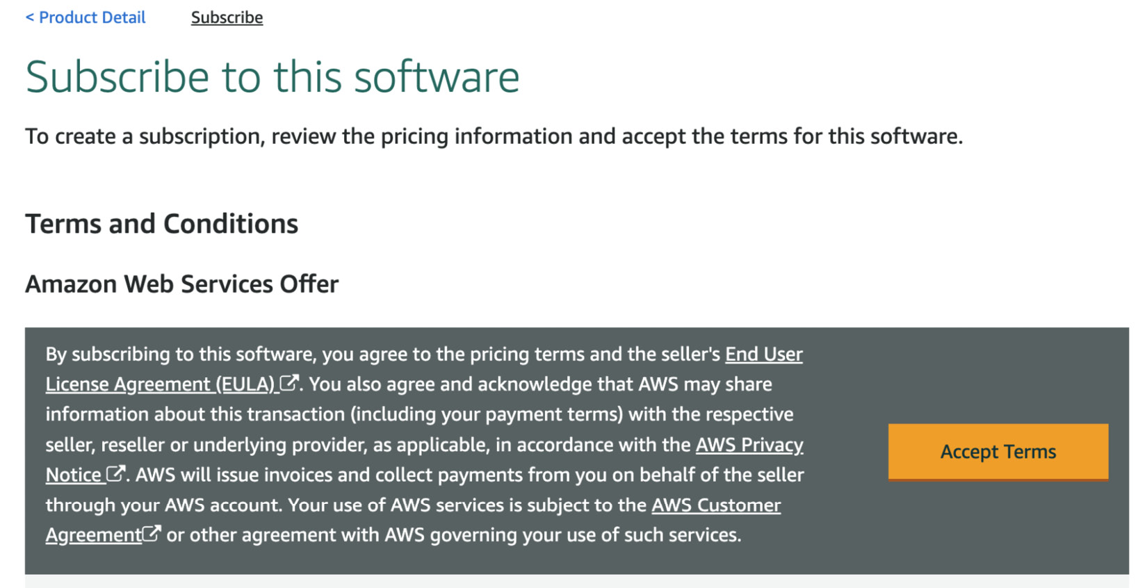
Figure 13.2 – Accept the terms

3. After some time, when your request has been processed, the Continue to Configuration button will be enabled. Click on it:
   

Figure 13.3 – The Continue to Configuration button

4. Select Glue 3.0 as the Fulfillment option setting, select 0.9.0 (Feb 16, 2022) as the Software version setting, and click on the Continue to Launch button that is present in the upper-right corner of the screen:

Figure 13.4 – Fill in the required options

5. Click on the Usage instructions link:

Figure 13.5 – Launch the software

6. Click on the Activate the Glue connector from AWS Glue Studio link:

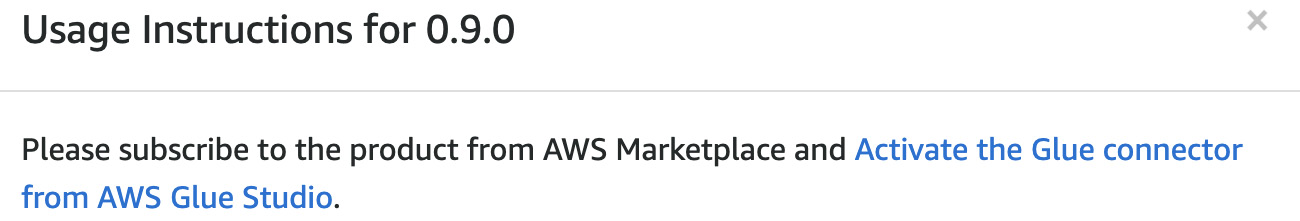
Figure 13.6 – Activating the Glue connector

7. Give a name to the connection, and then click on the Create connection and activate connector button. Make a note of the name of the connection. This will be one of the inputs to the CloudFormation template:

Figure 13.7 – Create a connection

Now we will follow the same process for creating Delta Lake and Amazon OpenSearch connections.

Creating a Delta Lake connection

Search for Delta Lake Connector for AWS Glue in the Marketplace. We will use 1.0.0-2 (Feb 14, 2022) as the Software version setting and Glue 3.0 as the Fulfilment option setting. Make a note of the name you give to the connection. This name will be an input to the CloudFormation template.

Creating an OpenSearch connection

Search for Elasticsearch Connector for AWS Glue in the Marketplace. Use the one owned by Amazon Web Services. We will use 7.13.4-2 (Feb 14, 2022) as the Software version setting and Glue 3.0 as the Fulfilment option setting. Make a note of the name you give to the connection. This name will be an input to the CloudFormation template:

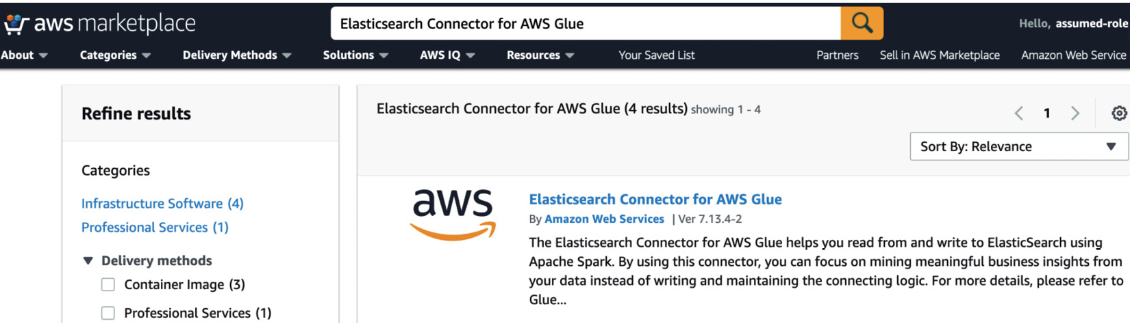
Figure 13.8 – Elasticsearch Connector for AWS Glue

Now we will be creating a CloudFormation stack. The stack will create all the network elements such as VPCs, subnets, and security groups along with Glue jobs and other resources such as a Redshift cluster, an OpenSearch cluster, and an MSK cluster. These resources will help you to successfully execute the Glue jobs associated with various sections of this chapter.

Creating the CloudFormation stack

First, let’s go through the prerequisites for this section.

Prerequisites for creating the CloudFormation stack

Make sure that the Amazon OpenSearch, Delta Lake, and Apache Hudi connections have been created. Also, make sure that you have a KeyPair. This KeyPair will be used to connect to one of the EC2 instances created by the CloudFormation template.

The CloudFormation template will create IAM roles and policies, too. These roles and policies are required for the jobs to function. Please review the definition of these roles, policies, networks, and security groups, and ensure that they align with the standards of your organization. In the following sections, first, we will create the stack and then create the dataset.

Creating the stack

The CloudFormation stack creates 61 resources. These resources can be found in the Resources tab of the CloudFormation stack.

Import the template in CloudFormation and enter the name of the stack, the name of the Apache Hudi Marketplace connection, the name of the Delta Lake Marketplace connection, the name of the Amazon OpenSearch connection, the username and password for both the Redshift master user and the Amazon OpenSearch master user, the IP of your laptop, and the KeyPair that will be used to connect to the EC2 created by the CloudFormation (CFn). Keep the default settings for the rest of the parameters.

Please note that the password for Amazon OpenSearch master user must have at least 8 characters: one uppercase character, one lowercase character, one number, and one of the #$! special characters. The password for the Redshift master user must have at least 8 characters: one uppercase character, one lowercase character, and one number. Special characters are not allowed.

After the CloudFormation stack has been created, follow the next section to create a dataset.

Creating a dataset

Before we start looking at various techniques for data analysis, let’s start by creating a basic dataset to work with.

Navigate to the AWS Glue Studio console (https://console.aws.amazon.com/gluestudio/home), check the checkbox next to the 01 - Seed data job for Data Analysis Chapter job, and click on the Run Job button:

Figure 13.9 – The AWS Glue Studio console

The CloudFormation template shipped with this chapter will have created this job and the associated resources, such as the S3 bucket, the IAM roles and policies, and the AWS Glue Catalog database, that are required to run the job.

Now you can go to the AWS Glue Studio monitoring page (https://console.aws.amazon.com/gluestudio/home?#/monitoring) and check the status of the job. Note that you might see a lag for a few seconds for the job execution to be reflected on the AWS Glue Studio monitoring page (https://console.aws.amazon.com/gluestudio/home?#/monitoring):

Figure 13.10 – Checking the status of the jobs

The successful completion of this job will create an employees table in chapter-data-analysis-glue-database.

Now that we have some data, let’s understand the past and current patterns of data analysis.

The benefit of ad hoc analysis and how a data lake enables it

Before the start of the data lake pattern, organizations used to offload their data into a data warehouse for analysis. This involved creating an Extraction, Transformation, and Load (ETL) pipe. Creating ETL pipes, moving the data into a warehouse, and creating reports take a substantial amount of time and resource investment. By the time all of this has finished, the requirements will have changed because of the change in the business over a period of time. Sometimes, business users discovered that they didn’t get what they ordered and that there was a gap in requirement and implementation.

For example, a business user could request sales data, resulting in the IT team moving the sales data into the warehouse. However, the sales data in the warehouse might not be of the grain that the business user needs or does not include the sales data from all the sources of sales information. All of this involves a massive amount of rework.

With the advent of data lakes, organizations moved from code to configuration. Unlike a data warehouse, which requires the creation or modification of an ETL job, bringing a new source into the data lake usually involves adding a configuration to existing pipes. This is possible because the first layer of a data lake is generally the raw or the bronze layer and, usually, involves an extract and load job. Data is brought into this layer in a business-agnostic fashion. Since there is no transformation involved, the same jobs can be reused to bring in newer sources.

This hugely reduces the time required to make the data available, as bringing it from a new source to the data lake no longer requires any development effort and is, now, purely an operations ticket. However, this data in the raw/bronze layer is generally in the format of the source and is not standardized. This brings about the need for a semi-processed layer. This is generally called the silver layer.

Generally, the transformation between the bronze layer and the silver layer is also business agnostic. This is because the silver layer is considered the single source of truth for all downstream systems. We don’t know what requirements we might have in the future. Hence, transforming the data in any way creates a possibility of not being able to transform it differently if we get such a requirement in the future.

However, the transformation from bronze to silver includes common sense operations such as partitioning, compression, the addition of audit columns, and creating derived fields. All of these operations are coded such that the jobs remain reusable for any new sources that we might have to bring in. The transformed data can be easily pulled by all the downstream systems that need it. Additionally, the transformations are designed to provide traceability to the ops team if they have to troubleshoot some data inconsistency in the downstream systems.

By now, we understand that the data is made available in the silver bucket using reusable code, but how do we access this data? That is where the central metadata catalog comes in. The AWS Glue Data Catalog can be the central repository of metadata, and the metadata can either be updated from within the Glue jobs or using AWS Glue crawlers. Other services, such as Amazon Athena and Amazon EMR, can also update the AWS Glue Data Catalog. The AWS Glue Data Catalog (https://docs.aws.amazon.com/glue/latest/dg/components-overview.html#data-catalog-intro) is also accessible from other AWS services such as Amazon EMR, Amazon RDS, Amazon Redshift Spectrum, Amazon Athena, and any application that is compatible with the Apache Hive metastore. Additionally, you can configure the AWS Glue Data Catalog of a different AWS account (https://docs.aws.amazon.com/athena/latest/ug/data-sources-glue-cross-account.html).

With this feature, business analysts do not have to wait for the creation of the ETL pipelines for the data to be available in the warehouse but can directly query the silver bucket using the AWS Glue Data Catalog. This enables them to do an analysis of the data and understand exactly which transformation has to be formalized and coded into the ETL pipelines and brought to the warehouse. This saves a lot of IT effort.

Now, that we understand the tangible benefit of ad hoc analysis and how a data lake enables it, let’s look at the two primary means of computing in AWS that are used for ad hoc analysis. They are Amazon Athena and Amazon Redshift Spectrum.

Amazon Athena

Amazon Athena is a serverless interactive query service, based on the Presto platform, that can leverage the AWS Glue Data Catalog for getting the table metadata. Because Amazon Athena is serverless, there is no infrastructure to set up or manage.

While we will primarily use Amazon Athena for querying purposes, it can do a lot more than just that. We will spend the next few paragraphs learning about some of the most important features of Amazon Athena and what makes it so powerful. We discuss these features because Amazon Athena is one of the most important and widely used tools for data exploration and analysis in the AWS world. Having a good understanding of Amazon Athena is going to be important to be effective in data exploration on AWS.

Amazon Athena uses an asynchronous query arrangement. When a user submits a SQL query, Amazon Athena uses a hot cluster to execute the query and then writes the processed result into a temporary S3 location. Then, these results are read and returned to the client. You can use the AWS portal to use Amazon Athena, or you can also use the Athena JDBC driver (https://docs.aws.amazon.com/athena/latest/ug/connect-with-jdbc.html) in any application, such as SQL Workbench (https://www.sql-workbench.eu/downloads.html), that supports a JDBC connection. Additionally, you can use the identities stored in Okta for configuring federated access to Athena using JDBC and Lake Formation (https://docs.aws.amazon.com/athena/latest/ug/security-athena-lake-formation-jdbc-okta-tutorial.html). You can also use Microsoft’s Azure Active Directory (AD) or Ping Identity’s PingFederate for authentication. Additionally, you can choose to use the Amazon Athena ODBC drivers (https://docs.aws.amazon.com/athena/latest/ug/connect-with-odbc.html).

Recently, Amazon Athena upgraded to version 2 of the Athena engine, which is based on Presto 0.217. This brings new features and performance enhancements to the JOIN, ORDER BY, and AGGREGATE operations.

The integration with the AWS Glue Data Catalog allows the creation of a unified metadata repository across multiple AWS services. While the AWS Glue Data Catalog is generally used for the unified metadata store, you can also connect Athena to an external Hive metastore (https://docs.aws.amazon.com/athena/latest/ug/connect-to-data-source-hive.html).

In Amazon Athena, most results are delivered within seconds, and you are charged based on the amount of data scanned by the query (https://aws.amazon.com/athena/pricing/). Because you are charged for the amount of data scanned, you can greatly reduce your bills by following the best practices related to compression and partitioning that were introduced in Chapter 5, Data Layout. Also, you can use Amazon Athena workgroups to track costs, and control and set limits on each workgroup to control costs. You can also add tags to these workgroups and then use Tag-Based IAM access policies (https://docs.aws.amazon.com/athena/latest/ug/tags-access-control.html) to control permissions.

Amazon Athena query metrics can be published to CloudWatch. Then, these metrics can be used to create alarms that can trigger actions based on the alarms. Also, you can also use the Explain Analyze (https://docs.aws.amazon.com/athena/latest/ug/athena-explain-statement.html) statement in Amazon Athena to get the computational cost of each operation in a SQL query.

Additionally, Amazon Athena can use the fine-grained access control rules set up in your AWS Lake Formation. AWS Lake Formation allows administrators to configure column-, row-, and even cell-level permissions (https://docs.aws.amazon.com/lake-formation/latest/dg/data-filtering.html).

Amazon Athena also supports Atomicity, Consistency, Isolation, and Durability (ACID) transactions to allow for DML operations such as inserts, updates, and deletes along with the ability to time travel. This ACID transaction feature (https://docs.aws.amazon.com/athena/latest/ug/acid-transactions.html) is based on the open source Apache Iceberg (https://iceberg.apache.org/). Additionally, Amazon Athena supports read operations on AWS Lake Formation governed tables and Apache Hudi tables (https://docs.aws.amazon.com/athena/latest/ug/querying-hudi.html).

Apart from querying the data in S3, you can also query the data in other data stores such as Amazon CloudWatch Logs, Amazon DynamoDB, Amazon DocumentDB, and Amazon RDS, and JDBC-compliant relational data sources, such as MySQL and PostgreSQL, under the Apache 2.0 license using Amazon Athena Federated Query feature (https://docs.aws.amazon.com/athena/latest/ug/connect-to-a-data-source.html). Prebuilt Athena data source connectors exist for these sources. You can also deploy your own connector to connect to a data source (https://docs.aws.amazon.com/athena/latest/ug/connect-to-a-data-source-lambda.html).

Amazon Athena is also used in combination with AWS Step Functions (https://aws.amazon.com/step-functions/) to create a data processing pipeline that is orchestrated in AWS Step Functions and processed using Amazon Athena. These data processing pipelines can use User-Defined Functions (UDFs) (https://docs.aws.amazon.com/athena/latest/ug/querying-udf.html) in Amazon Athena for reusable and standardized processing that has to be used multiple times within the same pipeline or across multiple pipelines. Additionally, the same USING EXTERNAL FUNCTION syntax that was used with UDFs can be used to run the ML inference using Amazon SageMaker (https://aws.amazon.com/sagemaker/). Now, let’s look at some of the Amazon Athena features that can help us be more efficient in querying data.

You can create views in Athena to simplify the querying process for less SQL-savvy resources and to ensure consistent results for common queries.

Often, data exploration requires parsing nested structures and arrays. Amazon Athena supports both of these and can also parse a JSON object. This flexibility to parse complex structures helps Amazon Athena enable data exploration on less-than-perfect data. Amazon Athena also supports queries on geospatial data. The input data should be in WKT (Well-known text) format or JSON-encoded geospatial data format. Amazon Athena can also be configured to query AWS CloudTrail logs, Amazon CloudFront logs, Classic Load Balancer logs, Application Load Balancer logs, Amazon VPC flow logs, and Network Load Balancer logs.

Additionally, you can parameterize the queries that are used more often. This is done using the PREPARE and EXECUTE statements (https://docs.aws.amazon.com/athena/latest/ug/querying-with-prepared-statements.html). You also have the option to save the queries per workgroup.

Querying in Athena

In the previous section, we learned about the various features of Athena that can help to simplify data exploration in AWS. In this section, we will look at a simple example for querying the data.

Run the following query in your Athena console. You should be able to see the data inserted in the 01 - Seed data job for Data Analysis Chapter job in the Creating a dataset section:

SELECT * FROM "AwsDataCatalog"." chapter-data-analysis-glue-database"."employees" order by emp_no;

You will see the following output:

Figure 13.11 – Query output in the Athena console

So far, we have created sample data using Glue jobs, we have learned about the various features for data exploration in Athena, and we have also queried our sample data through Athena.

Next, we will look at another tool for exploring data in Amazon S3.

Amazon Redshift Spectrum

Redshift Spectrum is a feature within the Redshift toolset. It is a mechanism used to query S3 data by employing massive parallelism to query the data on a big data scale. The feature also enables Redshift to offload a part of the query compute such as aggregation and filtering to the spectrum layer. Just like Athena, Amazon Redshift Spectrum can query data from the AWS Glue Data Catalog or an external Hive metastore. So, tables created in the AWS Glue Data Catalog can be accessed within Redshift through Redshift Spectrum using an external schema. Later in this section, we will check a related example.

Users can also partition the data, and the intelligent spectrum layer can prune those partitions when users query for the specific data within the partitions. Because the data lives externally, the same data can be accessed in multiple Redshift clusters through the spectrum layer. Other big data technologies such as Hudi can be used to create a transactional data lake. Redshift supports Copy-on-Write (CoW) Hudi tables (https://hudi.apache.org/docs/concepts.html#copy-on-write-table). Check out the documentation (https://docs.aws.amazon.com/redshift/latest/dg/c-spectrum-external-tables.html#c-spectrum-column-mapping-hudi) for supported Hudi versions. We will discuss Hudi tables in more detail in the following sections. Updates to the CoW Hudi tables are available in Redshift through the Spectrum layer.

Additionally, you can query Delta Lake (https://delta.io/) tables through Redshift Spectrum. The data from Redshift Spectrum can be joined with the data maintained within Redshift. You can also use data handling options (https://docs.aws.amazon.com/redshift/latest/dg/t_setting-data-handling-options.html) to define Spectrum’s behavior when it finds unexpected values in the columns of external tables. Spectrum supports the row and column level rules that have been set up for your data lake security for governed tables. Additionally, data in S3 accessed via Spectrum can be used to hydrate the materialized views in Redshift (https://docs.aws.amazon.com/redshift/latest/dg/materialized-view-overview.html).

One of the major improvements in Spectrum, which was introduced a few years ago, was the support for bloom filters. A bloom filter is a probabilistic, memory-efficient data structure that accelerates join queries. Redshift decides on its own whether to use the bloom filter for a query at runtime. Spectrum supports modern BI tools by enabling you to query for complex and nested data types (https://docs.aws.amazon.com/redshift/latest/dg/tutorial-query-nested-data.html) such as structs, arrays, or maps in S3 data.

Now that we understand Redshift Spectrum, let’s create an external schema in Redshift to query the table that we created using the 01 - Seed data job for Data Analysis Chapter job in the Creating a dataset section.

The CloudFormation template shipped with this chapter creates a role called HandsonSeriesWithAWSGlueRSRole and a Redshift cluster to enable us to use Amazon Redshift Spectrum to query the data from S3. Please navigate to the IAM console (https://console.aws.amazon.com/iamv2/home#/roles/details/HandsonSeriesWithAWSGlueRSRole) and check out the definition of this role to ensure that it is compliant with your organization. This role will be used by Amazon Redshift to access the AWS Glue Data Catalog:

1. Go to the Redshift SQL workbench console (https://console.aws.amazon.com/sqlworkbench/home?#/client).
2. Click on the Redshift cluster created by the CloudFormation template. You can get this from the RedshiftClusterId key of the Outputs tab of the CloudFormation stack:

Figure 13.12 – The Redshift cluster in Redshift query editor v2

3. Select the Database user name and password option and enter the username and password entered during the creation of the CloudFormation stack. You can keep the default value of dev for the Database field. Click on the Create connection button:

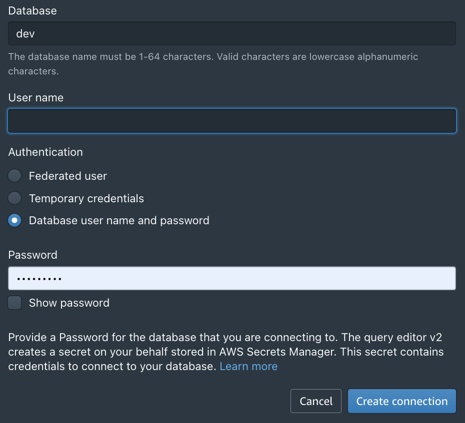
Figure 13.13 – The Database username and password options

4. Make sure that the dev database has been selected at the top:

Figure 13.14 – Selecting the dev database

5. Enter the following command, and click on the Run button:

   create external schema chapter_data_analysis_schema from data catalog database 'chapter-data-analysis-glue-database' region '<region>'  iam_role 'arn:aws:iam::<aws_account_id>:role/HandsonSeriesWithAWSGlueRSRole';

Replace region and aws_account_id in the preceding command.

Here, database is the AWS Glue Data Catalog database. This database was created through the CloudFormation stack.

6. Now, expand the dev database. You should notice the chapter_data_analysis_schema schema underneath it. Now you should be able to see the employees table created in the Creating a dataset section:

Figure 13.15 – Expanding the dev database option

7. Run the following SELECT query to see the data loaded into the Glue Data Catalog table:

   SELECT * FROM "dev"."chapter_data_analysis_schema"."employees" order by emp_no;

The output is as follows:

Figure 13.16 – Data in the Glue Data Catalog table

Alright, so we saw how the data written in S3 can be accessed by both Redshift and Athena for analysis. But what if the data had to be updated? One mechanism is to overwrite, that is, truncate and then load the table. In some cases, this approach can be expensive. We can probably come up with a more cost-optimized approach where we, first, partition the table and then only overwrite a partition. However, this approach comes with its own drawbacks.

For this approach to work, the newer updates will have to be limited to only a few of the partitions because if the newer updates are across partitions, then all of the partitions will have to be overwritten. As you might have noticed, creating a logic to upsert data in a data lake can become quite complex very quickly. An alternative is to use open source solutions such as Hudi and Delta Lake to make the data lake more transactional. Solutions such as Hudi bring additional benefits, such as the ability to create Merge on Read (MoR) or CoW (tables along with the ability to only query the incremental data and time travel.

In order to simplify the process of using these open source technologies, the AWS Glue team came up with AWS Glue custom connectors (https://aws.amazon.com/about-aws/whats-new/2020/12/aws-glue-launches-aws-glue-custom-connectors/).

In this chapter, we will use quite a few Marketplace Glue connectors. Previously, you created Apache Hudi, Delta Lake, and OpenSearch connections in the Creating Marketplace connections section. Now we will use Apache Hudi and Delta Lake connections for upserting data in the S3 data lake.

Creating and updating Hudi tables using Glue

Apache Hudi is an open source data management tool that was initially developed by Uber. Its superpower is enabling incremental data processing in a data lake. The Apache Hudi format is supported by a wide range of tools on AWS such as AWS Glue, Amazon Redshift, Amazon Athena, and Amazon EMR.

The CloudFormation template, for this chapter, creates two Hudi batch jobs. They are 02 - Hudi Init load for Data Analysis Chapter and 03 - Hudi Incremental load for Data Analysis Chapter. Both of these jobs use the Hudi connection created in the Creating the Marketplace connections section. Additionally, these jobs accept the target bucket as an input parameter. This input parameter is prepopulated by the CloudFormation template. Navigate to the job details page of the 02 - Hudi Init load for Data Analysis Chapter job (https://console.aws.amazon.com/gluestudio/home?#/editor/job/02%20-%20Hudi%20Init%20load%20for%20Data%20Analysis%20Chapter/details) to check out the configurations for the job.

Now we will execute the Glue Hudi jobs to create Hudi tables in the Glue Data Catalog:

1. Navigate to the AWS Glue Studio console (https://console.aws.amazon.com/gluestudio/home?#/jobs), check the checkbox next to 02 - Hudi Init load for Data Analysis Chapter, and click on the Run Job button.
2. Now you can go to the AWS Glue Studio monitoring page (https://console.aws.amazon.com/gluestudio/home?#/monitoring) and check the status of the job. You might see a lag of a few seconds for the execution to show up on the monitoring page:

Figure 13.17 – Viewing the job status

3. After the job finishes, this job will create a Hudi table, and you will be able to query it in Athena using the following query:

   SELECT emp_no, name, department, city, salary FROM "AwsDataCatalog"."chapter-data-analysis-glue-database"."employees_cow" order by emp_no;

The results are as follows:

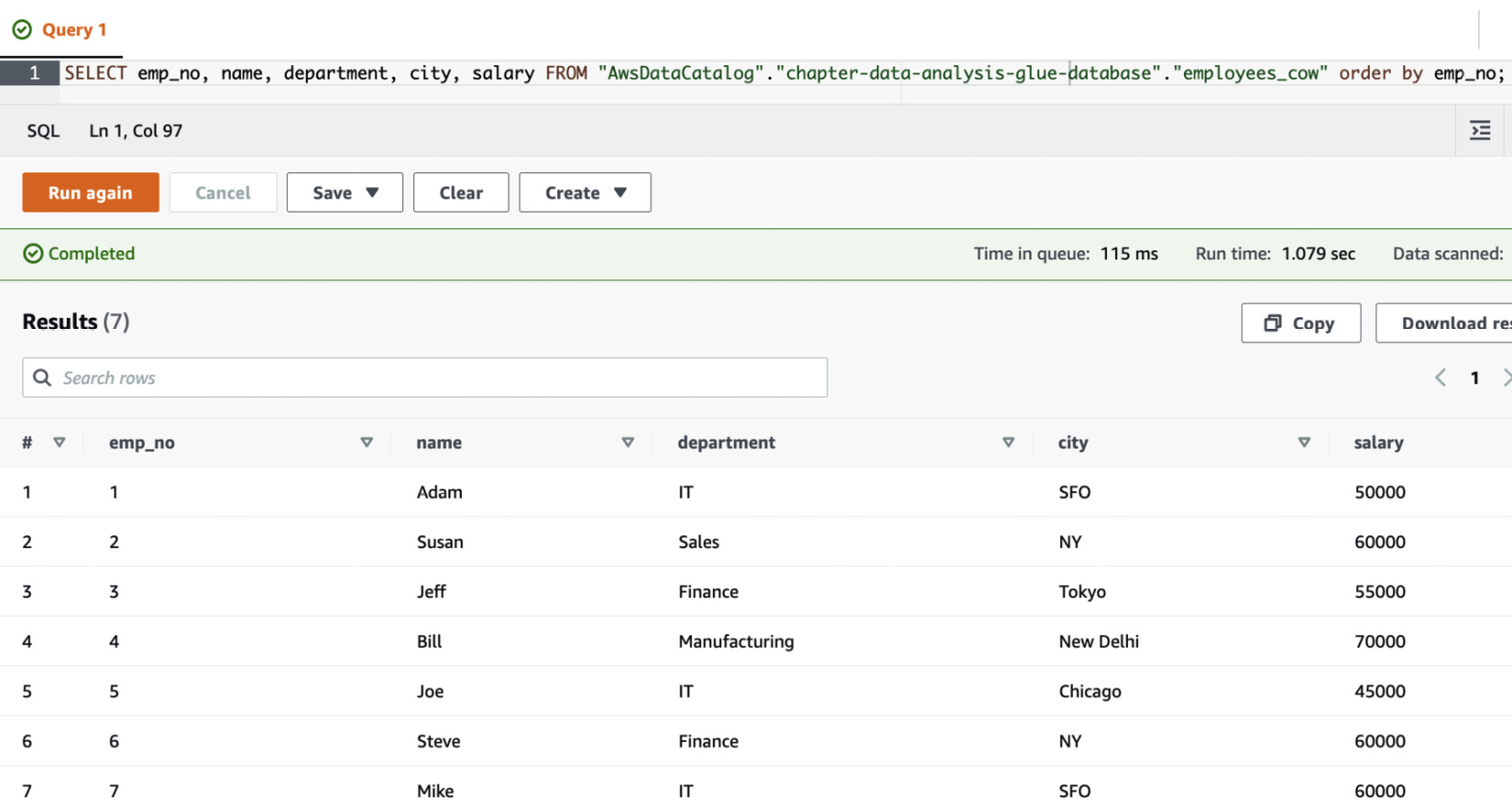
Figure 13.18 – The query results for the Hudi table

4. Now, let’s say that Jeff got a raise along with a transfer to Cincinnati. Additionally, let’s say that Jeff’s new salary is 75,000. Run the 03 - Hudi Incremental load for Data Analysis Chapter job just as you ran the previous one. This job will help to update the information in the employees_cow table. Note that the value of salary=75000 and city=Cincinnati for emp_no=3 is hardcoded in this job.
5. Go to the go the AWS Glue Studio monitoring page (https://console.aws.amazon.com/gluestudio/home?#/monitoring) and check the status of the job. You might see a lag of a few seconds for the execution to show up on the monitoring page:

Figure 13.19 – Monitoring the status of the 03 - Hudi Incremental load for Data Analysis Chapter job

6. After the successful completion of the job, run the query on the employees_cow table in Amazon Athena again. You will notice that the record has been updated:

   SELECT emp_no, name, department, city, salary FROM "AwsDataCatalog"."chapter-data-analysis-glue-database"."employees_cow" order by emp_no;

The results are as follows:

Figure 13.20 – The updated table

We just saw the use of Apache Hudi for upserting the data in a lake and querying the upserted data in Athena. Now we will try to upsert the data using the Delta Lake connection created in the Creating Marketplace connections section.

Creating and updating Delta Lake tables using Glue

Delta Lake is also an open source framework that was initially developed by Databricks. Similar to Hudi, Delta Lake is also supported by Spark, Presto, and Hive among many others.

We will now execute the 04 - DeltaLake Init load for Data Analysis Chapter job to create a Delta Lake table. The 04 - DeltaLake Init load for Data Analysis Chapter job was created by the CloudFormation template executed earlier:

1. Run the Glue job: 04 - DeltaLake Init load for Data Analysis Chapter. Notice in the job script that we are using Spark SQL to create a table definition in the Glue Catalog for the Delta Table. Here is the Spark SQL statement from the code of the 04 - DeltaLake Init load for Data Analysis Chapter job:

   spark.sql("CREATE TABLE `chapter-data-analysis-glue-database`.employees_deltalake (emp_no int, name string, department string, city string, salary int) ROW FORMAT SERDE 'org.apache.hadoop.hive.ql.io.parquet.serde.ParquetHiveSerDe' STORED AS INPUTFORMAT 'org.apache.hadoop.hive.ql.io.SymlinkTextInputFormat' OUTPUTFORMAT 'org.apache.hadoop.hive.ql.io.HiveIgnoreKeyTextOutputFormat' LOCATION '"+tableLocation+"_symlink_format_manifest/'")

Also, notice that we have put /tmp/delta-core_2.12-1.0.0.jar in the Python lib path argument. This can be seen in the following screenshot:

Figure 13.21 – Running the 04 - DeltaLake Init load for Data Analysis Chapter job

Additionally, we generate symlink_format_manifest from within the Glue job. This helps us to read the table from Athena or Presto.

2. Go to the AWS Glue Studio monitoring page (https://console.aws.amazon.com/gluestudio/home?#/monitoring) and check the status of the job. Once the job is complete, go to Athena, and execute the following statement:

   SELECT * FROM "AwsDataCatalog"."chapter-data-analysis-glue-database"."employees_deltalake" order by emp_no;

You will notice that the data has been inserted into the Glue Catalog table and can be queried through Athena, as shown in the following screenshot:

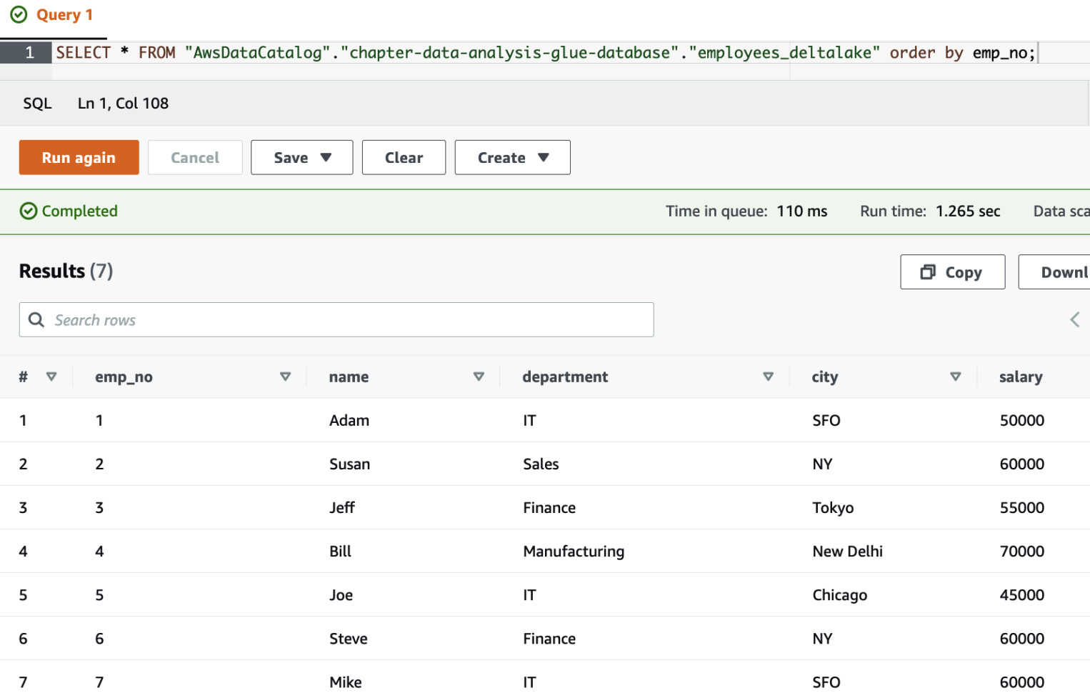
Figure 13.22 – The result of the executed statement

3. Now, let’s say that we want to update city to Cincinnati and salary to 70000 for emp_no = 3. Run the 05 - DeltaLake Incremental load for Data Analysis Chapter job and let it finish. The value of salary=75000 and city=Cincinnati for emp_no=3 is hardcoded into this job.
4. Run the following query in Athena and notice that the data for emp_no = 3 has changed:

   SELECT * FROM "AwsDataCatalog"."chapter-data-analysis-glue-database"."employees_deltalake" order by emp_no;

The results are as follows:

Figure 13.23 – The updated data for emp_no = 3

In this section, we saw how we can create and update tables and data in the Glue Data Catalog using Delta Lake. Now we will look at how we can insert data into governed tables.

Inserting data into Lake Formation governed tables

Governed tables are packed with a lot of features such as ACID transactions, automatic data compaction for faster query response times, and time travel queries. Now we will go through the process of creating Lake Formation governed tables using Glue jobs:

1. Go to the Outputs tab of the CloudFormation stack and grab the S3 path for the LakeFormationLocationForRegistry key.
2. Go to AWS Lake Formation (https://console.aws.amazon.com/lakeformation/home) and register the S3 location, from step 1, with Lake Formation, as shown in the following screenshot:

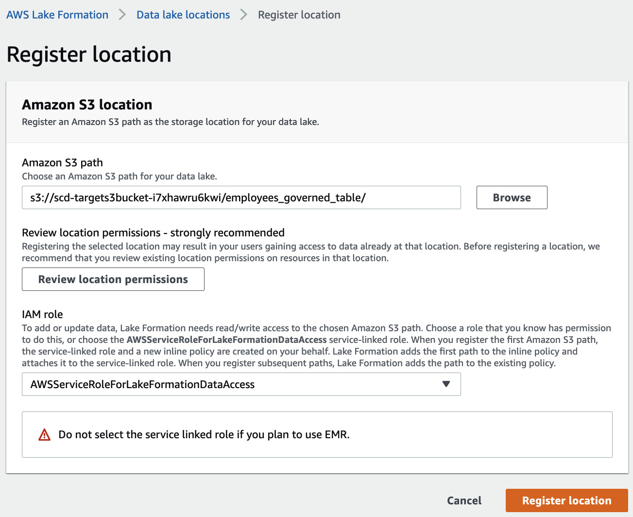
Figure 13.24 – Registering the location

The format of this path is s3://<target_s3_bucket>/employees_governed_table/. Make sure that you register it in the same region where you created the Cloud Formation stack.

Note that you should use the AWSServiceRoleForLakeFormationDataAccess role. This role has been granted access to the KMS key so that we can query the governed table successfully.

3. Go to Data locations tab in Lake Formation and grant privileges from s3://<target_s3_bucket>/employees_governed_table/ to HandsonSeriesWithAWSGlueJobRole. You will have to paste the s3://<target_s3_bucket>/employees_governed_table/ path inside the Storage locations textbox and select HandsonSeriesWithAWSGlueJobRole from the IAM users and roles drop-down list:

Figure 13.25 – The Data locations tab

4. Run the 06 - Governed Table Create Table for Data Analysis Chapter job from Glue Studio, just as you ran the previous jobs. This job will create employees_governed_table in chapter-data-analysis-glue-database. After the job has been successfully completed, you should be able to see the table in Athena.
5. Now we will load this table with data. Execute the 07 - Governed Table Init Load for Data Analysis Chapter job. This code starts a transaction, loads the data, and then commits it.
6. After the job finishes, you will now be able to query the data in Athena. Run the following command:

   SELECT * FROM "AwsDataCatalog"."chapter-data-analysis-glue-database"."employees_governed_table" order by emp_no;

The following screenshot shows the data in the employees_governed_table table:

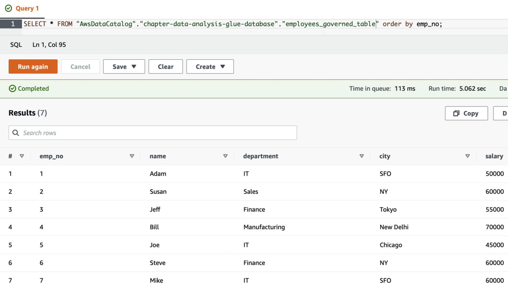
Figure 13.26 – Data in the employees_governed_table table

In this section, we saw how governed tables can be used to ingest data in a data lake. The Glue job used to ingest the data ran as a batch. In fact, in this chapter, all of the jobs that have been executed so far have been batch jobs. These jobs include the jobs related to both Hudi and Delta Lake. Next, we will look at how to stream ingestion jobs.

Consuming streaming data using Glue

Now that we understand how Glue works in batch mode, let’s understand the process of updating the data coming through a stream.

The CloudFormation stack creates a Managed Streaming for Apache Kafka (MSK) cluster for this purpose. You will have to create a Glue connection for this MSK cluster. It is important that you name this connection as chapter-data-analysis-msk-connection. This connection is used in the jobs that follow. These jobs get the Kafka broker details from the connection.

Creating chapter-data-analysis-msk-connection

We will execute Glue jobs to load data into an MSK topic and also consume data from the topic. Both of these jobs require broker information and other details about the MSK cluster. Now we will create an MSK connection in Glue. Please ensure that you put the name of the connection as chapter-data-analysis-msk-connection. This is because the Glue jobs have been preconfigured to use this name as the connection name:

1. Navigate to the Connections page in the AWS Glue console (https://console.aws.amazon.com/glue/home?#catalog:tab=connections), and then go to the Connections section.
2. Click on the Add connection button.
3. Set Connection type as Kafka and put Connection name as chapter-data-analysis-msk-connection. Select the MSK cluster created using CloudFormation in the Select MSK cluster drop-down list and ensure that the Require SSL connection flag has been checked. Click on Next:

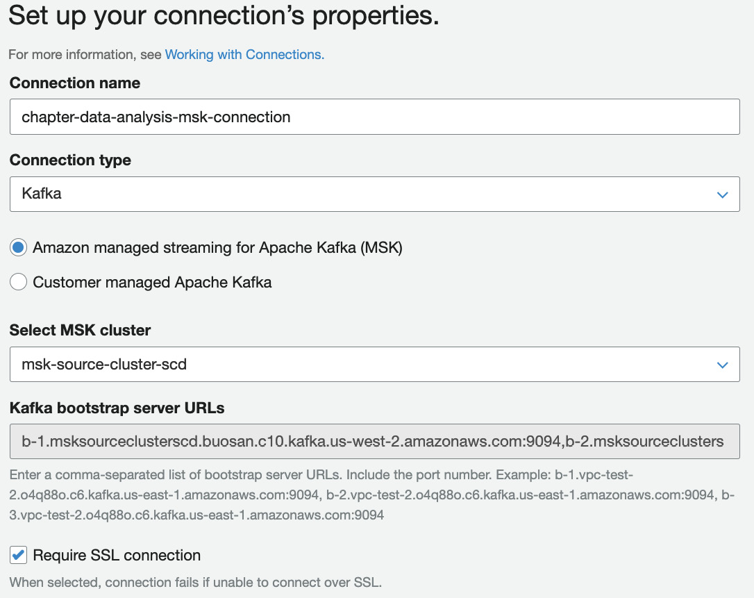
Figure 13.27 – Setting up the properties

4. Select the VPC ID, one of the private subnet IDs, and a security group, and click on Next. You should be able to get all of these values from the Outputs tab of the CloudFormation stack. Click on Finish:

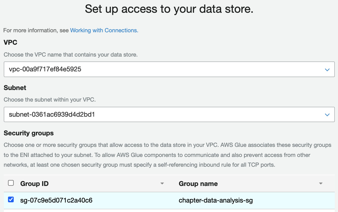
Figure 13.28 – Setting up access

Now that we have created an MSK connection in Glue, we will load data into a topic in the MSK cluster. Later, we will consume data from the topic through Glue streaming jobs.

Loading and consuming data from MSK using Glue

Run the Python shell’s 08 - Kafka Producer for Data Analysis Chapter job. This job will use chapter-data-analysis-msk-connection, as created in the preceding section, and load data into the MSK cluster.

This job uses the AWS wrangler whl file and the kafka-python whl file to read the data from the S3 path and load it into Kafka. Both of these whl files have been copied in the S3 bucket of your account through the CloudFormation template and have been configured in the Glue Python shell job. This job creates a chapter-data-analysis topic and then loads data into it.

After the job has successfully finished, you will have the data in the MSK cluster. Now we should execute the Glue streaming jobs to consume the data from the topic.

Glue streaming job as a consumer of a Kafka topic

First, we will check out the traditional micro-batch pattern that is commonly employed to consume streaming data using Glue.

Start the 09 - Kafka Consumer for Data Analysis Chapter job. This is a Spark streaming job that consumes data from the chapter-data-analysis topic. It micro-batches the processing using the forEachBatch (https://docs.aws.amazon.com/glue/latest/dg/aws-glue-api-crawler-pyspark-extensions-glue-context.html#aws-glue-api-crawler-pyspark-extensions-glue-context-forEachBatch) method of GlueContext.

The forEachBatch method micro-batches the streaming dynamic frame. In the 09 - Kafka Consumer for Data Analysis Chapter job, the micro-batch is 10 seconds. Each micro-batch is processed in the processBatch method. In the 09 - Kafka Consumer for Data Analysis Chapter job, we write the micro-batch into a Hudi table just as we had written one in the batch operation.

Notice that the processing of these micro-batches was no different from the processing of the Hudi batch jobs shared earlier. Essentially, this means that the process can be applied to consume a stream in other formats such as Delta Lake using the batch code for the Delta Lake shared earlier.

After a couple of minutes of execution, you should see the employees_cow_streaming table under chapter-data-analysis-glue-database. You should be able to query it in Athena using the following query:

SELECT emp_no,name,department,city,salary FROM "AwsDataCatalog"."chapter_data_analysis"."employees_cow_streaming" order by emp_no;

The results are as follows:

Figure 13.29 – The results of the query

In this section, we used a streaming Glue job to consume data from a Kafka topic. In the next section, we will use the Hudi DeltaStreamer (https://hudi.apache.org/docs/hoodie_deltastreamer/) utility to consume data from the same Kafka topic.

Hudi DeltaStreamer streaming job as a consumer of a Kafka topic

Now that we have seen the traditional micro-batch method used to consume streaming sources in Hudi tables using Glue, let’s look at the mechanism of using Hudi DeltaStreamer to consume streaming data.

Run the 10 - DeltaStreamer Kafka Consumer for Data Analysis Chapter job. Just as in the previous job, this also uses the Hudi connection. However, notice that the dependent JARs path has been set to /tmp/*. This is required to ensure that the right classes are available on the classpath. While some of the configurations are similar to the configurations of the Hudi jobs that we created up till now, the DeltaSteamer job requires the schema files for the source and target. Since our use case is about replicating data, our source and target schema has the same file. The structure of this avro schema file is as follows:

{

  "type":"record",

  "name":"employees",

  "fields":[{

     "name": "emp_no",

     "type": "int"

  }, {

     "name": "name",

     "type": "string"

  }, {

     "name": "department",

     "type": "string"

  },{

     "name": "city",

     "type": "string"

  },{

     "name": "salary",

     "type": "int"

  },{

     "name": "record_creation_time",

     "type": "float"

  }

]}

This file is written into your S3 bucket through CloudFormation, and the 10 - DeltaStreamer Kafka Consumer for Data Analysis Chapter job is configured to use this avro schema file.

Once the job has been executing for 2–3 minutes, you should be able to see and query the employees_deltastreamer table in chapter-data-analysis-glue-database, in Athena, using the following query:

SELECT emp_no,name,department,city,salary FROM "AwsDataCatalog"."chapter-data-analysis-glue-database"."employees_deltastreamer" order by emp_no;

The result is as follows:

Figure 13.30 – The 10 - DeltaStreamer Kafka Consumer for Data Analysis Chapter job results

Now we have our traditional Glue streaming and DeltaStreamer jobs running. This means that if we add new data to our MSK topic, the data will be consumed by both of our jobs. Now we will load CDC data into our topic. Our streaming jobs should consume and process the data. Our query through Athena should be able to show the updated data in the processed tables since our streaming jobs are using Hudi.

Creating and consuming CDC data through streaming jobs on Glue

Now, we will load CDC data into the MSK topic.

Run the 11 - Incremental Data Kafka Producer for Data Analysis Chapter job. This job adds the following CDC data to the chapter-data-analysis topic:

{"emp_no": 3,"name": "Jeff","department": "Finance","city": "Cincinnati","salary": 70000,"record_creation_time":now}

This job uses the same whl files as the 08 - Kafka Producer for Data Analysis Chapter job.

As soon as the job finishes, you should be able to see the update in both the employees_deltastreamer and employees_cow_streaming tables. The following screenshot shows the result in the employees_deltastreamer table:

Figure 13.31 – The results of the employees_deltastreamer table

The following screenshot shows the result in the employees_cow_streaming table:

Figure 13.32 – The results of the employees_cow_streaming table

Since our Glue streaming jobs are configured to consider emp_no as the record key, it will automatically update city and salary to the new values.

Note

Please shut down the Glue Streaming job so that you do not incur any additional charges.

Now we will discuss the process of loading the Amazon OpenSearch domain using Glue.

Glue’s integration with OpenSearch

Now, let’s focus on a search use case. Let’s say that you were interested in searching through log data. Amazon OpenSearch could be your answer to that. Originally, it was forked from Elasticsearch and comes with a visualization technology called OpenSearch Dashboards. OpenSearch Dashboards has been forked from Kibana. OpenSearch can work on petabytes of unstructured and semi-structured data. Additionally, it can auto-tune itself and use ML to detect anomalies in real time. Auto-Tune analyzes cluster performance over time and suggests optimizations based on your workload.

For the purpose of this chapter, we will use our employee data as the source and show how we can load the data into OpenSearch. Then, we will visualize the data in OpenSearch Dashboards.

The CloudFormation template creates a secret that stores the OpenSearch domain’s user ID and password. The Marketplace connection created by you using the OpenSearch connector should have this secret configured in it. This is because the Glue job will use this secret to authenticate against the OpenSearch domain. Now we will set the secret in the Glue OpenSearch connection:

1. Navigate to the Connectors tab of the AWS Glue Studio console (https://console.aws.amazon.com/gluestudio/home?#/connectors) and then go to the OpenSearch connection that you created earlier. This connection should be in the Connections section.
2. Click on the Edit button:

Figure 13.33 – Editing the connection details

3. Go to the Connection access section and select ChapterDataAnalysisOSSecret from the drop-down list. Then, click on the Save changes button. ChapterDataAnalysisOSSecret is created by the CloudFormation template. The values of the OpenSearch master user and password supplied during the Cloud Formation stack have been stored in this secret:

Figure 13.34 – Filling in the connection properties

4. Run the 12 - OpenSearch Load for Data Analysis Chapter job. On the successful completion of this job, the employee information will be available in the employees index of the OS domain.
5. Now that we have data in our OS domain, it’s time to access that. The CloudFormation template has created a Windows EC2 instance for you to check the data. First, you will need the password to the EC2 instance. Run the following command to retrieve the password:

   aws ec2 get-password-data --instance-id <instance_id_of_windows_ec2_instance> --priv-launch-key <key_file_selected_during_the_creation_of_the_cloudformation_stack> --query PasswordData | tr -d '"'

You can get the instance ID from the InstanceIDOfEC2InstanceForRDP key in the Outputs tab of the CloudFormation stack.

6. Now, navigate to your remote desktop client and use the public IP address of the EC2 instance. Use the password from the preceding step and Administrator as the username to log in. You can get the public IP address of the EC2 instance from the PublicIPOfEC2InstanceForRDP key in the Outputs tab of the CloudFormation stack.

If you had keyed in the correct IP address of your laptop in the ClientIPCIDR parameter of the CloudFormation stack, then a security group rule to allow a Remote Desktop Protocol (RDP) connection from your laptop on port 3389 should already be in place.

7. Install your favorite browser on the EC2 instance after logging in, and then open the OpenSearch Dashboards URL. You can get this URL from the OpenSearchDashboardsURL key in the Outputs tab of the CloudFormation stack.
8. Use the username and password entered for the OpenSearch domain during the creation of the CloudFormation stack. Additionally, you can also retrieve it from the ChapterDataAnalysisOSSecret secret in the AWS Secrets Manager (https://console.aws.amazon.com/secretsmanager/home).
9. Click on the Explore on my own link, select the Private radio button in the Select your tenant popup, and then click on the Confirm button:

Figure 13.35 – Selecting the private tenant option

10. Click on Query Workbench from the left-hand pane:

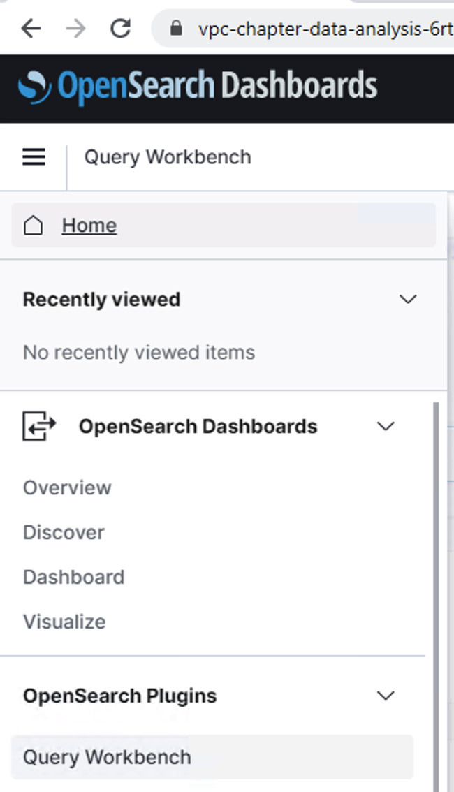
Figure 13.36 – Query Workbench

11. Run the following query in the Query editor window. You will notice that the data is available in OpenSearch to use:

    select * from employees order by emp_no;

The following screenshot shows the data:

Figure 13.37 – The results in the Query editor window

In this section, we inserted data from Glue into OpenSearch and then queried it from OpenSearch Dashboards.

Cleaning up

Delete the CloudFormation stack and remove the registration of the S3 location in AWS Lake Formation along with the Data locations permissions that were granted manually for the governed tables part.

Summary

In this chapter, we learned how data in the data lake can be consumed through both Athena and Redshift. Then, we saw how we can create transactional lakes using technologies such as Hudi and Delta Lake. We then checked various mechanisms for consuming streaming sources in Glue using the forEachBatch method and Hudi DeltaStreamer. Finally, we checked how the ElasticSearch connector from the AWS Glue connector offerings can be used to push data into an OpenSearch domain and consumed through OpenSearch Dashboards. This chapter familiarized you with the most common patterns of data analysis and ETL using AWS Glue.

In the next chapter, we will learn about ML. We will find out more about the strengths and weaknesses of SparkML and SageMaker and when to use each of those tools.