
10
Classification Algorithms
A classification is a definition comprising a system of definitions.
Karl Wilhelm Friedrich Schlegel
10.1. Introduction
Linear regression, as we saw in the previous chapter, is used when we want to build a model that predicts a value. But what happens if we want to classify something? In this case, we can use classification algorithms.
These algorithms, which belong to the supervised learning group, appear in applications related to data analysis. These algorithms can be used on structured or unstructured data. They seek to assign class labels to new data-sets or observations based on existing observations.
In other words, these algorithms are a set of techniques and data analysis methods that classify data by identifying the class or category to which new data belongs.
To better explain, let’s look at a simple example. This is the example that we have already mentioned in the previous section. It’s the spam filter that can learn to report spam using other examples of spam that contain unreliable terms such as “money transfer”, or that come from senders not in the recipient’s contact list.
Based on an email’s contents, messaging providers use classification to determine if incoming email messages are spam (Androutsopoulos et al. 2000; Sedkaoui 2018a). Classifications algorithms will, depending on the data-set, which are also called “training sets”, mark spam in incoming emails. They classify emails based on experience, corresponding to the training data.
So unlike regression analysis, which seeks to predict a value based on previous observations, classification predicts the category to which the new data-sets may belong. It is a set of techniques for determining and classifying a set of observations or data (Sedkaoui and Khelfaoui 2019).
Classification techniques begin with a set of observations to determine how the attributes of these observations may contribute to the classification of future observations. Classification techniques are widely used for prediction purposes. They are useful for customer segmentation, the categorization of audio and images, and the analysis of text and customer sentiment analysis, etc.
If you want to look at such problems by applying unsupervised algorithms for your project, consider algorithms such as decision trees, k-Nearest Neighbors (kNN), Support Vector Machine (SVM), neural networks, Naïve Bayes, Random Forest, etc. It should also be noted that logistic regression, which we have previously discussed, is also one of the most common methods of classification.
In this chapter, we’ll focus mainly on the different methods relevant to a use case from the sharing economy context. We will study a variety of classification algorithms that you can use to analyze large datasets. By opening these algorithms’ black boxes, this chapter will help you better understand how they work.
10.2. A tour of classification algorithms
Classification is a Machine Learning technique that uses known data to determine how to classify new data in a set of existing categories. This technique includes a set of algorithms that we can use to determine how the new data should be classified under a set of labels, classes, or categories using known data.
In this part of this chapter, we will go through a selection of classification algorithms commonly used in data analysis. This will allow you to learn the differences between classification algorithms and to develop an intuitive understanding of their applications.
10.2.1. Decision trees
Decision trees, also called “prediction trees”, use a tree to specify sequences of decisions and their consequences. Given the attributes of observations and classes, the decision tree produces a sequence of rules can be used to classify data. This algorithm is based on a graphical model (trees) to determine the final decision. Their goal is to explain a value from a set of variables.
This is the classic case of a matrix X with m observations and n variables associated with value Y to be explained. The decision tree thus builds classification or regression models in tree form.
Classification models are generally applicable to categorical types of output variables, such as “yes” and “no”, “true” and “false”, etc. However, regression models can be applied to discrete or continuous output variables, such as the expected price of a service (an apartment) or the probability that a subscription will be requested.
This algorithm can be applied to various situations, and its visual presentation helps to break down a set of data into subsets while incrementally developing an associated decision tree. Given its flexibility and that its corresponding decision rules are fairly simple, this algorithm is frequently used in Big Data analysis.
10.2.1.1. The structure of the decision tree
Decision trees use a graph structure in which each potential decision creates a new node, which results in a graph similar to a tree (Quinlan 1986). Each node has a state, and connections are based on this state. The further we descend into the structure, or down the tree, the more these states are combined.
In other words, a decision tree uses a tree structure to represent a number of possible decision paths and a result for each path. To better understand this structure, we’ll use an example that will help us predict whether a proposed service platform will interest people.

Figure 10.1. Example of a decision tree
We can see in Figure 10.1 that the tree acts like a flowchart.
A decision tree is a classification algorithm that uses tree-like data structures to model decisions and results. The structure of this algorithm is as follows:
- – Nodes, or branching points, which are often called “decision nodes”. They usually represent a conditional test. These nodes are the decision or test points. Each node refers to an input variable or an attribute. Each tree starts with a root node where the most significant attribute for all the observations is located (gender, in our case).
- – The branch represents the result of each decision and connects two nodes. Depending on the nature of the variable, each branch makes it possible to visualize the decision’s state. If the variable is quantitative (numerical), we place the upper branch to the right. We may include certain components (equal, less, etc.).
- – Leaf nodes indicate the final result (interested in this service or not). They represent class labels in classification problems, or a discrete value in regression problems.
Note that the depth of a tree is the minimum number of steps required to achieve the result from the root. In our example, the “age” and “income” nodes are one step from the root, and the four nodes at the bottom are the result of all previous decisions. From the root to the leaf lie a series of decisions taken at various internal nodes.
10.2.1.2. How the algorithm works
The purpose of a decision tree is generally to build a tree T from a set of observations S. If all S observations belong to a class C, “gender: male” in our example, then the node is regarded as a leaf node and receives the label C.
However, if any S observations do not belong to the class C, or if S is not pure enough, the algorithm selects the next most informative attribute (age, etc.), and the S scores based on the values of this attribute. Therefore, the algorithm builds subtrees (T1, T2, etc.) for subsets of S, recursively, until one of the preceding criteria is fulfilled.
The first step is to select the most informative attribute. A common way to identify this attribute is to use methods based on entropy (Quinlan 1993). These methods select the most informative attribute based on:
- – entropy: shows the uncertainty of the randomness of the elements or, in other words, a measure of the impurity of an attribute. Entropy measures the homogeneity of a sample. If the sample is completely homogeneous, entropy is zero, and if it is divided equally, it means that it has an entropy equal to one. Either a class X and its label x ∈ X or P(x) the probability of x. Hx, the entropy of X is defined as follows:

- – information gain: this measures the relative change in entropy in relation to the independent attribute. It tries to estimate the information contained in each attribute. Information gain therefore measures the purity of an attribute. To build a decision tree, we must find the attribute that returns the highest information gain (that is to say, the most homogeneous branches). Information gain assigns a class for filtering on a given node of the tree. Classification is based on the entropy of the information gain in each division. The information gain of an attribute A is defined as the difference between the base entropy and the conditional entropy of the attribute:
10.2.2. Naïve Bayes
The Naïve Bayes algorithm is a set of classification algorithms based on Bayes’ theorem. This is not a single algorithm, but a family of algorithms that share a common principle, that is to say that each pair of features is classified independently from each other. To help you understand the principle of this algorithm, we will look at its different applications.
10.2.2.1. The applications of the algorithm
Naïve Bayes is a fairly intuitive classification algorithm to understand. A classification using this algorithm assumes that the presence or absence of a particular characteristic of a class is not related to the presence or absence of other features. For example, an object can be classified according to its attributes such as shape, color, and weight.
It can be used for binary and multiclass classification problems. The main point is the idea of treating each feature independently.
The Naïve Bayes method assesses the probability of each entity independently, irrespective of any correlation, and determines the prediction based on Bayes’ theorem (Sedkaoui 2018b).
Using this method has the following advantages: simplicity and ease of understanding. Moreover, this algorithm generally performs well in terms of resources consumed, since only the probabilities of the characteristics and classes must be calculated; it is not necessary to find the coefficients as in other algorithms.
Because Naïve Bayes is easy to implement and can be run efficiently, even without prior knowledge of the data, it is one of the most popular algorithms for classification of textual data.
Besides its simplicity, this algorithm is also a good choice when CPU and memory resources are limiting factors.
This classification algorithm can be used in real-world applications such as:
- – sentiment analysis and text classification;
- – filtering unwanted messages (spam);
- – recommendation systems;
- – facial recognition;
- – fraud detection;
- – real-time predictions;
- – predicting the probability of several classes for the target variable.
Its main drawback is that each feature is treated independently, even though in most cases this cannot be accurate (Bishop 2006).
10.2.2.2. Operation of the Naïve Bayes algorithm
Naïve Bayes is a classification technique based on Bayes’ theorem that assumes independence between the predictors. That is to say, it assumes that the presence of an entity in a class is not linked to any other entity. Although these features are dependent on each other or on the existence of other features, all of these properties are independent.
This theorem can be extended to become a Naïve Bayes classifier. First, we can use the conditional independence hypothesis, which states that each attribute is conditionally independent of any other attribute given the label of class Ci:

Therefore, this assumption simplifies the calculation of P(a1, a2,…, am/ Ci).
Then, we can ignore the denominator P(a1, a2,…, am), since it appears in P(Ci/Ai) (for i = 1, 2 … n); removing the denominator will have no impact on the relative probability scores and will simplify the calculations.
Here, Ai represents the attributes or characteristics, and C' is the response variable. Now, P(Ci/Ai) becomes equal to the product of the probability distribution for each attribute X.
We are interested in finding the probability P(Ci/Ai). Now, for several values of C, we will calculate the probability for each of them.
So how do we predict the class of the response variable as a function of the different values that we obtain for P(Ci/Ai) ? We simply take the most likely or the maximum of these values. Therefore, this procedure is also known as “maximum a posteriori estimation”.
10.2.3. Support Vector Machine (SVM)
Unlike regression, which can be regarded as a sword that is capable of slicing and dicing data efficiently but is unable to process highly complex data, “SVM” is like a sharp knife that works on smaller data-sets but can be much more powerful for building models based on these data-sets.
We assume that you are already accustomed to the algorithms of linear regression and logistic regression. If not, we suggest that you reread Chapter 9 before moving on to the Support Vector Machine algorithm (SVM).
A Support Vector Machine is another simple algorithm that produces accuracy results with less computing power (Cristianini and Shawe-Taylor 2000). SVM can be used both for regression and classification tasks, but it is especially widely used in classification.
10.2.3.1. Definition of SVM
A Support Vector Machine is an algorithm that seeks to divide the hyperplane with the widest possible gap to improve resistance to noise. Like logistic regression, it is a discriminating method that focuses only on predictions.
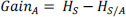
This is a classification method, in which we include each data point in a dimensional space n (where n is the number of entities) and the value of each entity is the value of a particular coordinate. Then, the classification is done by searching the hyperplane, which clearly differentiates the two classes.
For example, if we have only two variables, such as renting an apartment or a villa on Airbnb, we must first draw the two variables in a two-dimensional space (n = 2), with each point having two coordinates called support vectors (see Figure 10.2 for more detail).
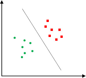
Figure 10.2. Coordinates of entities divided into two classes. For a color version of this figure, see www.iste.co.uk/sedkaoui/economy.zip
Now let’s look for a line that divides the data between the two groups of differently classified data, knowing that the distance of the nearest point for each group will be those farthest away.
So, in SVM, the goal of optimization is to maximize “the gap”. This gap represents the distance between the separating hyperplane and the nearest points of this hyperplane, called support vectors.
The question that now arises is: “How do we identify the right hyperplane?”
10.2.3.2. SVM: how it works
In Figure 10.2, the line that divides the data into two different classes is the black line, because the two closest points are farthest from that line. Then, as a function of the data’s location on one hand and the line on the other, we can classify new data.
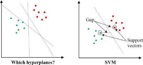
Figure 10.3. How SVM works. For a color version of this figure, see www.iste.co.uk/sedkaoui/economy.zip
As shown in Figure 10.3, there are several ways to separate the data. To resolve this issue, SVM seeks the best line separating the data by maximizing the orthogonal distance between the nearest points of each data category and the limit of the line.
Distances called “gaps”, and the points used to define the gap (the nearest boundary points) are called “support vectors”. Once the ideal function is determined, the algorithm is able to predict whether people prefer to rent an apartment or a villa.
This example illustrates the application of this algorithm and shows a linear hyperplane between these two classes or groups. SVM can effectively perform linear classifications and can also be configured to perform nonlinear classifications (Cristianini and Shawe-Taylor 2000).
10.2.4. Other classification algorithms
In addition to the three classification algorithms presented above, several other algorithms are also used to analyze large amounts of various kinds of data. In particular, these include k nearest neighbors (kNN), random forest and neural networks. These algorithms are commonly used methods for obtaining the best models.
10.2.4.1. The k-nearest neighbors (kNN)
The kNN, or k-Nearest Neighbors is an algorithm that can be used both for classification and regression. The principle of this model is to choose the k closest data points under study to predict its value (Sedkaoui 2018b). In classification or regression, the input will consist of the k closest training examples in a space.
To understand how this algorithm works, let’s consider a small visual example that will help you understand this algorithm. In Figure 10.4, we have two classes of data, red circles and black squares. It should be noted that the input is two-dimensional and the target to be classified is the shape.

Figure 10.4. How does kNN work?. For a color version of this figure, see www.iste.co.uk/sedkaoui/economy.zip
Suppose now that we have a new input object whose class we want to predict. How should we proceed? Well, let’s consider the k nearest neighbors to this object and see which class contains the majority of these points in order to deduce its class.
In this example, we used 5-NN (k = 5), and we can say that the new entry belongs to the class of red circles, as its nearest neighbors contain three (3) red circles and two (2) black squares.
The principle of this algorithm is to assign a set of data to one of the class categories by calculating the distance separating it from each point in the data-set. We choose the first k elements in the series of distances and therefore choose the dominant label from among the k elements, which represents the category of the element in the data-set.
10.2.4.2. Random Forest
Random Forest is one of the most popular supervised learning algorithms. It requires virtually no preparation or data modeling and usually provides accurate results (Sedkaoui 2018a). Random forests are based on the decision trees described above.
More specifically, random forests are collections of decision trees (Breiman 2001) that produce a better forecast. This is why it is called a “forest” (or set of decision trees).
So, as the name suggests, this algorithm creates a forest and renders it somewhat random. This forest constitutes a set of decision trees, generally trained with the bagging method (Breiman 1996).
Random Forest develops several trees into a model. To classify a new object or a new entry in terms of new attributes, each tree provides a classification, and we say that this tree “votes” for this class. The forest chooses classifications with the most votes among all the trees in the forest and takes the average difference of the production of different trees.
This algorithm therefore builds several trees and combines them to get a more accurate result.
10.2.4.3. Neural networks
Neural networks are inspired by the neurons in the human nervous system. They help find complex patterns in the data. These neural networks learn a specific task as a function of the data-set (Sedkaoui 2018b).
Thanks to recently developed Deep Learning algorithms, neural networks have been developed as a method for facilitating a number of complex tasks such as image classification, voice recognition, etc.
In neural networks, we have an input layer that receives the input data and then propagates the data to the hidden layers. Finally, the output layer produces the classification result.
Each tier of the neural network is a set of interconnections between the nodes of a tier with those in the other tiers. So, neural networks consist of nodes (Figure 10.5).

Figure 10.5. Example neural network
So, we’ve taken the tour of the different classification algorithms. We found that each algorithm has its own properties. But to help you identify the most suitable method for a specific problem, we suggest, in Table 10.1, a list of items to consider.
Depending on the set of training data and the variables, we will opt for one of these algorithms. The goal is the same: to predict or classify new entries. For example, to determine whether a new email is spam or not.
Now let’s examine the theory behind these classification algorithms and use an example from the sharing economy to explain how these methods work in practice, while continuing to explore how Big Data analytics can be used to generate value for companies in this economy.
Table 10.1. How do we choose the classification algorithm?
|
Questions |
Algorithms |
|
Should we include the class of the classification? How can the variables affect the models? Are some of the input variables correlated? Does the data contain several types of variables? |
Logistic regression |
|
Are certain input variables relevant? Does the data contain categorical variables with many levels? |
Logistic regression |
|
Is the data high dimensional? |
Naïve Bayes |
|
Is there nonlinear data or discontinuities in the input variables that can influence the outcome? Is it an interoperability problem? |
Decision tree |
|
Is the goal to predict the probability of a particular event? |
Logistic regression |
|
Can the linear model be extended to nonlinear problems? |
SVM |
|
How can we make predictions without a training model, but with a more expensive prediction step in terms of processing? |
kNN |
|
Are we looking for complex models in the data? |
Neural Networks |
10.3. Modeling Airbnb prices with classification algorithms
Are some factors more important in terms of generating higher rates?
To answer this question, we’ll use what we already have to model and predict the price of Airbnb apartments in Paris from the set of observed data.
In this section, therefore, we’ll reexamine the example from Chapter 9 to better show you how different classification algorithms can be used. But first, we think it’s important to review the various steps of the process we have adopted.
10.3.1. The work that’s already been done: overview
We started with data preparation and processing to make it more consistent and to eliminate missing and non-significant values (NAN).
Next, we performed an exploratory analysis to identify the most significant variables that can best explain the model. This analysis allowed us to discover the importance of some attributes, such as: bedrooms, neighborhood, room_type, etc., and how they can influence prices.
Therefore, after analyzing all the results, it was determined that 20 variables are the most significant for the model. These variables will serve in this chapter as a reference for comparing the results of different models.
These steps represent the key that helped us exploit 58,740 observations. Using different techniques, exploratory analysis allowed us to advance step by step to understand the most important variables before running the regression models (linear, Ridge and Lasso).
The results of the regression technique applied in Chapter 9 argue in favor of the assumption that the prices of apartments are higher if they are close to the center of Paris and if they have necessary equipment (beds, bathrooms, etc.) in addition, of course, to its condition (type of housing, property, etc.).
A linear model was created by measuring the price compared to 20 variables that were measured at the 0.001 level. The RMSE, measured at 2368.596, was higher than the ideal. This means that the expected price for a rental can vary by 2368.596 euros when compared to the real rental price. Linear regression therefore generated the worst performance.
Two other models were used, Ridge and Lasso, to solve the problem of highly correlated independent variables. Both models had relatively similar test scores. But the performance of Ridge was better than Lasso, and the model didn’t overadjust too much in relation to the training set. Ridge regression allows for better price predictions for Airbnb apartments.
Now, we will also try other algorithms that make it possible to better predict prices. We will use Random Forest and a decision tree to determine the characteristics that are more important for determining the prices of Airbnb apartments in the French capital.
10.3.2. Models based on trees: decision tree versus Random Forest
Since our database is ready, having been prepared and analyzed in Chapter 9 of this book, we can begin with the modeling phase using the algorithms we have discussed in this chapter. The objective is to continue seeking a model that can best present our data and enable prediction of the value of the results, or the price of Airbnb apartments in Paris.
As you have seen in the previous sections of this chapter, there are several algorithms that we can take advantage of to build the model. But we’re going to use two of them: decision tree and random forest.
10.3.2.1. Decision trees
As we indicated at the beginning of this chapter, decision tree refers to types of classification algorithms that have a predefined target variable.
This algorithm is mainly used for classification but can also be applied to prediction problems with both categorical and numerical variables.
Tree models can capture non-linear relationships in sets of observations. Using a tree structure, a decision tree comprises a plurality of internal nodes, each of which corresponds to a characteristic (e.g. the number of rooms), and each decision node is a class label (e.g. the number of rooms is less than or greater than 2).
Now we’ll adjust the decision tree algorithm for our listings.csv data. But before doing this in Python, we need to import certain required libraries, such as:
- – NumPy and pandas: for manipulating data;
- – train_test_split from cross_validation: for splitting the data into a train (x_train, y_train) and a testing (x_test, y_test) set;
- – DecisionTreeClassifier: for creating a decision tree classifier;
- – Accuracy_score: for calculating precision metrics from the variables of the predicted classes.
To understand the performance of the model, we divided the data-set into a train set and a test set using the train_test_split function. The test_size parameter has a value of 0.3; this means that the test sets will account for 30% of all data, and the training data-set will represent 70% of the data.
The random_state variable is a state generator for pseudo-random numbers used for random sampling.

The decision tree algorithm used for classification problems (like the one we are currently examining) aims to create one of these decision trees in order to assign records to a defined number of categories.

Figure 10.6. The 10 most important features (decision tree). For a color version of this figure, see www.iste.co.uk/sedkaoui/economy.zip
Having trained the decision tree model (with the train function) to classify characteristics according to their importance, we are now able to determine what features have greater weight in the calculation of prices. The results of this classification are illustrated in Figure 10.6.
Drawing a conclusion from this model, we can see that the algorithm has identified amenities and location as the main contributors to the way in which it predicted prices. We found that the most important features were:
- – longitude;
- – host_total_listings_count;
- – latitude;
- – accomodates;
- – bedrooms;
- – bathrooms.
Other features (Elysée, etc.) concerning the apartment’s location.
The question that you may now be asking is: how do we select the criteria and values for classification? It is the intelligence of the algorithm that does it for you; the principle is simple: start with the most discriminating variables, that is to say that we must create the greatest possible level of disorder, a principle that is mathematically modeled by the entropy function (Sedkaoui 2018b).
Using the data-set, we calculated the RMSE, which is equal to 21.505. What we can see from this value is that it is very high compared to the RMSE values for the Ridge (14.832) and Lasso (15.214) regressions.
These characteristics gain more weight because they tend to be more linearly correlated. Those whose correlation coefficient was higher tended to increase apartment prices.
As can be seen in the resulting graph, the decision tree captures the general trend of the data. However, one disadvantage of this model is that it does not account for the continuity and differentiability of the desired prediction. In addition, we must make sure we select an appropriate value for the tree depth to avoid over-or under-adjusting the data.
We will use the Random Forest algorithm to process the data.
10.3.2.2. Modeling using Random Forest
We chose the Random Forest model because this model uses a blending technique that combining several models into one. This method usually reduces the variance and bias in observational data, which improves forecast accuracy.
The advantage of the Random Forest algorithm is independence between the trees, which makes it possible to parallelize processing and improve the algorithm’s performance. Every tree is different, and their grouping should make it possible to achieve a lower degree of variance than a single tree.
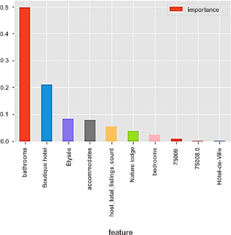
Figure 10.7. The 10 most important features (Random Forest). For a color version of this figure, see www.iste.co.uk/sedkaoui/economy.zip
With regard to our example, we first used the data-set to train the model by applying the Random Forest algorithm. We then used the test data-set to test this model and proceed to validation. This allowed us to determine the most important features, which include two factors (equipment/location).
Among the features shown in Figure 10.7, we can identify a set of important variables, which include:
- – bathrooms;
- – accomodates;
- – host_total_listings_count;
- – bedrooms.
These are almost the same variables as the significant variables in our decision tree model, which shows that they are key predictors for forecasting the prices of Airbnb apartments in Paris.
We obtained an RMSE , equal to 14.775 (Table 10.2), which is lower than the RMSE values of the other models.
Table 10.2. MSE and RMSE for each model
|
Model |
MSE |
RMSE | |
|
Models based on trees |
Decision tree |
462.465 |
21.505 |
|
Random Forest |
218.300 |
14.775 | |
|
Baseline models |
Median |
243.079 |
15.591 |
|
Mean |
243.079 |
15.591 | |
|
Regression model |
Ridge |
219.988 |
14.832 |
|
Linear |
5610218.588 |
2368.59 | |
|
Lasso |
231.465 |
15.214 | |

Figure 10.8. RMSE: score for the different models. For a color version of this figure, see www.iste.co.uk/sedkaoui/economy.zip
Note that since the price distribution is slightly skewed to the right (see Figure 9.8 in Chapter 9), we have added two basic models that could explain this bias by setting average values to 110.78 euros and median values to 80 euros.
By comparing the RMSE values, we see that the linear regression model showed the highest value for RMSE (2368.59) and that the random forest model has the smallest value (14.775). The random forest model surpasses other models in terms of predictive accuracy. Based on the RMSE test for each model, we selected the Random Forest model as the best model for predicting the price, because it has the smallest RMSE.
This model is most effective for predicting Airbnb prices because it is easier to identify important predictors. This algorithm works well with large-scale predictors and large sets of training data. However, the downside is that prediction takes too long when there is a large number of trees.
We also concluded that the most important variables for predicting prices are the variables related to location and amenities (bedroom, bathroom, location, etc.). The total number of guests as well as hospitality play a role, but all the models have shown the significance of the list of amenities, home type, and location.
Based on these findings, we want to predict price using a different algorithm: kNN, because as hosts you would surely consider all factors that affect the price of your apartment; in order to automate the data analysis process, we have been using the k nearest neighbor or kNN algorithm since we began our work.
10.3.3. Price prediction with kNN
We will, in this section, continue our efforts to learn what lies within our large data-set. By using the results of previous algorithms as a basis, we will analyze certain characteristics related to location and equipment that which seem to be very important for determining prices.
We now look for other alternatives by using the kNN algorithm, which is first applied to select the number (similar ads) that we will compare. Then we calculated the similarity in order to classify each list as a function of similarity. Finally, we
calculated the average price for k and considered it as the current price. It should be noted here that we set k to 5.
To calculate the distance, we began with the accommodates variable and then incorporated other variables. The smallest possible Euclidean distance is equal to zero, which would mean that the current observation is similar to ours. The calculation of the Euclidean distance is described in detail in Chapter 11 of this book.
The calculation of the Euclidean distance for each observation in the data-set generated the results presented in Table 10.3.
Table 10.3. Number of observations by distance
|
Distance |
Nbr |
Distance |
Nbr |
Distance |
Nbr |
|
0 |
5938 |
5 |
560 |
10 |
13 |
|
1 |
44093 |
6 |
101 |
11 |
16 |
|
2 |
5279 |
7 |
135 |
12 |
13 |
|
3 |
3156 |
8 |
22 |
13 |
31 |
|
4 |
486 |
9 |
37 |
14 |
1 |
The results show that there are 5,938 observations in the data-set that have a distance equal to 0. This means that these 5,938 observations have welcomed the same number of people.
If we were only using the first five observations that have a distance equal to zero, we might end up with biased predictions. To avoid this problem, we randomized the order of the observations and then selected the first five lines. This allowed us to randomly select the observations mentioned in Table 10.4.
Table 10.4. The price of the first five randomized observations
|
Observation |
Price (EUR) |
|
19843 |
75 |
|
10454 |
99 |
|
17543 |
129 |
|
13622 |
100 |
|
36921 |
120 |
It should be noted here that the results contained certain characters when retrieved, such as the dollar sign ($) and commas. So, we cleaned the data to remove these characters by converting them into a floating type.
Then we calculated the average price of these first five observations, and we got a value that is equal to 104.6 euros. This means that when we use only the accommodates variable to predict prices (with the same number of guests), we must set the price of the apartment to 104.6 euros.
The question that arises now is: how correct is this prediction result?
To answer this question, we evaluated the accuracy of this model. For this, we divided our database into two parts:
- – a train set, which contains half of the observations;
- – a test set, for testing the model of the other half.
What we wanted to do here is to use half of the observations to predict the price and compare this value with the actual price in the data-set to analyze the accuracy of the result.
We also calculated the RMSE of this model, and the value we obtained is equal to 272.59. To better understand the magnitude of this model, we have, at this point, incorporated other variables (bathrooms, bedrooms, longitude, etc.) to create other price predictions. We computed the RMSE of each of these variables and compared them. The results are shown in Table 10.5.
Table 10.5. Comparison of RMSE values for different predictors
|
predictor |
RMSE |
|
Accommodates |
272.59 |
|
Bedrooms |
275.36 |
|
Bathrooms |
276.79 |
|
host_total_listings_count |
287.49 |
You can see, through the results in this table, that the kNN algorithm lets you capture the features that most affect the price. According to the RMSE values, we can say that the best predictor is the one with the smallest RMSE value: accommodates.
So, we have built a model that explains the prices of Airbnb apartments using a single variable (accommodates). We then predicted the price by incorporating several variables at once: this is called a “univariate model”.
Our goal was not only to choose a model that best represents all of our data, but also to show you the power of analytics and what we can do with the various algorithms.
For more results, you can try the various techniques we have discussed in this chapter (Naïve Bayes, SVM, and neural networks). Then you need to select the most appropriate model that allows you to make predictions based on the characteristics of the data-set and predictors or variables, and, of course, the prediction goal you want to achieve.
Indeed, it is important to see how companies can understand their data, how to handle missing variables, create an explanatory model, make a decision tree, etc. that will enable them to understand and form their own analytics instruction manual for working with large data-sets, or Big Data.
10.4. Conclusion
In this chapter, you learned about several Machine Learning algorithms and their different uses for solving classification problems and even regression. We found that these algorithms are used for various applications. This chapter, in fact, examined the theory behind the various classification algorithms and used an example of a sharing economy company to explain how these methods work in the business world.
Using this example, which is the same one we used in the previous chapter, we conducted tests using two classification algorithms: decision tree and Random Forest. The results allowed us to compare the different models and choose the best. Based on the RMSE value, the most reliable model was Random Forest.
We applied the k-nearest neighbors algorithm to create a univariate predictive model. The results show that we can use other variables to improve the prediction.
This fun little data analysis project is a crucial passage for anyone who wants to work with Big Data. This is a very easy data-set, but even if you think that predicting prices for Airbnb apartments is a problem that does not interest you, examples like this allow you to apply different methods and algorithms for supervised learning, pending our discussion of unsupervised algorithms (cluster analysis) which will be the topic of the next chapter.
The quantity and variety of data produced today is a big advantage for sharing economy companies. Developing a data analysis process is therefore essential to creating value. This example is only one of many use cases, because data analysis methods can be applied in different circumstances that require model identification or prediction.
These tests and analyses are only part of what supervised learning algorithms (regression and classification) can allow sharing economy companies to do. If software makes it possible to project or to model the past in order to develop scenarios for the future, then Big Data represents a step forward by modeling the future to make good decisions possible today.
TO REMEMBER. This chapter provided the opportunity to learn that:
- – classification is an approach for classifying new observations from historical observations;
- – classification algorithms are varied, can be applied to large data-sets, and can make it possible to classify data into groups and to identify the class or category to which a new data point belongs.
In addition to decision trees, Naïve Bayes, and SVM, other algorithms are commonly used for both classification and regression, such as kNN, Random Forest and neural networks.