
5
Mobile Cloud Networking and Mobility Control
Mobile Cloud Networking (MCN) is a solution which has become very important in the context of mobile networks. The basic element is the mobile terminal, which moves around and requests services from a Cloud which, for its part, is fixed. Mobile Cloud also refers to technologies where the Cloud itself is mobile. It moves around with the client. The mobile Cloud may be virtual but also physical. We shall begin, in the first section, by examining MCN, and then in the second section we shall look at mobile Clouds, before concluding this chapter with a discussion of the means of control of mobility of the terminals and users.
5.1. Mobile Cloud Networking
The exact definition of “Mobile Cloud Networking” is very controversial, because there is no real definition and no clear architecture. There are two predominant orientations in the field of MCN:
- – an application orientation, which means that a mobile device with limited resources is able to handle applications which require intensive computations or more memory than the terminal has;
- – a network orientation, which involves the optimization of algorithms for the control of mobile services.
In the context of application orientation, we can cite various applications which correspond to this framework, such as Rich Mobile applications, “Mobile Cloud gaming” or indeed MGaaS (Mobile Game as a Service), augmented reality or mobile applications involving intensive computations such as OCR (Optical Character Recognition) or natural language use.
In the context of network orientation, we might find, for example, firewalls for mobile devices, handover control or the management of mobile terminal attachment.
The architectures for “Mobile Cloud Networking” cover the different classifications mentioned above: Cloud networking for mobile terminals, local Clouds, virtual Clouds or indeed Cloudlets. The first architecture is illustrated in Figure 5.1.

Figure 5.1. An architecture for Mobile Cloud Networking
This architecture shows a mobile terminal – a smartphone – which uses a central Cloud to handle a certain number of applications. These applications are CPU intensive, a very high memory requirement or the use of specific resources which cannot be accommodated on the smartphone as a “big data” depository. The communications between the smartphone and the Cloud must be reasonable so that the wireless interface can handle them without any problems. In summary, the terminal is a lightweight machine which calls on the Cloud to carry out hungry processes.
Figure 5.2 illustrates the second architecture, which is fairly similar to the previous one but where the Cloud is no longer central, but is local, or at least not too far from the user. The resources can be hosted on other mobile devices that are connected to the Cloud. The mobile devices may themselves form a Cloud. In other words, neighboring mobile terminals, if they are inactive, can perfectly well serve to perform a computation, storage, or even a network in that environment. We shall see these scenarios for Mobile Cloud at the end of this chapter.

Figure 5.2. An architecture for local Mobile Cloud Networking
This “Mobile Cloud” is built from connected machines and possibly a local datacenter, which may be very local with micro-datacenters or nano-datacenters or pico-datacenters or even femto-datacenters. Overall, the small datacenter can be situated at the level of the DSLAM of the access router or even the Home Gateway.
Figure 5.3 presents a third case of MCN with a virtual Cloud. In this solution, the client with his/her mobile device wishes to connect to a whole set of Clouds to cover all the services he/she requires. As a single Cloud is usually insufficient to contain all the services necessary for a user, the user needs to request connection to several Cloud providers to obtain the services he/she needs. As it may be tricky and complex to know all the solutions, one possibility is to call on an intermediary which has extensive knowledge of all the Clouds. This intermediary is able, at any given time, to choose the best possible Cloud provider for a given application. The Cloud is virtual because it is represented by an intermediary virtual machine capable of connecting the client to the best Cloud to deliver the required application. Another name given to this solution is “Sky”, and the intermediary is a Sky provider. One of the difficulties for the Sky provider is intermediation with Clouds which may be very different to one another, but which must not appear any differently to the end user.

Figure 5.3. A third Mobile Cloud Networking architecture
Finally, the fourth architecture encountered under the auspices of Mobile Cloud Networking also pertains to the use of a small Cloud – a Cloudlet – which moves with the client. In fact, it is not that the Cloud actually moves, but the connection to different Cloudlets gives the impression that the Cloud is moving with the client. With each handover, the mobile terminal attaches to a new Cloudlet, and the client’s virtual machines migrate over to the new small datacenter. This solution is illustrated by Figure 5.4.

Figure 5.4. A fourth architecture for Mobile Cloud Networking
A Cloudlet is a concept of a small Cloud situated in a zone with very high demand. The Mobile Cloud provider assigns the most appropriate Cloudlet to respond quickly to the service request of the moving client.
In summary, Mobile Cloud Networking architectures are based on a hierarchy of Clouds to optimize different criteria:
- – performance and reliability of applications for mobiles;
- – performance of control applications for mobiles;
- – minimization of energy consumption by the terminals, datacenters, etc.;
- – availability;
- – high security:
- - m-commerce,
- - m-Cloud access,
- - m-payment.
The architectural differences we have described can be combined to optimize the above criteria. Once again, we see the hierarchy of datacenters ranging from enormous datacenters to the minuscule “femto-datacenters”. It is not easy to optimize these environments, even though the architecture is sometimes relatively well defined. Often, it appears that the system of the future is Clouds that form easily and are just as easily transformed, and is beginning to gain momentum, known by the name “mobile Cloud”, which we shall now examine.
5.2. Mobile Clouds
A “mobile Cloud” is a set of small datacenters which, once they are connected, form a Cloud. The difficulty lies in the mobility of such Cloudlets and the diversity of forms of mobility, so the Cloudlets can attach and detach. If all the Cloudlets or mini-datacenters move simultaneously, then it is a VANET (Vehicular Area Network) which supports the mobile Cloud. On the other hand, if the mobiles which transport the mini-datacenters move independently of one another, with no coordination between them, the mobile Cloud has greater difficulty in forming and evolving on the basis of the movements. Figure 5.5 shows an example of a mobile Cloud, wherein each vehicle has its own femto-datacenter.
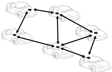
Figure 5.5. Example of a mobile Cloud
Communications between datacenters take place by way of a mesh or ad-hoc network. An ad-hoc network occurs in the case where the femto-datacenters are hosted on the same device as the communication port with the other machines possessing datacenters. In the case of a mesh network, there is a specific network which forms the link between the femto-datacenters. This network has nodes with two communication ports: one to connect with the clients and femto-datacenters, and the other with the nodes of the mesh network.
In the case of a mesh network, the vehicle has a box entirely devoted to inter-vehicle communication. The devices in the vehicle – “things”, objects or any other piece of equipment – are connected to the mesh box. As we have seen, the box has two communication ports: one for connecting devices inside or outside the vehicle, and a second for communication between different boxes. The second solution – ad-hoc networks – can be used to form direct connections between the objects or other equipment. This solution is not advocated by operators, because the user’s device needs to include networking equipment to perform communication. In addition, user applications, running on the same machine, may interfere with this equipment.
An example of a mobile Cloud is shown in Figure 5.6, where all the vehicles are traveling at approximately the same speed, which enables the Cloudlets to simply connect with one another at acceptable speeds to form a wider Cloud. In fact, there are two mobile Clouds: one for each direction of travel of the vehicles.

Figure 5.6. Two mobile Clouds
A large mobile Cloud can be established when a traffic jam occurs, as shown in Figure 5.7. When hundreds of vehicles are in the same place, the overall power may become quite substantial. The vehicles must be connected in a mesh network with specific protocols, such as OLSR, to allow for data transmission between the vehicles.
5.3. Mobility control
Mobility is difficult to manage because the decisions essentially need to be made in real time, and the motion means that it is impossible to use powerful entities such as datacenters, which are situated too far from the periphery, except perhaps if we consider new technologies such as C-RAN, where the local loop needs to be rethought, and replaced by an optical network. With few exceptions, we must move the decisions to the endpoints, and this delocalization is done by local controllers. We again see the issue of SDN on the periphery, which we have already touched on many times. The OpenFlow protocol may play an important role in connecting the client and the controller.

Figure 5.7. A large mobile Cloud
Two types of controller may be found, low-level controllers and high-level controllers. The former handle the lower layers: frequency regulation, power regulation and adaptations of the physical and link layers – i.e. of levels 1 and 2. These controllers can also manage certain types of security applications, such as detecting hacker access points. High-level controllers are associated with SDN controllers. They are capable of handling the properties shown in Figure 5.8.
These properties contain the authentication of users by any given technique, with the harvesting of a maximal number of characteristics of the user and his/her applications. The reason for this information-harvesting is to facilitate an SDN control performed directly by the local controller or to transmit these data to a central SDN controller. The user’s characteristics are often coupled with a database which is regularly updated.

Figure 5.8. Properties of mobile device controllers
The second major property is to determine the user profile, either by harvesting information when authenticating, or by associating the user with a pre-defined profile. This profile enables us to determine the applications which can be run, and thus facilitate access control depending on the user’s demands. For example, the user profile indicates whether or not s/he has access to the Internet solely via HTTP, has the right to use VoIP services, send e-mail, use a local printer, etc.
The third property of controllers pertains to the management and control of flows by using a protocol such as OpenFlow, or another, more conventional, protocol. The controller must also be capable of satisfying the obligatory demands of states, such as storing the logs of clients who connect to the controller.
The last two sets of properties pertain to the management of the connection, firstly by providing the elements necessary to perform a “zero configuration”: the controller is capable of substituting the mobile terminal to provide particular properties. For example, the controller can intercept a user’s electronic messages and send them using its own SMTP, in the knowledge that the network to which the mobile is connected does not accept the messages of the user who is a guest of the company. Another example is the use of a printer from a mobile phone. The controller can load a virtual driver and enable the mobile to print locally. Finally, the controller can manage solutions to enable the user to use passwords to connect to the access point.
If we examine the authentication more specifically, the most conventional method is a window in which the client enters his/her username and password, using the IEEE 802.1x standard, for example. Another solution is access by authentication on another site, such as Google or Facebook, or on a payment server. Once the external authentication has been performed, a specific protocol such as OAuth can send the authentication back to the controller. One final solution may be to ask the user to fill out an information page in order to gain access.
It should be noted that in the last two scenarios, the client must be able to connect to the network without authentication. Thus, the access point must allow him/her to pass on a specific, provisional authorization of the controller. This solution is often an option in authentication systems. However, it is somewhat risky, because once he/she is authenticated on an external server, the client can continue to navigate without returning for a firm authentication on the local controller.
Figure 5.9 presents the two solutions for application controllers: the first is physical and the second virtual. The advantage of the virtual controller is that it uses the resources which are necessary at any given moment – i.e. a great deal of resources at peak times and practically no resources during trough periods.

Figure 5.9. The two controller solutions
Figure 5.10 illustrates the different ways in which it is possible to obtain Internet access authorization using an access point and an access-point controller. Case 1 corresponds to client access to an external authentication site. He/she obtains provisional authorization to pass the access point and seek authentication or recognition on an external site which may be located anywhere on the Internet. Once this authentication has been performed, it is transmitted back to the controller, which sends the order to the access point to allow the client to pass.
Case 2 is that which facilitates a solution with an SDN controller. When a flow comes in, the SDN access point sends a request to the SDN controller, which begins by authenticating the client on a captive portal or using another authentication solution. Once authentication has been completed, the controller grants authorization to the access point, specifying which flow is to be allowed through. The client can then access the Internet.
Case 3 is that of a local physical controller which, after local authentication, allows the client to communicate with the Internet via the access point. The IEEE 802.1x protocol can easily be used in this situation.
Case 4 represents the solution where we need to access the central controller which, after authentication and consultation of the profile, allows the client to access the Internet.

Figure 5.10. Access authorization cases for a controller
5.4. Mobility protocols
The convergence of landline and mobile telephones means that any application installed on a server can be used from a fixed or mobile device. The first condition to achieve this convergence is that a mobile be able to remain connected to the network whilst moving around, without the functioning of the application being interrupted. Changes of cell (known as handovers) must take place transparently and seamlessly, with the same quality of service being maintained if the application requires it.
We shall begin by discussing macromobility, which involves the management of mobility of terminals between two different IP domains, and micromobility, which relates to the change of attachment point within the same IP domain. In the first case, the main protocol is IP Mobile; in the second, various protocols are in competition with one another. We shall then go on to examine multihoming – i.e. the case where a terminal is simultaneously connected to several networks.
5.5. Mobility control
Two main types of mobility control solutions in IP networks have been put in place, depending on the mobile terminal’s movement: support for macromobility and support for micromobility.
In the former case, the mobile changes the IP network, whereas in the latter, it stays within the same network but changes its attachment antenna. Macromobility is handled by the IP Mobile protocol. For micromobility, numerous protocols have been defined. We shall examine the main ones in this chapter.
5.5.1. IP Mobile
IP is increasingly being presented as a solution to the problems posed by mobile users. The IP Mobile protocol can be used in IPv4, but the potential lack of addresses complicates the management of communication with the mobile. IPv6 is preferable, because of the large number of available addresses, which means that temporary addresses can be assigned to the stations as they move around.
The operation of IP Mobile is as follows:
- – a station has a base address, with an agent attached to it, whose role is to monitor the match between the base address and the temporary address;
- – when a call comes into the mobile station, the request is sent to the database in which the base address is held;
- – because of the agent, it is possible to match the base address to the provisional address and send the connection request to the mobile.
This solution is similar to that used in mobile networks.
The terminology employed in IP Mobile is as follows:
- – Mobile Node: terminal or router which changes its attachment point from one sub-network to another;
- – Home Agent: router of the sub-network with which the mobile node is registered;
- – Foreign Agent: router of the sub-network being visited by the mobile node.
The IP Mobile environment is formed of three relatively separate functions:
- – agent Discovery: when the mobile arrives in a sub-network, it searches for an agent capable of handling it;
- – registration: when a mobile is outside of its home domain, it registers its new address (Care-of-Address) with its Home Agent. Depending on the technique used, registration may take place directly with the Home Agent, or be done through the Foreign Agent;
- – tunneling: when a mobile is outside of its home sub-network, the packets need to be delivered to it by way of the technique of tunneling, which links the Home Agent to the Care-of-Address.
Figures 5.11 and 5.12 illustrate the arrangement of communication in IP Mobile for IPv4 and IPv6.
5.5.2. Solutions for micromobility
Various protocols have been put forward by the IETF for the management of micromobility in order to improve IP Mobile. Indeed, micromobility solutions are primarily intended to reduce the signaling messages and the latency of handover caused by the mechanisms of IP Mobile. Generally, we distinguish two categories of approaches for micromobility: those which are based on tunnels and those which use forwarding tables.

Figure 5.11. IP Mobile for IPv4

Figure 5.12. IP Mobile for IPv6
Tunnel-based approaches use local and hierarchical registration. For this purpose, they use IDMP (Intra-Domain Mobility Management Protocol), HMIPv6 (Hierarchical MIPv6) and FMIPv6 (Fast MIPv6).
HMIPv6 is a hierarchical arrangement which differentiates local mobility from global mobility. Its advantages are the improvement of handover performances, because local handovers are dealt with locally, and of the transfer rate, along with the minimization of the loss of packets which may arise during the transitions. HMIPv6 considerably reduces the signaling load for managing mobility on the Internet, because the signaling messages corresponding to local movements do not travel through the whole of the Internet, but instead remain confined to the site.
The aim of FMIPv6 is to reduce the latency of handover by remedying the shortcomings of MIPv6 in terms of time taken to detect the mobile’s movement and register the new care-of-address, but also by pre-emptive and tunnel-based handovers.
Approaches based on forwarding tables consist of keeping routes specific to the host in the routers to transfer messages. Cellular IP and HAWAII (Handoff-Aware Wireless Access Internet Infrastructure) are two examples of micromobility protocols using forwarding tables.
5.6. Multihoming
Multihoming involves a terminal connecting to several networks simultaneously in order to optimize the communications by selecting the best network, or by allowing an application to take several paths. Thus, the packets forming the same message may take several different paths simultaneously. In the slightly longer term, a terminal will be connected to several networks, and each application will be able to choose the transport network (or networks) it uses.
The term “multihoming” refers to the multiple “homes” that a terminal may have, with each “home” assigning its own IP address to the terminal. Thus, the terminal has to manage the different IP addresses assigned to it.
Multihoming enables us to have several simultaneous connections to different access networks. A multihomed terminal is defined as a terminal which can be reached via several IP addresses.
We can distinguish three scenarios:
- – a single interface and several IP addresses. This is the case for a terminal in a multihomed site. Each IP address of the terminal belongs to a different ISP. The goal of this configuration is to improve reliability and optimize performances by using traffic engineering;
- – several interfaces, with one IP address per interface. The terminal has several physical interfaces, and each interface has only one IP address. Such is the case with a multi-interface mobile terminal. The interfaces may be different access technologies and be connected to different networks. Each interface obtains an IP address assigned by its own network;
- – several interfaces, with one or more IP addresses per interface. This is the most commonplace situation. The terminal has several physical interfaces, each of which can receive one or more IP addresses, attributed by the attached networks.
There are two main approaches to multihoming: one using the routing protocol BGP (Border Gateway Protocol), and one using the Network Address Translation mechanism. These solutions are based on network routing and address management techniques to achieve high connection ability and improved performance.
The earliest multihoming protocols were at transport level, with SCTP (Stream Control Transmission Protocol) and its extensions. At network level, SHIM6 (Level 3 Multihoming Shim Protocol for IPv6) and HIP (Host Identity Protocol) are the two protocols supporting multihoming standardized by the IETF.
Another way of looking at multihoming protocols for a mobile terminal is to develop the multipath transmission protocol on the basis of the single-path transmission protocol. Such is the case with the registration of multiple addresses in a mobility situation: addresses known as the multiple Care-of-Address (mCoA) and MTCP (Multipath TCP). The mCoA protocol is an evolution of Mobile IPv6, which allows multiple temporary addresses (CoAs) to be registered on the same mobile terminal. This solution defines a registration ID whose purpose is to distinguish the CoAs of the same terminal. MPTCP is a recent extension of TCP to take care of data transmission along several paths simultaneously. An MPTCP connection is made up of several TCP connections.
The objectives of a multihoming protocol for a multi-interface mobile terminal are as follows:
- – the available paths must be simultaneously used to increase the bandwidth;
- – the load-sharing algorithm which distributes the data along multiple paths must ensure that the total bandwidth is at least equal to that obtained on the best path;
- – the use of several paths must enhance the reliability of the communication;
- – the multihoming protocol must support mobility by dealing with the problems of horizontal and vertical handovers;
- – the interfaces of different access technologies should provide users with better radio coverage.
5.7. Network-level multihoming
In this section, we present three protocols that take care of multihoming at network level: HIP (Host Identity Protocol), SHIM6 (Level 3 Multihoming Shim Protocol for IPv6) and mCoA (Multiple Care-of-Addresses).
Before going into detail about HIP and SHIM6, let us introduce the main principles of these two protocols. In an IP network, the IP address is used both as the terminal’s identifier and locator. We have already seen this property in the case of the LISP protocol. This dual function of the IP address poses problems in a multihoming environment. Indeed, as each terminal has several IP addresses associated with its interfaces, a terminal is represented by multiple IDs. In mobility, when the terminal moves outside of the coverage range of a given technology, it switches to the interface of another technology. Communication is then interrupted because the upper layers think that the different IDs represent different terminals. The simultaneous transmission of data along several paths is impossible, because those paths are not considered to belong to the same terminal.
With HIP and SHIM6, we separate the two functions of the IP address in order to support multihoming. An intermediary layer is added between the network layer and the transport layer. This layer enables us to differentiate the node’s ID and its address. The ID no longer depends on the node’s attachment point. Although the node may have several addresses, it is introduced by a unique identifier in the upper layers. When one of the node’s addresses is no longer valid, the ID is associated with another address. The intermediary layer handles the link between the ID and the address. Therefore, the change of address becomes transparent to the upper layers, which associate only with the ID.
5.7.1. HIP (Host Identity Protocol)
HIP is an approach which totally separates the identifying function from the localizing function of the IP address. HIP assigns new cryptographic “Host Identities” (HIs) to the terminals.
In the HIP architecture, the HI is the terminal’s ID presented to the upper layers, whereas the IP address only acts as a topological address. As is indicated by Figure 5.13, a new layer, called the HIP, is added between the network and transport layers. This HIP layer handles the matching of the terminal’s HI and its active IP address. When a terminal’s IP address changes because of mobility or multihoming, the HI remains static to support that mobility and multihoming.
The HI is the public key in a pair of asymmetrical keys generated by the terminal. However, the HI is not directly used in the protocol, because of its variable length. There are two formats of HI, using cryptographic hashing on the public key. One representation of HI, with 32 bits, called the LSI (Local Scope Identifier), is used for IPv4. Another representation of HI, with 128 bits, called the HIT (Host Identity Tag), is used for IPv5.
Before communicating with one another, the terminals use the HIP base exchange protocol to establish the HIP association. HIP base exchange is a cryptographic protocol which enables the terminals to authenticate one another. As shown by Figure 5.14, the base exchange comprises four messages that contain the communication context data, such as the HITs, the public key, the security parameters of IPSec, etc. I and R respectively represent the initiator and the responder of the exchange. In order to protect the association against Denial-of-Service (DoS) attacks, a puzzle is added into messages R1 and I2. As the HI replaces the identifying function of the IP address, the HI and one of the IP addresses available for a terminal must be published in the DNS (Domain Name System).

Figure 5.13. HIP architecture
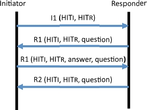
Figure 5.14. Base exchange procedure for HIP
Figure 5.15 illustrates the base exchange procedure, involving the DNS server. Before beginning the HIP base exchange, the initiator interrogates the DNS, using the responder’s DNS name, to obtain its HI and its IP address. After having received the necessary data, the initiator executes the basic exchange by means of four messages: I1, R1, I2 and R2.

Figure 5.15. HIP base exchange with DNS
5.7.2. SHIM6 (Level 3 Multihoming Shim Protocol for IPv6)
Like network-level multihoming protocols, SHIM6 also supports the separation of the identifying and localizing roles of the IP address. SHIM6 employs an intermediary SHIM sub-layer within the IP layer.
Unlike HIP, the SHIM6 approach does not introduce a new namespace for the identifiers. The terminal considers one of its IP addresses as its identifier. Known as the ULID (Upper-Layer Identifier), it is visible to the upper layers. Once the terminal’s ULID is chosen, it cannot be modified for the duration of the communication session. This mechanism ensures transparent operation of all upper-layer protocols in a multihoming environment, because these protocols always perceive a stable IPv6 address. The SHIM sub-layer handles the matching of the ULID and the terminal’s active address during the transmission.
As illustrated in Figure 5.16, terminal A has two addresses – IP1A and IP2A – and so does terminal B (IP1B, IP2B). The stable source and destination addresses perceived by the upper layers are, respectively, IP1A and IP1B. Suppose that the IP1A and IP1B address are no longer valid for the two terminals. If terminal A continues to send packets to terminal B, the application of terminal A indicates IP1A and IP1B as the packet’s source and destination addresses, because it is not aware of the change of addresses. When the SHIM sub-layer of terminal A receives that packet, it converts the indicated ULIDs into the real addresses of the two terminals. Then, the packet is sent over the address IP2A of terminal A to the address IP2B of terminal B. When the SHIM sub-layer of terminal B receives the packet, it translates the addresses back into ULIDs (IP1A for the source and IP1B for the destination) before sending data up to the next layer. Due to the matching between the ULID and the address performed by the SHIM sub-layer, the changes of address are totally transparent for the upper-layer protocols.

Figure 5.16. Example of matching in SHIM6
5.7.3. mCoA (Multiple Care-of-Addresses) in Mobile IPv6
MIP6 (Mobile IPv6) is the protocol used to manage mobility for IPv6. In the IP mobility architecture, each mobile node has a static HoA (Home Address) which is attributed by its home network. When the mobile node enters a host network, it obtains a new, temporary IP address known as the CoA (Care-of-Address). It informs its home agent (HA), which is in the home network. The HA stores, in its cache (Binding Cache), the match between the CoA and the HoA of the mobile node. Then, if there is any traffic destined for the HoA, it is intercepted by the HA and redirected to the mobile node’s true address using an IP tunnel. Consequently, the mobility of the mobile node becomes transparent to the corresponding nodes. The principle of Mobile IPv6 is illustrated in Figure 5.17.

Figure 5.17. Mobile IPv6
The limitations of Mobile IPv6 stem from the fact that the client can only register one CoA with his/her HA. Indeed, when the mobile node moves to a new network, it obtains a new CoA. The mobile node must inform its HA of this change in order for the HA to update its cache. The HA then replaces the old CoA with the new one. Consequently, at any given time, there can only be one association between a CoA and HoA.
With a view to being able to support multihoming, an extension to facilitate the registration of multiple CoAs was defined: a mobile node receiving several CoAs associated with its interfaces can register the same number of matches between its CoAs and its unique HoA with its HA. With this goal in mind, a binding identifier (BID) in the cache is used. Every instance of a registration (binding), which is equivalent to a match between a CoA and an HoA, is identified by a unique BID. By using one or more Binding Update messages, the mobile node informs its HA of its CoA/HoA matches and the corresponding BIDs. In its binding cache, the HA stores all the matches bound by the mobile node, as illustrated by Figure 5.18. Multipath transmission is managed by the mobile node. For outgoing data flows, the mobile node sends the traffic in accordance with its flow distribution algorithm. For incoming data flows, the mobile node defines the traffic preferences and informs the HA of those preferences. The HA then distributes the traffic destined for that mobile node via the different CoAs in keeping with the stated preferences.

Figure 5.18. Registration of several CoAs in Mobile IPv6
5.8. Transport-level multihoming
In the classic transport protocols TCP and UDP, each terminal uses a single address for a communication. If the terminal’s address changes, the connection is interrupted. With the evolution of access technology, it is quite common for a terminal to have several IP addresses associated with its interfaces. The solutions put forward for the transport level involve each terminal maintaining a list of IP addresses. One address can be replaced by another without the communication being broken. Transport-level multihoming protocols are extensions of TCP such as MPTCP (Multipath TCP), Multihomed TCP, TCP-MH, and SCTP (Stream Control Transmission Protocol). In this section, we shall discuss the two most widely used standardized protocols: SCTP and MPTCP.
5.8.1. SCTP (Stream Control Transmission Protocol)
Stream Control Transmission Protocol (SCTP) is a transport protocol which was defined by the IETF in 2000 and updated in 2007. Originally, this protocol was developed to transport voice signals on the IP network. As it is a transport protocol, SCTP is equivalent to other transport protocols such as TCP and UDP. SCTP offers better reliability, thanks to congestion-monitoring mechanisms, and the detection of duplicate packets and retransmission. In addition, it supports new services which set it apart from other transport protocols: multistreaming and multihoming. Unlike TCP, which is a byte-oriented protocol, SCTP is a message-oriented protocol. This is illustrated in Figure 5.19 – the data are sent and received in the form of messages.

Figure 5.19. SCTP architecture
When the SCTP transport service receives a data message from an application, it divides that message into chunks. There are two types of chunks: those containing user data and control chunks. In order to be sent to the lower layer, the chunks are encapsulated into SCTP packets. As Figure 5.20 indicates, an SCTP packet may contain several chunks of data or control chunks. Its size must be less than the MTU (Maximum Transmission Unit).

Figure 5.20. Structure of SCTP packet
The two SCTP terminals establish an SCTP connection. As mentioned above, SCTP can support multistreaming on a single connection. Unlike with TCP, several flows can be used simultaneously for communication in an SCTP connection. If congestion occurs on one of the paths, it only affects the flow being sent along that path, and has no impact on the other flows. Each SCTP flow independently numbers its chunks, using the sequence numbers StreamID and Stream Sequence Number (SSN).
Thanks to multistreaming, transport capacity is greatly improved. One of the most important services provided by SCTP is multihoming support. In this case, each SCTP terminal has a list of IP addresses linked to its interfaces.
When the connection is established, the SCTP terminals exchange their address lists. Of the IP addresses on that list, the terminal chooses one as a primary address, with the others being secondary addresses. In accordance with this principle, each SCTP connection has one primary path and multiple secondary paths. The primary path is used for data transmission. In case the primary path breaks down, SCTP uses one of those secondary paths to continue communication.
SCTP uses the Heartbeat mechanism to check whether a path is active. The Heartbeat message is periodically sent to each address advertised by the other terminal. The consecutive absence of an acknowledgement, Heartbeat-Ack, from the addressee indicates that a path is unavailable. Figure 5.21 illustrates the Heartbeat mechanism.
Terminal A periodically sends the Heartbeat message (every THB seconds) to check the availability of the path between two IP addresses (IP1a and IP1b). After n tests without acknowledgement, the path (IP1a, IP1b) is deemed to be inactive. If the primary path becomes inactive, a secondary path is used to send data until the primary path becomes active once more.
In each SCTP connection, a single path may be used for the data transmission, with the others being considered as backup paths. Multihoming stems from the possibility of using several paths simultaneously. Extensions of SCTP are needed in order for SCTP to be able to completely support multihoming.

Figure 5.21. Heartbeat mechanism
To support mobility, SCTP offers an extension called Mobile SCTP, which allows dynamic address reconfiguration. When a change of IP address takes place because the terminal has moved, that terminal sends an ASCONF (Address Configuration Change Chunk) message to request the addition of the new IP address, the deletion of the old address and possibly the changing of the primary address for that connection.
LS-SCTP (Load Sharing SCTP) is another extension of SCTP which allows the aggregation of bandwidth in SCTP. The terminals can simultaneously use several available paths for the transmission, ensuring the independence of the congestion control for each path.
The extension LS-SCTP is composed of two new elements:
- – a new parameter in the INIT and INIT-ACK chunks, which indicates whether the terminals support the extension;
- – two new types of chunks: an LS-Data (Load-Sharing Data) chunk, used for sending data, and an LS-SACK (Load-Sharing SACK) acknowledgement chunk, which provides selective acknowledgements on each path.
Figure 5.22 illustrates the architecture of LS-SCTP. On each side of the connection, we see an overall “Association Buffer”, a Path Assignment Module and a Path Monitor. LS-SCTP separates the flow control from the congestion control. The flow control is managed at the level of the connection. The terminals use the association buffer to receive data from all paths before sending them to the corresponding terminal or to the application.

Figure 5.22. Architecture of LS-SCTP
The fragmentation and reassembling of the data take place in the connection buffer. Congestion control is performed for each path. Each path has its own congestion control parameters, such as the size of the congestion window (cwnd), the slow-start threshold (ssthresh), the round-trip time (RTT), etc.
To separate the flow control from the congestion control, LS-STCP uses two different sequence numbers. The first is the ASN (Association Sequence Number), which is the sequence number for the active connection. It is used to order all the chunks received by the buffer on the connection to the receiver. The second is the sequence number of data chunks for each path, called the PSN (Path Sequence Number). It ensures that each path is reliable and controls the path congestion. In the LS-SCTP architecture, the Path Assignment module takes care of the distribution of the data between the available paths. This distribution is based on the availability of bandwidth. This module distributes chunks depending on the cwnd/RTT ratio of each path. Once the path is selected, the chunk provides a PID, indicating the path and a PSN.
Another difference between LS-SCTP and SCTP is the retransmission mechanism. To improve the likelihood of a retransmitted data chunk reaching the receiver, the retransmission uses a different path to that used for the previous attempted transmission. The Path Monitor module is responsible for overseeing the available paths and updating the list of active paths. This module updates the active path list when it obtains information from the network relating to the failure of an existing path or the availability of a new path. When the transmitter detects that a path is unavailable, it changes the status of that path to “inactive”. Inactive paths still remain associated with the connection. The transmitter continues to monitor them by means of the HeartBeat mechanism. As soon as an inactive path becomes active once more, Path Monitor adds it to the list of active paths and uses it for transmission.
5.8.2. CMT (Concurrent Multipath Transfer)
Multihoming is incompletely supported by SCTP. The only reason for having multiple paths available is to have redundancy in place. SCTP transmits via the primary path. The secondary paths are used only if the primary path fails. An extension of SCTP, called CMT (Concurrent Multipath Transfer), has been put forward for transmission via multiple paths.
In CMT, there is no distinction between the primary and secondary paths. All paths are equivalent, and are used simultaneously in data transmission. CMT employs the same system of sequencing numbers as SCTP. CMT uses the round-robin algorithm to send the data along the available paths. The sending of data to the transmitter is monitored by the size of the congestion window (CWND) for each path. CMT sends the data along a path as soon as the congestion window for that path becomes available. When several paths can be used for the transmission, the path is selected using the round-robin model. CMT fills the congestion window of each path before moving on to the next.
Despite the benefits of using multipath transmission, CMT brings with it the phenomenon of de-sequencing, which degrades performances, because of the fact that the paths in CMT may have different characteristics in terms of bandwidth and delay.
CMT identifies three causes of de-sequencing of data at the receiver’s end:
- – needless fast retransmissions. In a multipath transmission, paths may have different bandwidths and delays. It may be that an acknowledgement from a fast path will indicate the loss of a packet while that packet is still in transit on a slower path, and only arrives at its destination later on. CMT uses the same congestion control mechanism as TCP. When the transmitter receives three duplicate acknowledgements indicating the loss of a packet, it deems that packet to be lost in the network and triggers the fast retransmission of the packet. However, this retransmission is needless, because it is the de-sequencing which is the cause of the duplicated acknowledgements;
- – inaccurate updating of the congestion window. The mechanism by which the congestion window is updated only allows it to be increased if a new cumulative acknowledgement (CUM ACK) number is received by the transmitter. When the acknowledgements with the same CUM ACK have arrived, even if they contain new data gaps, the transmitter does not modify its congestion window. As the phenomenon of de-sequencing occurs regularly in CMT, several acknowledgements with the same acknowledgement are sent to the transmitter. When the data gaps are covered by a new acknowledgement, the congestion window is only increased with the new data acknowledged in the most recent acknowledgement. The previously-acknowledged data in the gaps do not contribute to the growth of the congestion window. In other words, the congestion window update does not exactly repeat the volume of data transmitted;
- – increased acknowledgement traffic. The principle of delayed acknowledgements in TCP is also used in SCTP. Instead of sending an acknowledgement for each and every packet received, the use of a group acknowledgement for several packets reduces acknowledgement traffic. SCTP uses this mechanism if the packets reach the receiver in the correct order. De-sequenced packets must be acknowledged immediately. However, as it is quite common for de-sequencing to occur in CMT, if the receiver cannot delay the sending of the acknowledgements, then acknowledgement traffic is greatly increased, which may impact the network’s performance. CMT includes the following solutions for these problems:
- - in order to prevent needless retransmissions, CMT offers the algorithm SFR (Split Fast Retransmit), which enables the transmitter to correctly interpret duplicate acknowledgements. SFR defines a virtual buffer for each destination within the transmitter’s retransmission buffer. With the additional information of each destination, such as the highest acknowledged TSN for each destination, the transmitter can distinguish between de-sequencing and actual data loss, with a view to correctly triggering fast retransmission. A chunk with the TSN T for destination M is deemed lost if and only if T is lower than the highest acknowledged TSN for destination M;
- - the algorithm CUC (Cwnd Update for CMT) is proposed to correctly update the congestion windows for the paths. At the level of the transmitter, each destination has a variable known as the PSEUDO-CUMACK, which represents the smallest anticipated TSN. Upon receipt of a SACK acknowledgement, the transmitter checks whether there is a change of PSEUDO-CUMACK for each destination. An increase of a PSEUDO-CUMACK triggers the updating of the congestion winder of the corresponding destination, even if the CUM ACK does not advance. Thus, the congestion window for each destination increases in parallel to the acknowledged data, without having to wait for the new CUM ACK;
- - CMT offers the algorithm DAC (Delayed ACK for CMT) to reduce acknowledgement traffic. DAC enables the CMT to delay the acknowledgement, even if the packets arrive out of sequence. As the sending of acknowledgements is often reported, the transmitter must closely analyze each acknowledgement received to detect any loss of data as quickly as possible. For this reason, in each acknowledgement, the receiver informs the transmitter of the number of data packets it has received since the sending of the least acknowledgement. This proposition requires modifications to be made to both transmitter and receiver.
5.8.3. MPTCP (Multipath TCP)
TCP is the most widely used transport protocol by Internet-based applications, but this protocol does not support multihoming. In spite of the existence of different paths, each TCP connection is limited to serving only one path for transmission. The simultaneous use of several paths for the same TCP session could improve data rate and offer better performances by strengthening the reliability of the connection. Multipath TCP, defined by the IETF, is a modified version of TCP which supports multihoming and allows the simultaneous transmission of data along several paths. As MPTCP is compatible with TCP, there is no need to modify existing applications to use its services. MPTCP is designed to gather together several independent TCP flows in a single MPTCP connection, ensuring transparency for the upper layers.
5.9. Conclusion
Mobile Cloud Networking is a paradigm which is growing enormously in importance, with the development of mobile terminals which are often not very powerful in comparison to the demand of certain applications. Mobile Cloud is another paradigm where clients come together to form a Cloud. As yet, this solution is not widely used, but it is likely to increase with the installation of more powerful boxes in vehicles.
Finally, we have examined network application controllers, which, along with SDN access points, are becoming increasingly common, and this solution represents the likely future of the discipline.