Chapter 13
Slightly More Complicated Testing
IN THIS CHAPTER
Working with two variables
Working with replications
Understanding interactions
Mixing variable-types
In Chapter 11, I show you how to test hypotheses with two samples. In Chapter 12, I show you how to test hypotheses when you have more than two samples. The common thread through both chapters is that one independent variable (also called a factor) is involved.
Many times, you have to test the effects of more than one factor. In this chapter, I show how to analyze two factors within the same set of data. Several types of situations are possible, and I describe Excel data analysis tools that deal with each one.
Cracking the Combinations
FarKlempt Robotics, Inc., manufactures battery-powered robots. They want to test three rechargeable batteries for these robots on a set of three tasks: climbing, walking, and assembling. Which combination of battery and task results in the longest battery life?
They test a sample of nine robots. They randomly assign each robot one battery and one type of task. FarKlempt tracks the number of days each robot works before recharging. The data are in Table 13-1.
TABLE 13-1 FarKlempt Robots: Number of Days before Recharging in Three Tasks with Three Batteries
Task |
Battery 1 |
Battery 2 |
Battery 3 |
Average |
|
Climbing |
12 |
15 |
20 |
15.67 |
|
Walking |
14 |
16 |
19 |
16.33 |
|
Assembling |
11 |
14 |
18 |
14.33 |
|
Average |
12.33 |
15.00 |
19.00 |
15.44 |
This calls for two hypothesis tests:
H0: μBattery1 = μBattery2 = μBattery3
H1: Not H0
and
H0: μClimbing = μWalking = μAssembling
H1: Not H0
In both tests, set α = .05.
Breaking down the variances
The appropriate analysis for these tests is an analysis of variance (ANOVA). Each variable — Batteries and Tasks — is also called a factor. So this analysis is called a two-factor ANOVA.
To understand this ANOVA, consider the variances inside the data. First, focus on the variance in the whole set of nine numbers — MST. (T in the subscript stands for Total.) The mean of those numbers is 15.44. Because it’s the mean of all the numbers, it goes by the name grand mean.
This variance is
The means of the three batteries (the column means) also vary from 15.44. That variance is
Why does the 3 appear as a multiplier of each squared deviation? When you deal with means, you have to take into account the number of scores that produce each mean.
Similarly, the means of the tasks (the row means) vary from 15.44:
One variance is left. It’s called MSError. This is what remains when you subtract the SSBatteries and the SSTasks from the SST, and divide that by the df that remains when you subtract dfBatteries and dfTasks from dfT:
To test the hypotheses, you calculate one F for the effects of the batteries and another for the effects of the tasks. For both, the denominator (the error term) is MSError:

Each F has 2 and 4 degrees of freedom. With α = .05, the critical F in each case is 6.94. The decision is to reject H0 for the batteries (they differ from one another to an extent greater than chance), but not for the tasks.
To zero in on the differences for the batteries, you carry out planned comparisons among the column means. (See Chapter 12 for the details.)
Data analysis tool: Anova: Two-Factor Without Replication
Excel’s Anova: Two-Factor Without Replication tool carries out the analysis I just outlined. (I use this tool for another type of analysis in Chapter 12.) Without Replication means that only one robot is assigned to each battery-task combination. If you assign more than one to each combination, that’s replication.
Figure 13-1 shows this tool’s dialog box along with the data for the Batteries-Tasks example.

FIGURE 13-1: The Anova: Two-Factor Without Replication data analysis tool dialog box along with the Batteries-Tasks data.
The steps for using this tool are:
-
Enter the data into the worksheet, and include labels for the rows and columns.
For this example, the labels for the tasks are in cells B4, B5, and B6. The labels for the batteries are in cells C3, D3, and E3. The data are in cells C4 through E6.
- Select DATA | Data Analysis to open the Data Analysis dialog box.
- In the Data Analysis dialog box, scroll down the Analysis Tools list and select Anova: Two-Factor Without Replication.
-
Click OK to open the Anova: Two-Factor Without Replication dialog box.
This is the dialog box in Figure 13-1.
-
In the Input Range box, enter the cell range that holds all the data.
For the example, the data range is $B$3:$E$6. Note the $ signs for absolute referencing. Note also — and this is important — the row labels are part of the data range. The column labels are, too. The first cell in the data range, B2, is blank, but that’s okay.
-
If the cell ranges include column headings, select the Labels option.
I included the headings in the ranges, so I selected the box.
- The Alpha box has 0.05 as a default. Change that value if you want a different α.
-
In the Output Options, select a radio button to indicate where you want the results.
I selected New Worksheet Ply to put the results on a new page in the worksheet.
-
Click OK.
Because I selected New Worksheet Ply, a newly created page opens with the results.
Figure 13-2 shows the tool’s output, after I expanded the columns. The output features two tables: SUMMARY and ANOVA.

FIGURE 13-2: Output from the Anova: Two-Factor Without Replication data analysis tool.
The SUMMARY table is in two parts. The first part provides summary statistics for the rows. The second part provides summary statistics for the columns. Summary statistics include the number of scores in each row and in each column along with the sums, means, and variances.
The ANOVA table presents the Sums of Squares, df, Mean Squares, F, P-values, and critical F for the indicated df. The table features two values for F. One F is for the rows, and the other is for the columns. The P-value is the proportion of area that the F cuts off in the upper tail of the F-distribution. If this value is less than .05, reject H0.
In this example, the decisions are to reject H0 for the batteries (the columns) and to not reject H0 for the tasks (the rows).
Cracking the Combinations Again
The preceding analysis involves one score for each combination of the two factors. Assigning one individual to each combination is appropriate for robots and other manufactured objects, where you can assume that one object is pretty much the same as another.
When people are involved, it’s a different story. Individual variation among humans is something you can’t overlook. For this reason, it’s necessary to assign a sample of people to a combination of factors — not just one person.
Rows and columns
I illustrate with an example. Imagine that a company has two methods of presenting its training information. One is via a person who presents the information orally, and the other is via a text. Imagine also that the information is presented in either a humorous way or in a technical way. I refer to the first factor as Presentation Method and to the second as Presentation Style.
Combining the two levels of Presentation Method with the two levels of Presentation Style gives four combinations. The company randomly assigns 4 people to each combination, for a total of 16 people. After providing the training, they test the 16 people on their comprehension of the material.
Figure 13-3 shows the combinations, the four comprehension scores within each combination, and summary statistics for the combinations, rows, and columns.

FIGURE 13-3: Combining the levels of Presentation Method with the levels of Presentation Style.
Here are the hypotheses:
H0: μSpoken = μText
H1: Not H0
and
H0: μHumorous = μTechnical
H1: Not H0
Because the two presentation methods (Spoken and Text) are in the rows, I refer to Presentation Type as the row factor. The two presentation styles (Humorous and Technical) are in the columns, so Presentation Style is the column factor.
Interactions
When you have rows and columns of data, and you’re testing hypotheses about the row factor and the column factor, you have an additional consideration. Namely, you have to be concerned about the row-column combinations. Do the combinations result in peculiar effects?
For the example I present, it’s possible that combining Spoken and Text with Humorous and Technical yields something unexpected. In fact, you can see that in the data in Figure 13-3: For Spoken presentation, the Humorous style produces a higher average than the Technical style. For Text presentation, the Humorous style produces a lower average than the Technical style.
 A situation like that is called an interaction. In formal terms, an interaction occurs when the levels of one factor affect the levels of the other factor differently. The label for the interaction is row factor X column factor, so for this example, that’s Method X Type.
The hypotheses for this are
H0: Presentation Method does not interact with Presentation Style
H1: Not H0
The analysis
The statistical analysis, once again, is an analysis of variance (ANOVA). As is the case with the earlier ANOVAs I show you, it depends on the variances in the data.
The first variance is the total variance, labeled MST. That’s the variance of all 16 scores around their mean (the “grand mean”), which is 44.81:
The denominator tells you that df = 15 for MST.
The next variance comes from the row factor. That’s MSMethod, and it’s the variance of the row means around the grand mean:
The 8 multiplies each squared deviation because you have to take into account the number of scores that produced each row mean. The df for MSMethod is the number of rows – 1, which is 1.
Similarly, the variance for the column factor is
The df for MSStyle is 1 (the number of columns – 1).
Another variance is the pooled estimate based on the variances within the four row-column combinations. It’s called the MSWithin, or MSW. (For details on MSw and pooled estimates, see Chapter 12.). For this example,
This one is the error term (the denominator) for each F that you calculate. Its denominator tells you that df = 12 for this MS.
The last variance comes from the interaction between the row factor and the column factor. In this example, it’s labeled MSMethod X Type. You can calculate this in a couple of ways. The easiest way is to take advantage of this general relationship:
And this one:
Another way to calculate this is
The MS is
For this example,
To test the hypotheses, you calculate three Fs:

For df = 1 and 12, the critical F at α = .05 is 4.75. (You can use the Excel function FINV to verify.) The decision is to reject H0 for the Presentation Method and for the Method X Style interaction, and to not reject H0 for the Presentation Style.
Data analysis tool: Anova: Two-Factor With Replication
Excel provides a data analysis tool that handles everything I just spelled out in the previous section. This one is called Anova: Two-Factor With Replication. Replication means that you have more than one score in each row-column combination.
Figure 13-4 shows this tool’s dialog box along with the data for the batteries-tasks example.

FIGURE 13-4: The Anova: Two-Factor With Replication data analysis tool dialog box along with the type-method data.
The steps for using this tool are:
-
Enter the data into the worksheet and include labels for the rows and columns.
For this example, the labels for the presentation methods are in cells B3 and B7. The presentation types are in cells C2 and D2. The data are in cells C3 through D10.
- Select Data | Data Analysis to open the Data Analysis dialog box.
- In the Data Analysis dialog box, scroll down the Analysis Tools list and select Anova: Two-Factor With Replication.
-
Click OK to open the Anova: Two-Factor With Replication dialog box.
This is the dialog box in Figure 13-4.
-
In the Input Range box, type the cell range that holds all the data.
For the example, the data are in $B$2:$D$10. Note the $ signs for absolute referencing. Note also — again, this is important — the labels for the row factor (presentation method) are part of the data range. The labels for the column factor are part of the range, too. The first cell in the range, B2, is blank, but that’s okay.
-
In the Rows per Sample box, type the number of scores in each combination of the two factors.
I typed 4 into this box.
- The Alpha box has 0.05 as a default. Change that value if you want a different α.
-
In the Output Options, select a radio button to indicate where you want the results.
I selected New Worksheet Ply to put the results on a new page in the worksheet.
-
Click OK.
Because I selected New Worksheet Ply, a newly created page opens with the results.
Figure 13-5 shows the tool’s output, after I expand the columns. The output features two tables: SUMMARY and ANOVA.

FIGURE 13-5: Output from the Anova: Two-Factor With Replication data analysis tool.
The SUMMARY table is in two parts. The first part provides summary statistics for the factor combinations and for the row factor. The second part provides summary statistics for the column factor. Summary statistics include the number of scores in each row-column combination, in each row, and in each column along with the counts, sums, means, and variances.
The ANOVA table presents the Sums of Squares, df, Mean Squares, F, P-values, and critical F for the indicated df. The table features three values for F. One F is for the row factor, one for the column factor, and one for the interaction. In the table, the row factor is called Sample. The P-value is the proportion of area that the F cuts off in the upper tail of the F-distribution. If this value is less than .05, reject H0.
In this example, the decisions are to reject H0 for the Presentation Method (the row factor, labeled Sample in the table), to not reject H0 for the Presentation Style (the column factor), and to reject H0 for the interaction.
Two Kinds of Variables … at Once
What happens when you have a Between Groups variable and a Within Groups variable … at the same time? (It’s called a Mixed design.) How can that happen?
Very easily. Here’s an example. Suppose you want to study the effects of presentation media on the reading speeds of fourth-graders. You randomly assign your fourth-graders (I’ll call them subjects) to read either e-readers or books. That’s the Between Groups variable.
Let’s say you’re also interested in the effects of font. So you assign each subject to read each of these fonts: Haettenschweiler, Arial, and Calibri. (I’ve never seen a document in Haettenschweiler, but it’s my favorite font because “Haettenschweiler” is fun to say. Try it. Am I right?) Because each subject reads all the fonts, that’s the Within Groups variable. For completeness, you have to randomly order the fonts for each subject.
What would the ANOVA table look like? Table 13-2 shows you in a generic way. It’s categorized into a set of sources that make up Between Groups variability, and a set of sources that make up Within Groups variability.
TABLE 13-2 The ANOVA Table for the Mixed ANOVA (One Between Groups Variable and One Within Groups Variable)
Source |
SS |
df |
MS |
F |
|
Between |
SSBetween |
dfBetween | ||
|
A |
SSA |
dfA |
SSA/dfA |
MSA/MSS/A |
|
S/A |
SSS/A |
dfS/A |
SSS/A/dfS/A |
|
|
Within |
SSWithin |
dfWithin | ||
|
B |
SSB |
dfB |
SSB/dfB |
MSB/MSB X S/A |
|
A X B |
SSA X B |
dfA X B |
SSA X B /dfA X B |
MSA X B/MSB X S/A |
|
B X S/A |
SSB X S/A |
dfB XS/A |
SSB X S/A/dfB X S/A |
|
|
Total |
SSTotal |
dfTotal | ||
In the Between category, A is the name of the Between Groups variable. Read “S/A” as “S within A.” This just says that the people in one level of A are different from the people in the other levels of A.
In the Within category, B is the name of the Within Groups. A X B is the interaction of the two variables. B X S/A is something like the B variable interacting with subjects within A. As you can see, anything associated with B falls into the Within Groups category.
The first thing to note is the three F-ratios. The first one tests for differences among the levels of A, the second for differences among the levels of B, and the third for the interaction of the two. Notice also that the denominator for the first F-ratio is different from the denominator for the other two. This happens more and more as ANOVAs increase in complexity.
Next, it’s important to be aware of some relationships. At the top level:
SSBetween + SSWithin = SSTotal
dfBetween + dfWithin = dfTotal
The Between component breaks down further:
SSA + SSS/A = SSBetween
dfA + dfS/A = dfBetween
The Within component breaks down, too:
SSB + SSA X B + SSB X S/A = SSWithin
dfB + dfA X B + dfB X S/A = dfWithin
Knowing these relationships helps complete the ANOVA table after Excel has gone through its paces.
Using Excel with a Mixed Design
Someday, Excel’s Analysis ToolPak might have a choice labeled ANOVA: Mixed Design. That day, unfortunately, is not today. Instead, I use two ToolPak tools and knowledge about this type of design to provide the analysis.
I begin with the data for the study I describe earlier. Figure 13-6 shows a worksheet with the data. The levels of the Between Group variable, Media (the A variable), are in the left column. The levels of the Within Group variable, Font (the B variable), are in the top row. Each cell entry is a reading speed in words per minute.

FIGURE 13-6: Data for a study with a Between Group variable and a Within Group variable.
Next, Figure 13-7 shows the completed ANOVA table.

FIGURE 13-7: The completed ANOVA table for the analysis of the data in Figure 13-6.
How do you get there? Surprisingly, it’s pretty easy, although quite a few steps are involved. All you have to do is run two ANOVAs on the same data and combine the ANOVA tables. The relationships I show you in the preceding section complete the pieces in the puzzle.
Follow these steps:
-
With the data entered into a worksheet, select Data | Data Analysis.
This opens the Data Analysis dialog box.
-
From the Data Analysis dialog box, select Anova: Two-Factor Without Replication.
This opens the Anova: Two-Factor Without Replication dialog box.
-
In the Input Range box, enter the cell range that holds the data.
For this example, that’s C1:F9. This range includes the column headers, so select the Labels check box.
-
With the New Worksheet Ply radio button selected, click OK.
The result is the ANOVA table in Figure 13-8.
-
Modify the ANOVA table: Insert rows for terms from the second ANOVA, change names of the Sources of Variance, and delete unnecessary values.
First, insert four rows between Rows and Columns (between Row 20 and the original Row 21).
Next, change Rows to Between Group and Columns to Font (the name of the B variable).
Then, delete all the information from the row that has Error in the Source column.
Finally, delete the F-ratios, P-values, and F-crits. The ANOVA table now looks like Figure 13-9.
- Once again, select Data | Data Analysis.
- This time, from the Data Analysis dialog box choose ANOVA: Two-Factor With Replication.
-
In the Input Range box, enter the cell array that holds the data, including the column headers.
To do this, select C1:F9 in the worksheet.
-
In the Rows Per Sample box, enter the number of subjects within each level of the Between Groups variable.
For this example, that’s 4.
- With the New Worksheet Ply radio button selected, click OK.
-
Copy the resulting ANOVA table and paste it into the worksheet with the first ANOVA, just below the first ANOVA table.
The worksheet should look like Figure 13-10.
-
Add Within Group to the first ANOVA table, four rows under Between Group, and calculate values for SS and df.
Type Within Group into row 24. The SS for Within Group is the SS Total – SS Between Group (B28-B20). The df for Within Group is the df Total – df Between Group (C28-C20).
-
Copy the Sample row of data from the second ANOVA table and paste it into the first ANOVA table just below Between Group.
Copy and paste just the Source name (Sample), its SS and its df.
-
Change Sample to the name of the Between Group variable (the A variable).
Change Sample to Media.
-
In the next row, enter the name of the source for S/A, and calculate its SS, df, and MS.
Enter Subject/Media. The SS is the SS Between Group – SS Media (B20:B21). The df is the df Between Group – df Media (C20:C21). The MS is the SS divided by the df (B22/C22).
-
In the appropriate cell, calculate the F ratio for the A variable.
That’s MS Media divided by MS Subject/Media (D21/D22) calculated in E21. The ANOVA table now looks like Figure 13-11.
-
From the second ANOVA table, copy the Interaction, its SS, its df, and its MS, and paste into the first ANOVA table in the row just below the name of the B variable. Change Interaction to the name of the interaction between the A variable and the B variable.
Copy the information from Row 34 into Row 26, just below Font. Change Interaction to Media X Font.
-
In the next row, type the name of the source for B X S/A and calculate its SS, df, and MS.
Type Font X Subject/Media into A27. The SS is the SS Within Group – SS Font – SS Media X Font (B24 – B25 – B26). The df is the df Within Group – df Font – df Media X Font (C24 – C25 – C26). The MS is the SS divided by the df (B27/C27).
-
In the appropriate cells, calculate the remaining F-ratios.
In E25, divide D25 by D27. In E26, divide D26 by D27. For clarity, insert a row just above Total. The table now looks like Figure 13-12.

FIGURE 13-8: The ANOVA table for the first of two ANOVAs.

FIGURE 13-9: The first ANOVA table after modifications.

FIGURE 13-10: The modified first ANOVA table and the second ANOVA table.
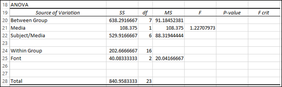
FIGURE 13-11: The ANOVA table with the information for the Between Group variable and part of the information for the Within Group variable.

FIGURE 13-12: The ANOVA table with all the SS, df, MS and F-ratios.
To make the table look like Figure 13-7, shown earlier, use F.DIST.RT to find the P-values, and F.INV.RT to find the F-crits. (I discuss these functions in Chapter 11.) You can also delete the value for MSBetween Group, because it serves no purpose.
For some nice cosmetic effects, indent the sources under the main categories (Between Groups and Within Groups), and center the df for the main categories.
And what about the analysis? The completed ANOVA table shows no effect of Media, a significant effect of Font, and a Media X Font interaction.
This procedure uses Anova: Two-Factor With Replication, a tool that depends on an equal number of replications (rows) for each combination of factors. So for this procedure to work, you have to have an equal number of people in each level of the Between Groups variable.
Graphing the Results
Because this isn’t a built-in tool, Excel doesn’t produce the descriptive statistics for each combination of conditions. You have to have those statistics (means and standard errors) to create a chart of the results.
This, of course, isn’t hard to do. Figure 13-13 shows the table of means and the table of standard errors along with the data. Each entry in the means table is just the AVERAGE function applied to the appropriate cell range. So the value in D13 is
=AVERAGE(D2:D5)

FIGURE 13-13: The data along with the Means table and the Standard Errors table.
Each entry in the Standard Errors table is the result of applying three functions to the appropriate cell range. To show you an example, I’ve selected D18 so that its value appears in the Formula bar in the figure:
=STDEV.S(D2:D5)/SQRT(COUNT(D2:D5))
Figure 13-14 shows the column chart for the results. To create it, I select the means table (C12:F14) and select Insert | Recommended Charts and then select the Clustered Column option. Then I added the error bars for the standard errors (see Chapter 22) and tweaked the chart. (Refer to Chapter 3.)

FIGURE 13-14: Graphing the results.
The chart clearly illustrates the Media X Font interaction. For Haettenschweiler, the reading speed is higher with the book. For each of the others, the reading speed is higher with the E-reader.
After the ANOVA
As I point out in Chapter 12, a significant result in an ANOVA tells you that an effect is lurking somewhere in the data. Post-analysis tests tell you where. Two types of tests are possible — either planned or unplanned. Chapter 12 provides the details.
In this example, the Between Groups variable has only two levels. For this reason, had a significant effect resulted, no further test would be necessary. The Within Groups variable, Font, is significant. Ordinarily, the test would proceed as in Chapter 12. In this case, however, the interaction between Media and Font necessitates a different path.
With the interaction, post-analysis tests can proceed in either (or both) of two ways. You can examine the effects of each level of the A variable on the levels of the B variable, or you can examine the effects of each level of the B variable on the levels of the A variable. Statisticians refer to these as simple main effects.
For this example, the first way examines the means for the three fonts in a book and the means for the three fonts in the E-reader. The second way examines the means for the book versus the mean for the E-reader with Haettenschweiler font, with Arial, and with Calibri.
Statistics texts provide complicated formulas for calculating these analyses. Excel makes them easy. To analyze the three fonts in the book, do a repeated measures ANOVA for Subjects 1 through 4. To analyze the three fonts in the E-reader, do a repeated measures ANOVA for Subjects 5 through 8.
For the analysis of the book versus the E-reader in the Haettenschweiler font, that’s a single-factor ANOVA for the Haettenschweiler data. To do this, you’d have to rearrange the numbers into two columns. Of course, you’d go through a similar procedure for each of the other fonts.