
Markov Chain Monte Carlo Methods
9.1 Introduction
Markov Chain Monte Carlo (MCMC) methods encompass a general framework of methods introduced by Metropolis et al. [197] and Hastings [138] for Monte Carlo integration. Recall (see Section 5.2) that Monte Carlo integration estimates the integral
∫Ag(t)dt
with a sample mean, by restating the integration problem as an expectation with respect to some density function f(·). The integration problem then is reduced to finding a way to generate samples from the target density f(·).
The MCMC approach to sampling from f(·) is to construct a Markov chain with stationary distribution f(·), and run the chain for a sufficiently long time until the chain converges (approximately) to its stationary distribution.
This chapter is a brief introduction to MCMC methods, with the goal of understanding the main ideas and how to implement some of the methods in R. In the following sections, methods of constructing the Markov chains are illustrated, such as the Metropolis and Metropolis-Hastings algorithms, and the Gibbs sampler, with applications. Methods of checking for convergence are briefly discussed. In addition to references listed in Section 5.1, see e.g. Casella and George [40], Chen, Shao, and Ibrahim [44], Chib and Greenberg [47], Gamerman [103], Gelman et al. [108], or Tierney [272]. For a thorough, accessible treatment with applications, see Gilks, Richardson, and Spiegelhalter [120]. For reference on Monte Carlo methods including extensive treatment of MCMC methods see Robert and Casella [228].
9.1.1 Integration problems in Bayesian inference
Many applications of Markov Chain Monte Carlo methods are problems that arise in Bayesian inference. From a Bayesian perspective, in a statistical model both the observables and the parameters are random. Given observed data x = {x1, ... , xn}, and parameters θ, x depends on the prior distribution fθ(θ). This dependence is expressed by the likelihood f(x1,...,xn|θ). The joint distribution of (x, θ) is therefore
fx,θ(x,θ)=fx|θ(x1,...,xn|θ)fθ(θ).
One can then update the distribution of θ conditional on the information in the sample x = {x1, ... , xn}, so that by Bayes Theorem the posterior distribution of θ is given by
fθ|x(θ|x)=fx|θ(x1,...,xn|θ)fθ(θ)∫fx|θ(x1,...,xn|θ)fθ(θ)dθ=fx|θ(x)fθ(θ)∫fx|θ(x)fθ(θ)dθ.
Then the conditional expectation of a function g(θ) with respect to the posterior density is
E[g(θ|x)]=∫g(θ)fθ|x(θ)dθ=∫g(θ)fx|θ(x)fθ(θ)dθ∫fx|θ(x)fθ(θ)dθ.(9.1)
To state the problem in more general terms,
E[g(Y)]=∫ g(t)π(t)dt∫ π(t)dt,(9.2)
where π(·) is (proportional to) a density or a likelihood. If π(·) is a density function, then (9.2) is just the usual definition E[g(Y)]=∫g(t)fY(t)dt If π(·) is a likelihood, then the normalizing constant in the denominator is needed. In Bayesian analysis, π(·) is a posterior density. The expectation (9.2) can be evaluated even if π(·) is known only up to a constant. This simplifies the problem because in practice the normalizing constant for a posterior density fθ|x(θ)is often difficult to evaluate.
The practical problem, however, is that the integrations in (9.2) are often mathematically intractable, and difficult to compute by numerical methods, especially in higher dimensions. Markov Chain Monte Carlo provides a method for this type of integration problem.
9.1.2 Markov Chain Monte Carlo Integration
The Monte Carlo estimate of E[g(θ)]=∫g(θ)fθ|x(θ)dθis the sample mean
ˉg=1mm∑i=1g(xi),
where x1, ... , xm is a sample from the distribution with density fθ|x. If x1, ... , xm are independent (it is a random sample) then by the laws of large numbers, the sample mean ˉg converges in probability to E[g(θ)] as sample size n tends to infinity. In this case, one can in principle draw as large a Monte Carlo sample as required to obtain the desired precision in the estimate ˉg. Here the first “MC” in “MCMC” is not needed; Monte Carlo integration can be used.
However, in a problem such as (9.1) it may be quite difficult to implement a method for generating independent observations from the density fθ|x. Nevertheless, even if the sample observations are dependent, a Monte Carlo integration can be applied if the observations can be generated so that their joint density is roughly the same as the joint density of a random sample. This is where the first “MC” comes to the rescue. Markov Chain Monte Carlo methods estimate the integral in (9.1) or (9.2) by Monte Carlo integration, and the Markov Chain provides the sampler that generates the random observations from the target distribution.
By a generalization of the strong law of large numbers, if {X0,X1,X2,...} is a realization of an irreducible, ergodic Markov Chain with stationary distribution π, then
¯g(X)m=1mm∑t=0g(Xt)
converges with probability one to E[g(X)] as m → ∞, where X has the stationary distribution π and the expectation is taken with respect to π (provided the expectation exists).
For a brief review of discrete-time discrete-state-space Markov Chains see Section 2.8. For an introduction to Markov chains and stochastic processes see Ross [234].
9.2 The Metropolis-Hastings Algorithm
The Metropolis-Hastings algorithms are a class of Markov Chain Monte Carlo methods including the special cases of the Metropolis sampler, the Gibbs sampler, the independence sampler, and the random walk. The main idea is to generate a Markov Chain {Xt|t=0,1,2,... }such that its stationary distribution is the target distribution. The algorithm must specify, for a given state Xt, how to generate the next state Xt+1. In all of the Metropolis-Hastings (M-H) sampling algorithms, there is a candidate point Y generated from a proposal distribution g(⋅|Xt). If this candidate point is accepted, the chain moves to state Y at time t + 1 and Xt+1 = Y ; otherwise the chain stays in state Xt and Xt+1 = Xt. Note that the proposal distribution can depend on the previous state Xt. For example, if the proposal distribution is normal, one choice for g(⋅|Xt)might be Normal(μt = Xt, σ2) for some fixed σ2.
The choice of proposal distribution is very flexible, but the chain generated by this choice must satisfy certain regularity conditions. The proposal distribution must be chosen so that the generated chain will converge to a stationary distribution – the target distribution f. Required conditions for the generated chain are irreducibility, positive recurrence, and aperiodicity (see [229]). A proposal distribution with the same support set as the target distribution will usually satisfy these regularity conditions. Refer to [121, Ch. 7-8], [228, Ch. 7] or [229] for further details on the choice of proposal distribution.
9.2.1 Metropolis-Hastings Sampler
The Metropolis-Hastings sampler generates the Markov chain {X0, X1,... } as follows.
- Choose a proposal distribution g(⋅|Xt)(subject to regularity conditions stated above).
- Generate X0 from a distribution g.
- Repeat (until the chain has converged to a stationary distribution according to some criterion):
- Generate Y from g(⋅|Xt).
- Generate U from Uniform(0,1).
- If
U≤f(Y)g(Xt|Y)f(Xt)g(Y|Xt)
accept Y and set Xt+1 = Y ; otherwise set Xt+1 = Xt.
- Increment t.
Observe that in step (3c) the candidate point Y is accepted with probability
α(Xt,Y)=min(1,f(Y)g(Xt|Y)f(Xt)g(Y|Xt)),(9.3)
so that it is only necessary to know the density of the target distribution f up to a constant.
Assuming that the proposal distribution satisfies the regularity conditions, the Metropolis-Hastings chain will converge to a unique stationary distribution π. The algorithm is designed so that the stationary distribution of the Metropolis-Hastings chain is indeed the target distribution, f.
Suppose (r,s) are two elements of the state space of the chain, and without loss of generality suppose that f(s)g(r|s)≥f(r)g(s|r). Thus, α(r,s) = 1 and the joint density of (Xt, Xt+1) at (r,s) is f(r)g(s|r). The joint density of (Xt, Xt+1) at (s,r) is
f(s)g(r|s)α(s,r)=f(s)g(r|s)(f(r)g(s|r)f(s)g(r|s))=f(r)g(s|r).
The transition kernel is
k(r,s)=α(r,s)g(s|r)+I(s=r)[1−∫α(r,s)g(s|r)ds].
(The second term in K(r, s) arises when the candidate point is rejected and Xt+1 = Xt.) Hence we have the system of equations
α(r,s)f(r)g(s|r)=α(s,r)f(s)g(r|s),I(s=r)[1−∫α(r,s)g(s|r)ds]f(r)]=I(r=s)[1−∫α(s,r)g(r|s)ds]f(s)]
for the Metropolis-Hastings chain, and f satisfies the detailed balance condition K(s,r)f(s) = K(r,s)f(r). Therefore f is the stationary distribution of the chain. See Theorems 6.46 and 7.2 in [228].
Example 9.1 (Metropolis-Hastings sampler)
Use the Metropolis-Hastings sampler to generate a sample from a Rayleigh distribution. The Rayleigh density [156, (18.76)] is
f(x)=xσ2e−x2/(2σ2), x≥0,σ>0.
The Rayleigh distribution is used to model lifetimes subject to rapid aging, because the hazard rate is linearly increasing. The mode of the distribution is at σ,E[X]=σ√π/2and Var(X)=σ2(4−π)/2.
For the proposal distribution, try the chisquared distribution with degrees of freedom Xt. Implementation of a Metropolis-Hastings sampler for this example is as follows. Note that the base of the array in R is 1, so we initialize the chain at X0 in x[1].
- Set g(⋅|X)to the density of χ2(X).
- Generate X0 from distribution χ2(1) and store in x[1].
- Repeat for i = 2, ... , N:
- Generate Y from χ2(df = Xt) = χ2(df=x[i-1]).
- Generate U from Uniform(0, 1).
- With Xt = x[i-1], compute
r(Xt,Y)=f(Y)g(Xt|Y)f(Xt)g(Y|Xt),
where f is the Rayleigh density with parameter σ,g(Y|Xt)is the χ2(df = Xt) density evaluated at Y , and g(Xt|Y)is the χ2(df = Y) density evaluated at Xt.
If U ≤ r(Xt, Y) accept Y and set Xt+1 = Y ; otherwise set Xt+1 = Xt. Store Xt+1 in x[i].
- Increment t.
The constants in the densities cancel, so
r(xt,y)=f(y)g(xt|y)f(xt)g(y|xt)=ye−y2/2σ2xte−x2t/2σ2×|Γ(xt2)2xt/2xy/2−1te−xt/2Γ(y2)2y/2yxt/2−1e−y/2.
This ratio can be simplified further, but in the following simulation for clarity we will evaluate the Rayleigh and chisquare densities separately. The following function evaluates the Rayleigh(σ) density.
f <- function(x, sigma) {
if (any(x < 0)) return (0)
stopifnot(sigma > 0)
return((x / sigma^2) * exp(-x^2 / (2*sigma^2)))
}
In the simulation below, a Rayleigh(σ = 4) sample is generated using the chisquare proposal distribution. At each transition, the candidate point Y is generated from χ2(ν = Xi−1)
xt <- x[i-1]
y <- rchisq(1, df = xt)
and for each y, the numerator and denominator of r(Xi−1,Y) are computed in num and den. The counter k records the number of rejected candidate points.
m <- 10000
sigma <- 4
x <- numeric(m)
x[1] <- rchisq(1, df=1)
k <- 0
u <- runif(m)
for (i in 2:m) {
xt <- x[i-1]
y <- rchisq(1, df = xt)
num <- f(y, sigma) * dchisq(xt, df = y)
den <- f(xt, sigma) * dchisq(y, df = xt)
if (u[i] <= num/den) x[i] <- y else {
x[i] <- xt
k <- k+1 #y is rejected
}
}
> print(k)
[1] 4009
In this example, approximately 40% of the candidate points are rejected, so the chain is somewhat inefficient.
To see the generated sample as a realization of a stochastic process, we can plot the sample vs the time index. The following code will display a partial plot starting at time index 5000.
index <- 5000:5500
y1 <- x[index]
plot(index, y1, type="l", main="", ylab="x")
The plot is shown in Figure 9.1. Note that at times the candidate point is rejected and the chain does not move at these time points; this corresponds to the short horizontal paths in the graph.

Part of a chain generated by a Metropolis-Hastings sampler of a Rayleigh distribution in Example 9.1.
Example 9.1 is a simple example intended to illustrate how to implement a Metropolis-Hastings sampler. There are better ways to generate samples from Rayleigh distributions. In fact, an explicit formula for the quantiles of the Rayleigh distribution are given by
xq=F−1(q)=σ{−2log(1−q)}1/2, 0<q<1.(9.4)
Using F−1 one could write a simple generator for Rayleigh using the inverse transform method of Section 3.2.1 with antithetic sampling (Section 5.4).
Example 9.2 (Example 9.1, cont.)
The following code compares the quantiles of the target Rayleigh(σ = 4) distribution with the quantiles of the generated chain in a quantile-quantile plot (QQ plot).
b <- 2001 #discard the burnin sample
y <- x[b:m]
a <- ppoints(100)
QR <- sigma * sqrt(-2 * log(1 - a)) #quantiles of Rayleigh
Q <- quantile(x, a)
qqplot(QR, Q, main="",
xlab="Rayleigh Quantiles", ylab="Sample Quantiles")
hist(y, breaks="scott", main="", xlab="", freq=FALSE)
lines(QR, f(QR, 4))
The histogram of the generated sample with the Rayleigh(σ = 4) density superimposed is shown in Figure 9.2(a) and the QQ plot is shown in Figure 9.2(b). The QQ plot is an informal approach to assessing the goodness-of-fit of the generated sample with the target distribution. From the plot, it appears that the sample quantiles are in approximate agreement with the theoretical quantiles.

Histogram with target Rayleigh density and QQ plot for a Metropolis-Hastings chain in Example 9.1.
9.2.2 The Metropolis Sampler
The Metropolis-Hastings sampler [138, 197] is a generalization of the Metropolis sampler [197]. In the Metropolis algorithm, the proposal distribution is symmetric. That is, the proposal distribution g(⋅|Xt)satisfies
g(X|Y)=g(Y|X),
so that in (9.3) the proposal distribution g cancels from
r(Xt,Y)=f(Y)g(Xt|Y)f(Xt)g(Y|Xt),
and the candidate point Y is accepted with probability
α(Xt,Y)=min(1,f(Y)f(Xt)).
9.2.3 Random Walk Metropolis
The random walk Metropolis sampler is an example of a Metropolis sampler. Suppose the candidate point Y is generated from a symmetric proposal distribution g(Y|Xt)=g(|Xt−Y|). Then at each iteration, a random increment Z is generated from g(·), and Y is defined by Y = Xt+Z. For example, the random increment might be normal with zero mean, so that the candidate point is Y|Xt~Normal(Xt,σ2)for some fixed σ2 > 0.
Convergence of the random walk Metropolis is often sensitive to the choice of scale parameter. When variance of the increment is too large, most of the candidate points are rejected and the algorithm is very inefficient. If the variance of the increment is too small, the candidate points are almost all accepted, so the random walk Metropolis generates a chain that is almost like a true random walk, which is also inefficient. One approach to selecting the scale parameter is to monitor the acceptance rates, which should be in the range [0.15, 0.5] [230].
Example 9.3 (Random walk Metropolis)
Implement the random walk version of the Metropolis sampler to generate the target distribution Student t with ν degrees of freedom, using the proposal distribution Normal(Xt, σ2). In order to see the effect of different choices of variance of the proposal distribution, try repeating the simulation with different choices of σ.
The t(ν) density is proportional to (1 + x2/ν)−(ν+1)/2, so
r(xt,y)=f(Y)f(Xt)=(1+y2v)−(v+1)/2(1+x2tv)−(v+1)/2.
In this simulation below, the t densities in r(xi−1,y) will be computed by the dt function. Then y is accepted or rejected and Xi generated by
if (u[i] <= dt(y, n) / dt(x[i-1], n))
x[i] <- y
else
x[i] <- x[i-1]
These steps are combined into a function to generate the chain, given the parameters n and σ, initial value X0, and the length of the chain, N.
rw.Metropolis <- function(n, sigma, x0, N) {
x <- numeric(N)
x[1] <- x0
u <- runif(N)
k <- 0
for (i in 2:N) {
y <- rnorm(1, x[i-1], sigma)
if (u[i] <= (dt(y, n) / dt(x[i-1], n)))
x[i] <- y else {
x[i] <- x[i-1]
k <- k + 1
}
}
return(list(x=x, k=k))
}
Four chains are generated for different variances σ2 of the proposal distribution.
n <- 4 #degrees of freedom for target Student t dist.
N <- 2000
sigma <- c(.05, .5, 2, 16)
x0 <- 25
rw1 <- rw.Metropolis(n, sigma[1], x0, N)
rw2 <- rw.Metropolis(n, sigma[2], x0, N)
rw3 <- rw.Metropolis(n, sigma[3], x0, N)
rw4 <- rw.Metropolis(n, sigma[4], x0, N)
#number of candidate points rejected
> print(c(rw1$k, rw2$k, rw3$k, rw4$k))
[1] 14 136 891 1798
Only the third chain has a rejection rate in the range [0.15, 0.5]. The plots in Figure 9.3 show that the random walk Metropolis sampler is very sensitive to the variance of the proposal distribution. Recall that the variance of the t(v) distribution is ν/(ν − 2), ν > 2. Here ν = 4 and the standard deviation of the target distribution is √2.
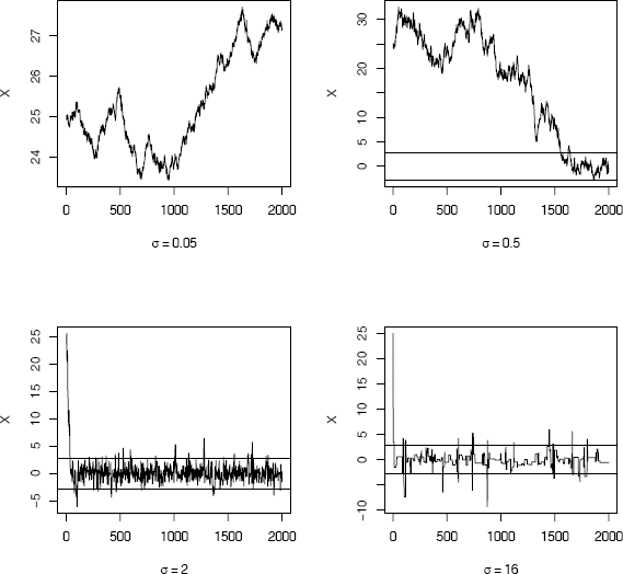
Random walk Metropolis chains generated by proposal distributions with different variances in Example 9.3.
In the first plot of Figure 9.3 with σ = 0.05, the ratios r(Xt, Y) tend to be large and almost every candidate point is accepted. The increments are small and the chain is almost like a true random walk. Chain 1 has not converged to the target in 2000 iterations. The chain in the second plot generated with σ = 0.5 is converging very slowly and requires a much longer burn-in period. In the third plot (σ = 2) the chain is mixing well and converging to the target distribution after a short burn-in period of about 500. Finally, in the fourth plot, where σ = 16, the ratios r(Xt, Y) are smaller and most of the candidate points are rejected. The fourth chain converges, but it is inefficient.
Example 9.4 (Example 9.3, cont.)
Usually in MCMC problems one does not have the theoretical quantiles of the target distribution available for comparison, but in this case the output of the random walk Metropolis chains in Example 9.3 can be compared with the theoretical quantiles of the target distribution. Discard the burn-in values in the first 500 rows of each chain. The quantiles are computed by the apply function (applying quantile to the columns of the matrix). The quantiles of the target distribution and the sample quantiles of the four chains rw1, rw2, rw3, and rw4 are in Table 9.1.
Quantiles of Target Distribution and Chains in Example 9.4.
Q |
rw1 |
rw2 |
rw3 |
rw4 |
|
|---|---|---|---|---|---|
5% |
−2.13 |
23.66 |
−1.16 |
−1.19 |
−2.40 |
10% |
−1.53 |
23.77 |
−0.39 |
−1.47 |
−1.35 |
20% |
−0.94 |
23.99 |
0.67 |
−1.01 |
−0.90 |
30% |
−0.57 |
24.29 |
4.15 |
−0.63 |
−0.64 |
40% |
−0.27 |
24.68 |
9.81 |
−0.25 |
−0.47 |
50% |
0.00 |
25.29 |
17.12 |
−0.01 |
−0.15 |
60% |
0.27 |
26.14 |
18.75 |
0.27 |
0.06 |
70% |
0.57 |
26.52 |
21.79 |
0.59 |
−0.25 |
80% |
0.94 |
26.93 |
25.42 |
0.92 |
0.52 |
90% |
1.53 |
27.27 |
28.51 |
1.55 |
1.18 |
95% |
2.13 |
27.39 |
29.78 |
2.37 |
1.90 |
a <- c(.05, seq(.1, .9, .1), .95)
Q <- qt(a, n)
rw <- cbind(rw1$x, rw2$x, rw3$x, rw4$x)
mc <- rw[501:N,]
Qrw <- apply(mc, 2, function(x) quantile(x, a))
print(round(cbind(Q, Qrw), 3)) #not shown
xtable::xtable(round(cbind(Q, Qrw), 3)) #latex format
R note 9.1 Table 9.1 was exported to LATEXformat by the xtable function in the xtable package [61].
Example 9.5 (Bayesian inference: A simple investment model)
In general, the returns on different investments are not independent. To reduce risk, portfolios are sometimes selected so that returns of securities are negatively correlated. Rather than the correlation of returns, here the daily performance is ranked. Suppose five stocks are tracked for 250 trading days (one year), and each day the “winner” is picked based on maximum return relative to the market. Let Xi be the number of days that security i is a winner. Then the observed vector of frequencies (x1, ... , x5) is an observation from the joint distribution of (X1, ... , X5). Based on historical data, suppose that the prior odds of an individual security being a winner on any given day are [1 : (1 − β) : (1 − 2β) : 2β : β], where β ∈ (0,0.5) is an unknown parameter. Update the estimate of β for the current year of winners.
According to this model, the multinomial joint distribution of X1, ... , X5 has the probability vector
p=(13,(1−β)3,(1−2β)3,2β3,β3).
The posterior distribution of β given (x1, ... , x5) is therefore
pr[β|(x1,...,x5)]=250!x1!x2!x3!x4!x5px11px22px33px44px55.
In this example, we cannot directly simulate random variates from the posterior distribution. One approach to estimating β is to generate a chain that converges to the posterior distribution and estimate β from the generated chain. Use the random walk Metropolis sampler with a uniform proposal distribution to generate the posterior distribution of β. The candidate point Y is accepted with probability
α(Xt,Y)=min(1,f(Y)f(Xt)).
The multinomial coefficient cancels from the ratio in α(X, Y), so that
The ratio can be further simplified, but the numerator and denominator are evaluated separately in the implementation below. In order to check the results, start by generating the observed frequencies from a distribution with specified β.
b <- .2 #actual value of beta
w <- .25 #width of the uniform support set
m <- 5000 #length of the chain
burn <- 1000 #burn-in time
days <- 250
x <- numeric(m) #the chain
# generate the observed frequencies of winners
i <- sample(1:5, size=days, replace=TRUE,
prob=c(1, 1-b, 1-2*b, 2*b, b))
win <- tabulate(i)
> print(win)
[1] 82 72 45 34 17
The tabulated frequencies in win are the simulated numbers of trading days that each of the stocks were the daily winner. Based on this year’s observed distribution of winners, we want to estimate the parameter β.
The following function prob computes the target density (without the constant).
prob <- function(y, win) {
# computes (without the constant) the target density
if (y < 0 || y >= 0.5)
return (0)
return((1/3)^win[1] *
((1-y)/3)^win[2] * ((1-2*y)/3)^win[3] *
((2*y)/3)^win[4] * (y/3)^win[5])
}
Finally the random walk Metropolis chain is generated. Two sets of uniform random variates are required; one for generating the proposal distribution and another for the decision to accept or reject the candidate point.
u <- runif(m) #for accept/reject step
v <- runif(m, -w, w) #proposal distribution
x[1] <- .25
for (i in 2:m) {
y <- x[i-1] + v[i]
if (u[i] <= prob(y, win) / prob(x[i-1], win))
x[i] <- y else
x[i] <- x[i-1]
}
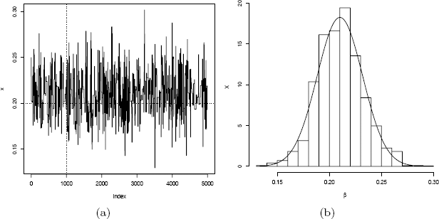
The plot of the chains in Figure 9.4(a) shows that the chain has converged, approximately, to the target distribution. Now the generated chain provides an estimate of β, after discarding a burn-in sample. From the histogram of the sample in Figure 9.4(b) the plausible values for β are close to 0.2.
The original sample table of relative frequencies, and the MCMC estimates of the multinomial probabilities are given below.
> print(win)
[1] 82 72 45 34 17
> print(round(win/days, 3))
[1] 0.328 0.288 0.180 0.136 0.068
> print(round(c(1, 1-b, 1-2*b, 2*b, b)/3, 3))
[1] 0.333 0.267 0.200 0.133 0.067
> xb <- x[(burn+1):m]
> print(mean(xb))
[1] 0.2101277
The sample mean of the generated chain is 0.2101277 (the simulated year of winners table was generated with β = 0.2). 0
9.2.4 The Independence Sampler
Another special case of the Metropolis-Hastings sampler is the independence sampler [272]. The proposal distribution in the independence sampling algorithm does not depend on the previous value of the chain. Thus, and the acceptance probability (9.3) is
The independence sampler is easy to implement and tends to work well when the proposal density is a close match to the target density, but otherwise does not perform well. Roberts [229] discusses convergence of the independence sampler, and comments that “it is rare for the independence sampler to be useful as a stand-alone algorithm.” Nevertheless, we illustrate the procedure in the following example, because the independence sampler can be useful in hybrid MCMC methods (see e.g. [119]).
Example 9.6 (Independence sampler)
Assume that a random sample (z1, ... , zn) from a two-component normal mixture is observed. The mixture is denoted by
and the density of the mixture (see Chapter 3) is
where f1 and f2 are the densities of the two normal distributions, respectively. If the densities f1 and f2 are completely specified, the problem is to estimate the mixing parameter p given the observed sample. Generate a chain using an independence sampler that has the posterior distribution of p as the target distribution.
The proposal distribution should be supported on the set of valid probabilities p; that is, the interval (0, 1). The most obvious choices are the beta distributions. With no prior information on p, one might consider the Beta(1,1) proposal distribution (Beta(1,1) is Uniform(0,1)). The candidate point Y is accepted with probability
where g(·) is the Beta proposal density. Thus, if the proposal distribution is Beta(a,b), then g(y) ∝ ya−1(1 − y)b−1 and Y is accepted with probability min(1, f(y)g(xt)/f(xt)g(y)), where
In the following simulation the proposal distribution is Uniform(0,1). The simulated data is generated from the normal mixture
The first steps are to initialize constants and generate the observed sample. Then an observed sample is generated. To generate the chain, all random numbers can be generated in advance because the candidate Y does not depend on Xt.
m <- 5000 #length of chain
xt <- numeric(m)
a <- 1 #parameter of Beta(a,b) proposal dist.
b <- 1 #parameter of Beta(a,b) proposal dist.
p <- .2 #mixing parameter
n <- 30 #sample size
mu <- c(0, 5) #parameters of the normal densities
sigma <- c(1, 1)
# generate the observed sample
i <- sample(1:2, size=n, replace=TRUE, prob=c(p, 1-p))
x <- rnorm(n, mu[i], sigma[i])
# generate the independence sampler chain
u <- runif(m)
y <- rbeta(m, a, b) #proposal distribution
xt[1] <- .5
for (i in 2:m) {
fy <- y[i] * dnorm(x, mu[1], sigma[1]) +
(1-y[i]) * dnorm(x, mu[2], sigma[2])
fx <- xt[i-1] * dnorm(x, mu[1], sigma[1]) +
(1-xt[i-1]) * dnorm(x, mu[2], sigma[2])
r <- prod(fy / fx) *
(xt[i-1]"(a-1) * (1-xt[i-1])"(b-1)) /
(y[i]"(a-1) * (1-y[i])"(b-1))
if (u[i] <= r) xt[i] <- y[i] else
xt[i] <- xt[i-1]
}
plot(xt, type="l", ylab="p")
hist(xt[101:m], main="", xlab="p", prob=TRUE)
print(mean(xt[101:m]))
The histogram of the generated sample after discarding the first 100 points is shown in Figure 9.5 on the next page. The mean of the remaining sample is 0.2516. The time plot of the generated chain is shown in Figure 9.6(a), which mixes well and converges quickly to a stationary distribution.

Distribution of the independence sampler chain for p with proposal distribution Beta(1, 1) in Example 9.6, after discarding a burn-in sample of length 100.

Chain generated by independence sampler for p with proposal distribution Beta(1, 1) (left) and Beta(5, 2) (right) in Example 9.6.
For comparison, we repeated the simulation with a Beta(5,2) proposal distribution. In this simulation the sample mean of the chain after discarding the burn-in sample is 0.2593, but the chain that is generated, shown in Figure 9.6(b) on the following page, is not very efficient.
9.3 The Gibbs Sampler
The Gibbs sampler was named by Geman and Geman [111], because of its application to analysis of Gibbs lattice distributions. However, it is a general method that can be applied to a much wider class of distributions [111, 106, 105]. It is another special case of the Metropolis-Hastings sampler. See the introduction to Gibbs sampling by Casella and George [40].
The Gibbs sampler is often applied when the target is a multivariate distribution. Suppose that all the univariate conditional densities are fully specified and it is reasonably easy to sample from them. The chain is generated by sampling from the marginal distributions of the target distribution, and every candidate point is therefore accepted.
Let X = (X1, ... , Xd) be a random vector in ℝd. Define the d − 1 dimensional random vectors
and denote the corresponding univariate conditional density of Xj given X(−j) by . The Gibbs sampler generates the chain by sampling from each of the d conditional densities .
In the following algorithm for the Gibbs sampler, we denote Xt by X(t).
- Initialize X(0) at time t = 0.
- For each iteration, indexed t = 1, 2, ... repeat:
- Set x1 = X1(t − 1).
- For each coordinate j = 1, ... ,d
- Generate from .
- Update .
- Set (every candidate is accepted).
- Increment t.
Example 9.7 (Gibbs sampler: Bivariate distribution)
Generate a bivariate normal distribution with mean vector (μ1, μ2), variances , and correlation ρ, using Gibbs sampling.
In the bivariate case, X = (X1, X2), X(−1) = X2,X(−2) = X1. The conditional densities of a bivariate normal distribution are univariate normal with parameters
and the chain is generated by sampling from
For a bivariate distribution (X1, X2), at each iteration the Gibbs sampler
- Sets (x1, x2) = X(t − 1);
- Generates from ;
- Updates
- Generates from ;
- Sets .
#initialize constants and parameters
N <- 5000 #length of chain
burn <- 1000 #burn-in length
X <- matrix(0, N, 2) #the chain, a bivariate sample
rho <- -.75 #correlation
mu1 <- 0
mu2 <- 2 sigma1 <- 1 sigma2 <- .5
s1 <- sqrt(1-rho^2)*sigma1
s2 <- sqrt(1-rho^2)*sigma2
###### generate the chain #####
X[1,] <- c(mu1, mu2) #initialize
for (i in 2:N) {
x2 <- X[i-1, 2]
m1 <- mu1 + rho * (x2 - mu2) * sigma1/sigma2
X[i, 1] <- rnorm(1, m1, s1) x1 <- X[i, 1]
m2 <- mu2 + rho * (x1 - mu1) * sigma2/sigma1
X[i, 2] <- rnorm(1, m2, s2)
}
b <- burn + 1
x <- X[b:N,]
The first 1000 observations are discarded from the chain in matrix X and the remaining observations are in x. Summary statistics for the column means, the sample covariance, and correlation matrices are shown below.
# compare sample statistics to parameters
>colMeans(x)
[1] -0.03030001 2.01176134
> cov(x)
[,1] [,2]
[1,] 1.0022207 -0.3757518
[2,] -0.3757518 0.2482327
> cor(x)
[,1] [,2]
[1,] 1.0000000 -0.7533379
[2,] -0.7533379 1.0000000
plot(x, main="", cex=.5, xlab=bquote(X[1]),
ylab=bquote(X[2]), ylim=range(x[,2]))
The sample means, variances, and correlation are close to the true parameters, and the plot in Figure 9.7 exhibits the elliptical symmetry of the bivariate normal, with negative correlation. (The version printed is a randomly selected subset of 1000 generated variates after discarding the burn-in sample.)

9.4 Monitoring Convergence
In several examples using various Metropolis-Hastings algorithms, we have seen that some generated chains have not converged to the target distribution. In general, for an arbitrary Metropolis-Hastings sampler the number of iterations that are sufficient for approximate convergence to the target distribution or what length burn-in sample is required are unknown. Moreover, Gelman and Rubin [110] provide examples of slow convergence that cannot be detected by examining a single chain. A single chain may appear to have converged because the generated values have a small variance within a local part of the support set of the target distribution, but in reality the chain has not explored all of the support set. By examining several parallel chains, slow convergence should be more evident, particularly if the initial values of the chain are overdispersed with respect to the target distribution. Methods have been proposed in the literature for monitoring the convergence of MCMC chains (see e.g. [33, 54, 116, 138, 227, 219]). In this section we discuss and illustrate the approach suggested by Gelman and Rubin [107, 109] for monitoring convergence of Metropolis-Hastings chains.
9.4.1 The Gelman-Rubin Method
The Gelman-Rubin [107, 109] method of monitoring convergence of a M-H chain is based on comparing the behavior of several generated chains with respect to the variance of one or more scalar summary statistics. The estimates of the variance of the statistic are analogous to estimates based on between-sample and within-sample mean squared errors in a one-way analysis of variance (ANOVA).
Let ψ be a scalar summary statistic that estimates some parameter of the target distribution. Generate k chains {Xij : 1 ≤ i ≤ k, 1 ≤ j ≤ n }of length n. (Here the chains are indexed with initial time t = 1.) Compute {ψin = ψ(Xi1, ..., Xin)} for each chain at time n. We expect that if the chains are converging to the target distribution as n → ∞, then the sampling distribution of the statistics {ψin} should be converging to a common distribution.
The Gelman-Rubin method uses the between-sequence variance of ψ and the within-sequence variance of ψ to estimate an upper bound and a lower bound for variance of ψ, converging to variance ψ from above and below, respectively, as the chain converges to the target distribution.
Consider the chains up to time n to represent data from a balanced one-way ANOVA on k groups with n observations. Compute the estimates of between-sample and within-sample variance analogous to the sum of squares for treatments and the sum of squares for error, and the corresponding mean squared errors as in ANOVA.
The between-sequence variance is
where
Within the ith sequence, the sample variance is
and the pooled estimate of within sample variance is
The between-sequence and within-sequence estimates of variance are combined to estimate an upper bound for Var(ψ)
If the chains were random samples from the target distribution, (9.5) is an unbiased estimator of Var(ψ). In this application (9.5) is positively biased for the variance of ψ if the initial values of the chain are over-dispersed, but converges to Var(ψ) as n → ∞. On the other hand, if the chains have not converged by time n, the chains have not yet mixed well across the entire support set of the target distribution so the within-sample variance W underestimates the variance of ψ. As n → ∞ we have the expected value of (9.5) converging to Var(ψ) from above and W converging to Var(ψ) from below. If is large relative to W this suggests that the chain has not converged to the target distribution by time n.
The Gelman-Rubin statistic is the estimated potential scale reduction
which can be interpreted as measuring the factor by which the standard deviation of ψ could be reduced by extending the chain. The factor decreases to 1 as the length of the chain tends to infinity, so should be close to 1 if the chains have approximately converged to the target distribution. Gelman [107] suggests that should be less than 1.1 or 1.2.
Example 9.8 (Gelman-Rubin method of monitoring convergence)
This example illustrates the Gelman-Rubin method of monitoring convergence of a Metropolis chain. The target distribution is Normal(0,1), and the proposal distribution is Normal(Xt, σ2). The scalar summary statistic ψij is the mean of the ith chain up to time j. After generating all chains the diagnostic statistics are computed in the Gelman.Rubin function below.
Gelman.Rubin <- function(psi) {
# psi[i,j] is the statistic psi(X[i,1:j])
# for chain in i-th row of X
psi <- as.matrix(psi)
n <- ncol(psi)
k <- nrow(psi)
psi.means <- rowMeans(psi) #row means
B <- n * var(psi.means) #between variance est.
psi.w <- apply(psi, 1, "var") #within variances
W <- mean(psi.w) #within est.
v.hat <- W*(n-1)/n + (B/n) #upper variance est.
r.hat <- v.hat / W #G-R statistic
return(r.hat)
}
Since several chains are to be generated, the M-H sampler is written as a function normal.chain.
normal.chain <- function(sigma, N, X1) {
#generates a Metropolis chain for Normal(0,1)
#with Normal(X[t], sigma) proposal distribution
#and starting value X1
x <- rep(0, N)
x[1] <- X1
u <- runif(N)
for (i in 2:N) {
xt <- x[i-1]
y <- rnorm(1, xt, sigma) #candidate point
r1 <- dnorm(y, 0, 1) * dnorm(xt, y, sigma)
r2 <- dnorm(xt, 0, 1) * dnorm(y, xt, sigma)
r <- r1 / r2
if (u[i] <= r) x[i] <- y else
x[i] <- xt
}
return(x)
}
In the following simulation, the proposal distribution has a small variance σ2 = 0.04. When the variance is small relative to the target distribution, the chains are usually converging slowly.
sigma <- .2 #parameter of proposal distribution
k <- 4 #number of chains to generate
n <- 15000 #length of chains
b <- 1000 #burn-in length
#choose overdispersed initial values
x0 <- c(-10, -5, 5, 10)
#generate the chains
X <- matrix(0, nrow=k, ncol=n)
for (i in 1:k)
X[i,] <- normal.chain(sigma, n, x0[i])
#compute diagnostic statistics
psi <- t(apply(X, 1, cumsum))
for (i in 1:nrow(psi))
psi[i,] <- psi[i,] / (1:ncol(psi))
print(Gelman.Rubin(psi))
#plot psi for the four chains
par(mfrow=c(2,2))
for (i in 1:k)
plot(psi[i, (b+1):n], type="l",
xlab=i, ylab=bquote(psi))
par(mfrow=c(1,1)) #restore default
#plot the sequence of R-hat statistics
rhat <- rep(0, n)
for (j in (b+1):n)
rhat[j] <- Gelman.Rubin(psi[,1:j])
plot(rhat[(b+1):n], type="l", xlab="", ylab="R")
abline(h=1.1, lty=2)
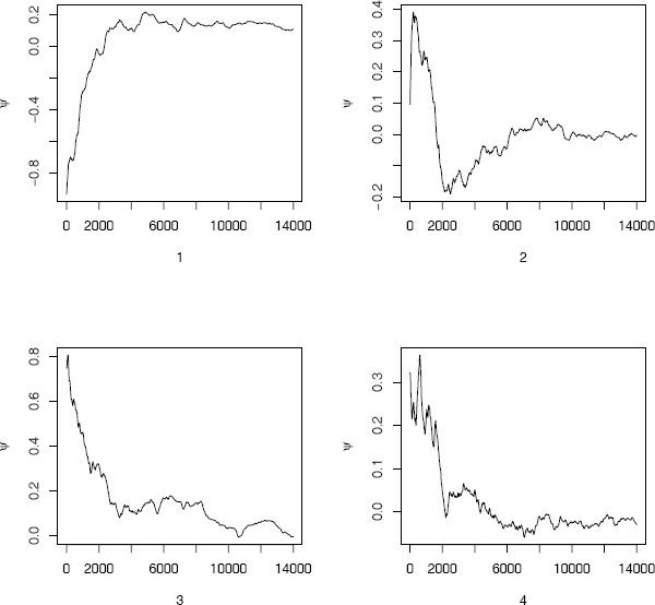
The plots of the four sequences of the summary statistic (the mean) ψ are shown in Figure 9.8 from time 1001 to 15000. Rather than interpret the plots, one can refer directly to the value of the factor to monitor convergence. The value at time n = 5000 suggests that the chain should be extended. The plot of (Figure 9.9(a)) over time 1001 to 15000 suggests that the chain has approximately converged to the target distribution within approximately 10000 iterations . The dashed line on the plot is at . Some intermediate values are 1.2252, 1.1836, 1.1561, and 1.1337 at times 6000, 7000, 8000, and 9000, respectively. The value of is less than 1.1 within time 11200.
For comparison the simulation is repeated, where the variance of the proposal distribution is σ2 = 4. The plot of is shown in Figure 9.9(b) for time 1001 to 15000. From this plot it is evident that the chain is converging faster than when the proposal distribution had a very small variance. The value of is below 1.2 within 2000 iterations and below 1.1 within 4000 iterations.

Sequence of the Gelman-Rubin for four Metropolis-Hastings chains in Example 9.8 (a) σ = 0.2, (b) σ = 2.
9.5 Application: Change Point Analysis
A Poisson process is often chosen to model the frequency of rare events. Poisson processes are discussed in Section 3.7. A homogeneous Poisson process {X(t), t ≥ 0} with constant rate λ is a counting process with independent and stationary increments, such that X(0) = 0 and the number of events X(t) in [0, t] has the Poisson(λt) distribution.
Suppose that the parameter λ, which is the expected number of events that occur in a unit of time, has changed at some point in time k. That is, Xt ~ Poisson(μt) for 0 < t ≤ k and Xt ~ Poisson(λt) for k < t. Given a sample of n observations from this process, the problem is to estimate μ, λ and k.
For a specific application, consider the following well known example. The coal data in the boot package [34] gives the dates of 191 explosions in coal mines which resulted in 10 or more fatalities from March 15, 1851 until March 22, 1962. The data are given in [126], originally from [153]. This problem has been discussed by many authors, including e.g. [36, 37, 63, 121, 171, 192]. A Bayesian model and Gibbs sampling can be applied to estimate the change point in the annual number of coal mining disasters.
Example 9.9 (Coal mining disasters)
In the coal data, the date of the disaster is given. The integer part of the date gives the year. For simplicity truncate the fractional part of the year. As a first step, tabulate the number of disasters per year and create a time plot.
library(boot) #for coal data
data(coal)
year <- floor(coal)
y <- table(year)
plot(y) #a time plot
From the plot in Figure 9.10 it appears that a change in the average number of disasters per year may have occurred somewhere around the turn of the century. Note that vector of frequencies returned by Table omits the years where there are zero counts, so for the change point analysis tabulate is applied.

y <- floor(coal[[1]])
y <- tabulate(y)
y <- y[1851:length(y)]
Sequence of annual number of coal mining disasters:
4 5 4 1 0 4 3 4 0 6 3 3 4 0 2 6 3 3 5 4 5 3 1 4 4
1 5 5 3 4 2 5 2 2 3 4 2 1 3 2 2 1 1 1 1 3 0 0 1 0
1 1 0 0 3 1 0 3 2 2 0 1 1 1 0 1 0 1 0 0 0 2 1 0 0
0 1 1 0 2 3 3 1 1 2 1 1 1 1 2 3 3 0 0 0 1 4 0 0 0
1 0 0 0 0 0 1 0 0 1 0 1
Let Yi be the number of disasters in year i, where 1851 is year 1. Assume that the change point occurs at year k, and the number of disasters in year i is a Poisson random variable, where
There are n = 112 observations ending with year 1962.
Assume the Bayesian model with independent priors
introducing additional parameters b1 and b2, independently distributed as a positive multiple of a chisquare random variable. That is,
Let and To apply the Gibbs sampler, the fully specified conditional distributions are needed. The conditional distributions for μ, λ, b1, and b2 are given by
and the posterior density of the change point k is
where
is the likelihood function.
For the change point analysis with the model specified on the previous page, the Gibbs sampler algorithm is as follows (G(a, b) denotes the Gamma(shape= a, rate= b) distribution).
- Initialize k by a random draw from 1:n, and initialize λ, μ, b1, b2 to 1.
- For each iteration, indexed t = 1, 2,... repeat:
- Generate μ(t) from G(0.5 + Sk(t−1), k(t − 1) + b1(t − 1)).
- Generate λ(t) from .
- Generate b1(t) from G(0.5, μ(t) + 1).
- Generate b2(t) from G(0.5, λ(t) + 1).
- Generate k(t) from the multinomial distribution defined by (9.7) using the updated values of λ, μ, b1, b2.
- X(t) = (μ(t), λ(t), b1(t), b2(t), k(t)) (every candidate is accepted).
- Increment t.
The implementation of the Gibbs sampler for this problem is shown on the facing page.
From the output of the Gibbs sampler below, the following sample means are obtained after discarding a burn-in sample of size 200. The estimated change point is k≐ 40. From year k = 1 (1851) to k = 40 (1890) the estimated Poisson mean is and from year k = 41 (1891) forward the estimated Poisson mean is
b <- 201
j <- k[b:m]
> print(mean(k[b:m]))
[1] 39.935
> print(mean(lambda[b:m]))
[1] 0.9341033
> print(mean(mu[b:m]))
[1] 3.108575
Histograms and plots of the chains are shown in Figures 9.11 and 9.12. Code to generate the plots is given on page 279.


Distribution of μ, λ, and k from the change point analysis for coal mining disasters in Example 9.9.
# Gibbs sampler for the coal mining change point
# initialization
n <- length(y) #length of the data
m <- 1000 #length of the chain
mu <- lambda <- k <- numeric(m)
L <- numeric(n)
k[1] <- sample(1:n, 1)
mu[1] <- 1
lambda[1] <- 1
b1 <- 1
b2 <- 1
# run the Gibbs sampler
for (i in 2:m) {
kt <- k[i-1]
#generate mu
r <- .5 + sum(y[1:kt])
mu[i] <- rgamma(1, shape = r, rate = kt + b1)
#generate lambda
if (kt + 1 > n) r <- .5 + sum(y) else
r <- .5 + sum(y[(kt+1):n])
lambda[i] <- rgamma(1, shape = r, rate = n - kt + b2)
#generate b1 and b2
b1 <- rgamma(1, shape = .5, rate = mu[i]+1)
b2 <- rgamma(1, shape = .5, rate = lambda[i]+1)
for (j in 1:n) {
L[j] <- exp((lambda[i] - mu[i]) * j) *
(mu[i] / lambda[i])^sum(y[1:j])
}
L <- L / sum(L)
#generate k from discrete distribution L on 1:n
k[i] <- sample(1:n, prob=L, size=1)
}
Several contributed packages for R offer implementations of the methods in this chapter. See, for example, the packages mcmc and MCMCpack [117, 191]. The coda (Convergence Diagnosis and Output Analysis) package [212] provides utilities that summarize, plot, and diagnose convergence of mcmc objects created by functions in MCMCpack. Also see mcgibbsit [291]. For implementation of Bayesian methods in general, see the task view on CRAN “Bayesian Inference” for a description of several packages.
Exercises
9.1 Repeat Example 9.1 for the target distribution Rayleigh(σ = 2). Compare the performance of the Metropolis-Hastings sampler for Example 9.1 and this problem. In particular, what differences are obvious from the plot corresponding to Figure 9.1?
9.2 Repeat Example 9.1 using the proposal distribution Y ~ Gamma(Xt,1) (shape parameter Xt and rate parameter 1).
9.3 Use the Metropolis-Hastings sampler to generate random variables from a standard Cauchy distribution. Discard the first 1000 of the chain, and compare the deciles of the generated observations with the deciles of the standard Cauchy distribution (see qcauchy or qt with df=1). Recall that a Cauchy(θ, η) distribution has density function
The standard Cauchy has the Cauchy(θ = 1, η = 0) density. (Note that the standard Cauchy density is equal to the Student t density with one degree of freedom.)
9.4 Implement a random walk Metropolis sampler for generating the standard Laplace distribution (see Exercise 3.2). For the increment, simulate from a normal distribution. Compare the chains generated when different variances are used for the proposal distribution. Also, compute the acceptance rates of each chain.
9.5 What effect, if any, does the width w have on the mixing of the chain in Example 9.5? Repeat the simulation keeping the random number seed fixed, trying different proposal distributions based on the random increments from Uniform(—w, w), varying w.
9.6 Rao [220, Sec. 5g] presented an example on genetic linkage of 197 animals in four categories (also discussed in [67, 106, 171, 266]). The group sizes are (125,18, 20, 34). Assume that the probabilities of the corresponding multinomial distribution are
Estimate the posterior distribution of θ given the observed sample, using one of the methods in this chapter.
9.7 Implement a Gibbs sampler to generate a bivariate normal chain (Xt, Yt) with zero means, unit standard deviations, and correlation 0.9. Plot the generated sample after discarding a suitable burn-in sample. Fit a simple linear regression model Y = β0 + β1X to the sample and check the residuals of the model for normality and constant variance.
9.8 This example appears in [40]. Consider the bivariate density
It can be shown (see e.g. [23]) that for fixed a, b, n, the conditional distributions are Binomial(n, y) and Beta(x + a, n − x + b). Use the Gibbs sampler to generate a chain with target joint density f(x, y).
9.9 Modify the Gelman-Rubin convergence monitoring given in Example 9.8 so that only the final value of is computed, and repeat the example, omitting the graphs.
9.10 Refer to Example 9.1. Use the Gelman-Rubin method to monitor convergence of the chain, and run the chain until the chain has converged approximately to the target distribution according to (See Exercise 9.9.) Also use the coda [212] package to check for convergence of the chain by the Gelman-Rubin method. Hints: See the help topics for the coda functions gelman.diag, gelman.plot, as.mcmc, and mcmc.list.
9.11 Refer to Example 9.5. Use the Gelman-Rubin method to monitor convergence of the chain, and run the chain until the chain has converged approximately to the target distribution according to Also use the coda [212] package to check for convergence of the chain by the Gelman-Rubin method. (See Exercises 9.9 and 9.10.)
9.12 Refer to Example 9.6. Use the Gelman-Rubin method to monitor convergence of the chain, and run the chain until the chain has converged approximately to the target distribution according to Also use the coda [212] package to check for convergence of the chain by the Gelman-Rubin method. (See Exercises 9.9 and 9.10.)
R Code
Code for Figure 9.3 on page 255
Reference lines are added at the t0.025(ν) and t0.975(ν) quantiles.
par(mfrow=c(2,2)) #display 4 graphs together
refline <- qt(c(.025, .975), df=n)
rw <- cbind(rw1$x, rw2$x, rw3$x, rw4$x)
for (j in 1:4) {
plot(rw)[,j], type="l",
xlab=bquote(sigma == .(round(sigma[j],3))),
ylab="X", ylim=range(rw[,j]))
abline(h=refline)
}
par(mfrow=c(1,1)) #reset to default
Code for Figures 9.4(a) on page 259 and 9.4(b) on page 259
plot(x, type="l")
abline(h=b, v=burn, lty=3)
xb <- x[- (1:burn)]
hist(xb, prob=TRUE, xlab=bquote(beta), ylab="X", main="")
z <- seq(min(xb), max(xb), length=100)
lines(z, dnorm(z, mean(xb), sd(xb)))
Code for Figure 9.11 on page 276
# plots of the chains for Gibbs sampler output
par(mfcol=c(3,1), ask=TRUE)
plot(mu, type="l", ylab="mu")
plot(lambda, type="l", ylab="lambda")
plot(k, type="l", ylab="change point = k")
Code for Figure 9.12 on page 276
# histograms from the Gibbs sampler output
par(mfrow=c(2,3))
labelk <- "changepoint"
label1 <- paste("mu", round(mean(mu[b:m]), 1))
label2 <- paste("lambda", round(mean(lambda[b:m]), 1))
hist(mu[b:m], main="", xlab=label1,
breaks = "scott", prob=TRUE) #mu posterior
hist(lambda[b:m], main="", xlab=label2,
breaks = "scott", prob=TRUE) #lambda posterior
hist(j, breaks=min(j):max(j), prob=TRUE, main="",
xlab = labelk)
par(mfcol=c(1,1), ask=FALSE) #restore display