
3.7. A MATRIX DECOMPOSITION 63
is an XU(4) matrix.
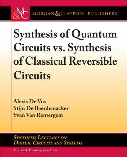
If n > 2, then XU(n) has more dimensions than ZU(n), as .n 1/
2
exceeds n 1. See
Figure 3.2. erefore, a conjugation property like (3.11) is not possible. Instead, we have that
ZU.n/ F
1
XU.n/ F and XU.n/ F ZU.n/ F
1
:
In particular, the group F ZU.n/ F
1
is the subgroup of XU(n) consisting of all circulant XU(n)
matrices. Indeed, if a matrix C equals FDF
1
, with D some n n diagonal matrix, then the
matrix entry
C
jk
D
X
r
X
s
F
jr
D
rs
.F
1
/
sk
D
X
r
F
jr
D
rr
.F
1
/
rk
D
1
n
X
r
!
.j 1/.r1/
D
rr
!
.r1/.k1/
D
1
n
X
r
!
.j k/.r1/
D
rr
is a number dependent only on the difference j k. We will denote the group of circulant XU(n)
matrices cXU(n). It is isomorphic to ZU(n) and thus has dimension n 1.
U(?)
1
XU(?) ZU(?) ∞
(?–1)
2
∞
?–1
1(?)
∞
?
2
Figure 3.2: Hierarchy of the Lie groups U(n), XU(n), ZU(n), and the finite group 1(n).
3.7 A MATRIX DECOMPOSITION
An important theorem is the ZXZ theorem: any U(n) matrix U can be decomposed as
U D e
i˛
Z
1
XZ
2
; (3.14)
where both Z
1
and Z
2
are ZU(n) matrices and X is an XU(n) matrix. e decomposi-
tion is a generalization of (3.6) for n larger than 2. It was conjectured by De Vos and De
Baerdemacker [51] and subsequently proved by Idel and Wolf [58]. e proof of the theorem
is based on symplectic topology. e proof is not constructive. at means that we know there

64 3. BOTTOM-UP
exists a set f˛; Z
1
; X; Z
2
g, but (for n > 2) we presently lack a general method to find, for a given
matrix U , the corresponding number ˛ and matrices Z
1
, X, and Z
2
.
For some particular (simple) cases, the analytical decomposition is known. For example, if
n D 2, then the arbitrary unitary matrix, as given by (1.14), has two ZXZ decompositions, given
by (3.6)–(3.7)–(3.8). is illustrates that the ZXZ decomposition is not necessarily unique.
If n > 2, then we can recur to a numerical iterative algorithm to find (one of) the decom-
position(s) with arbitrary precision [51]. For example, the 3 3 unitary matrix
1
4
0
@
1 1 3i 2 Ci
1 3i 2 1 C i
2 C i 1 i 3
1
A
;
yields, after only five iterations, a ZXZ decomposition with the following X factor:
0
@
0:2398 C 0:0708 i 0:7522 C 0:2432 i 0:4337 0:3527 i
0:7113 0:3451 i 0:4945 C 0:0739 i 0:2341 C 0:2649 i
0:4871 C 0:2742 i 0:1564 0:3171 i 0:7448 C0:0878 i
1
A
:
e reader may verify that all six line sums are close to unity. e algorithm is based on a
Sinkhorn-like [59] procedure, where the given U(n) matrix is repeatedly left multiplied and
right multiplied with a diagonal unitary, until the product approximates an XU(n) matrix suffi-
ciently closely.
We remark that the ZXZ decomposition of a unitary matrix is reminiscent of the HVH
decomposition (1.9) of a permutation. As in Section 1.8, we can mention three theorems.
eorem 3.1 Each unitary matrix U can be decomposed as
U D D
1
XD
2
; (3.15)
where both D
1
and D
2
are diagonal unitary matrices and X is a unit-linesum unitary matrix.
eorem 3.2 e ZXZ theorem is a decomposition of the form (3.15), e
i˛
Z
1
playing the role of D
1
and Z
2
playing the role of D
2
.
is theorem is slightly more powerful than eorem 3.1, as the upper-left entry of D
2
is allowed to be equal to 1.
eorem 3.3 In the ZXZ decomposition (3.14), the scalar e
i˛
commutes with the matrix Z
1
X,
yielding a (3.15) decomposition, where Z
1
plays the role of D
1
and e
i˛
Z
2
plays the role of D
2
.
Also, this theorem is slightly more powerful than eorem 3.1, as now the upper-left
entry of D
1
is allowed to be equal to 1.
..................Content has been hidden....................
You can't read the all page of ebook, please click here login for view all page.