
Chapter 36
Statistical Aggregate Functions
“Its not that figures lie, its that liars figure.”
Table of Contents Chapter 36 – Statistical Aggregate Functions
– Another CORR Example so you can Compare
– Another COVAR_POP Example so you can Compare
– Another REGR_INTERCEPT Example so you can Compare
– Another REGR_SLOPE Example so you can Compare
– No Having Clause Vs Use of HAVING
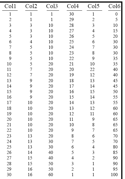
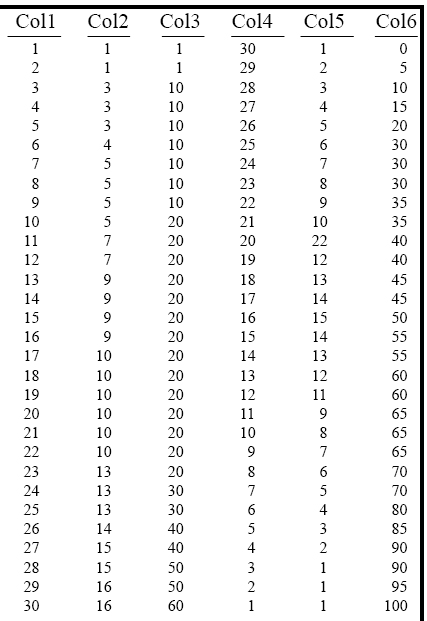
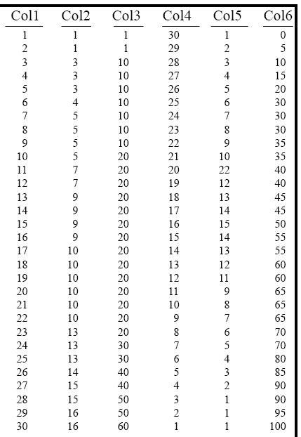
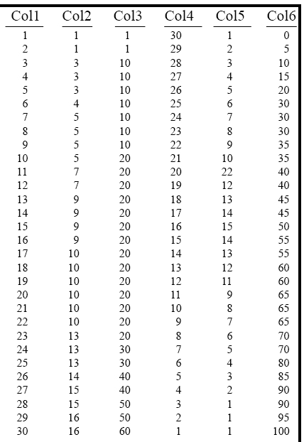
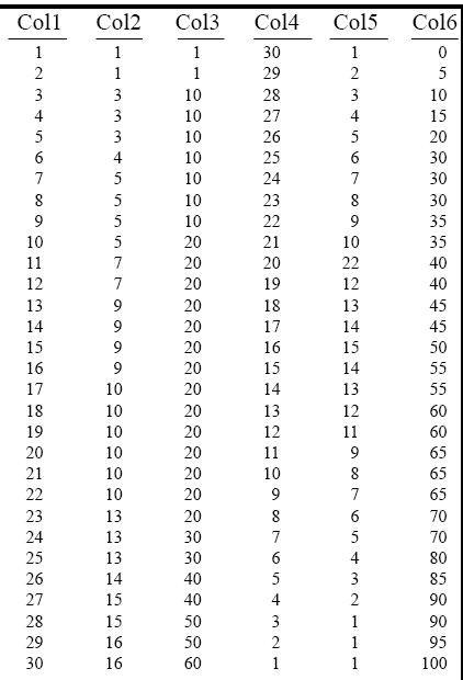
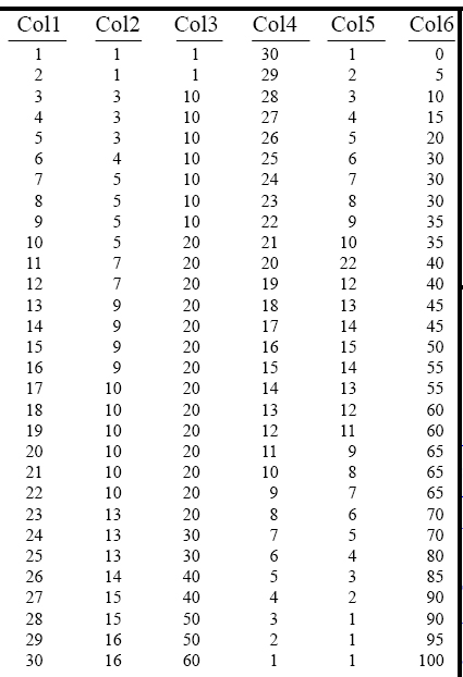
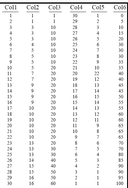
The Stats Table

Above is the Stats_Table data in which we will use in our statistical examples.
The KURTOSIS Function
SELECT KURTOSIS(col1) AS KofCol1
FROM Stats_Table;
The KURTOSIS function is used to return a number that represents the sharpness of a peak on a plotted curve of a probability function for a distribution compared with the normal distribution.
A high value result is referred to as leptokurtic. While a medium result is referred to as mesokurtic and a low result is referred to as platykurtic.
A positive value indicates a sharp or peaked distribution and a negative number represents a flat distribution. A peaked distribution means that one value exists more often than the other values. A flat distribution means there is the same quantity values exist for each number.
If you compare this to the row distribution associated within Teradata, most of the time a flat distribution is best, with the same number of rows stored on each AMP. Having skewed data represents more of a lumpy distribution.
A Kurtosis Example
Stats_Table

SELECT KURTOSIS(col1) AS KofCol1
,KURTOSIS(col2) AS KofCol2
,KURTOSIS(col3) AS KofCol3
,KURTOSIS(col4) AS KofCol4
,KURTOSIS(col5) AS KofCol5
,KURTOSIS(col6) AS KofCol6
FROM Stats_Table;
![]()
The SKEW Function
SELECT SKEW(col1) AS SKofCol1
FROM Stats_Table;
The Skew indicates that a distribution does not have equal probabilities above and below the mean (average). In a skew distribution, the median and the mean are not coincident, or equal.
Where:
– a median value < mean value = a positive skew
– a median value > mean value = a negative skew
– a median value = mean value = no skew
Syntax for using SKEW:
SKEW(<column-name>)
A SKEW Example
Stats_Table
SELECT SKEW(col1) AS SKofCol1
,SKEW(col2) AS SKofCol2
,SKEW(col3) AS SKofCol3
,SKEW(col4) AS SKofCol4
,SKEW(col5) AS SKofCol5
,SKEW(col6) AS SKofCol6
FROM Stats_Table;
![]()
A median value < mean value = a positive skew
A median value > mean value = a negative skew
A median value = mean value = no skew
The STDDEV_POP Function
SELECT STDDEV_POP(col1) AS SDPCol1
FROM Stats_Table;
The standard deviation function is a statistical measure of spread or dispersion of values. It is the root's square of the difference of the mean (average). This measure is to compare the amount by which a set of values differs from the arithmetical mean.
The STDDEV_POP function is one of two that calculates the standard deviation. The population is of all the rows included based on the comparison in the WHERE clause.
Syntax for using STDDEV_POP:
STDDEV_POP(<column-name>)
A STDDEV_POP Example
Stats_Table
SELECT STDDEV_POP(col1) AS SDPCol1
,STDDEV_POP(col2) AS SDPCol2
,STDDEV_POP(col3) AS SDPCol3
,STDDEV_POP(col4) AS SDPCol4
,STDDEV_POP(col5) AS SDPCol5
,STDDEV_POP(col6) AS SDPCol6
FROM Stats Table;
![]()
The standard deviation function is a statistical measure of spread or dispersion of values. It is the root's square of the difference of the mean (average). This measure is to compare the amount by which a set of values differs from the arithmetical mean.
The STDDEV_SAMP Function
SELECT STDDEV_SAMP(col1) AS SDSCol1
FROM Stats_Table;
The standard deviation Unction is a statistical measure of spread or dispersion of values. It is the root's square of the difference of the mean (average). This measure is to compare the amount by which a set of values differs from the arithmetical mean.
The STDDEV_SAMP function is one of two that calculates the standard deviation. The sample is a random selection of all rows returned based on the comparisons in the WHERE clause. The population is for all of the rows based on the WHERE clause.
Syntax for using STDDEV_SAMP:
STDDEV_SAMP(<column-name>)
A STDDEV_SAMP Example
Stats_Table

SELECT STDDEV_POP(col1) AS SDSCol1
,STDDEV_POP(col2) AS SDSCol2
,STDDEV_POP(col3) AS SDSCol3
,STDDEV_POP(col4) AS SDSCol4
,STDDEV_POP(col5) AS SDSCol5
,STDDEV_POP(col6) AS SDSCol6
FROM Stats Table;
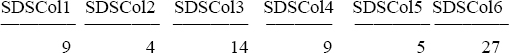
The STDDEV_SAMP function is one of two that calculates the standard deviation. The sample is a random selection of all rows returned based on the comparisons in the WHERE clause. The population is for all of the rows based on the WHERE clause.
The VAR_POP Function
SELECT VAR_POP(col1) AS VPCol1
FROM Stats_Table;
The Variance Unction is a measure of dispersion (spread of the distribution) as the square of the standard deviation. There are two forms of Variance in Teradata, VAR_POP is for the entire population of data rows allowed by the WHERE clause.
Although standard deviation and variance are regularly used in statistical calculations, the meaning of variance is not easy to elaborate. Most often variance is used in theoretical work where a variance of the sample is needed.
There are two methods for using variance. These are the Kruskal-Wallis one-way Analysis of Variance and Friedman two-way Analysis of Variance by rank.
Syntax for using VAR_POP:
VAR_POP(<column-name>)
A VAR_POP Example
Stats_Table
SELECT VAR_POP(col1) AS VPCol1
,VAR_POP(col2) AS VPCol2
,VAR_POP(col3) AS VPCol3
,VAR_POP(col4) AS VPCol4
,VAR_POP(col5) AS VPCol5
,VAR_POP(col6) AS VPCol6
FROM Stats Table;
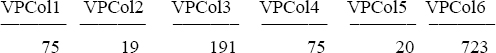
The Variance function is a measure of dispersion (spread of the distribution) as the square of the standard deviation. There are two forms of Variance in Teradata, VAR_POP is for the entire population of data rows allowed by the WHERE clause.
The VAR_SAMP Function
SELECT VAR_SAMP(col1) AS VSCol1
FROM Stats_Table;
The Variance function is a measure of dispersion (spread of the distribution) as the square of the standard deviation. There are two forms of Variance in Teradata, VAR_SAMP is used for a random sampling of the data rows allowed through by the WHERE clause.
Although standard deviation and variance are regularly used in statistical calculations, the meaning of variance is not easy to elaborate. Most often variance is used in theoretical work where a variance of the sample is needed to look for consistency.
There are two methods for using variance. These are the Kruskal-Wallis one-way Analysis of Variance and Friedman two-way Analysis of Variance by rank. Syntax for using VAR_SAMP:
VAR_SAMP(<column-name>)
A VAR_SAMP Example
Stats_Table
SELECT VAR_SAMP(col1) AS VSCol1
,VAR_SAMP(col2) AS VSCol2
,VAR_SAMP(col3) AS VSCol3
,VAR_SAMP(col4) AS VSCol4
,VAR_SAMP(col5) AS VSCol5
,VAR_SAMP(col6) AS VSCol6
FROM Stats Table ;
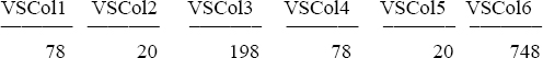
The Variance function is a measure of dispersion (spread of the distribution) as the square of the standard deviation. There are two forms of Variance in Teradata, VAR_SAMP is used for a random sampling of the data rows allowed through by the WHERE clause.
The CORR Function
SELECT CORR(col1, col2) AS CCol1#2
FROM Stats_Table;
The CORR function is a binary function, meaning that two variables are used as input to it. It measures the association between 2 random variables. If the variables are such that when one changes the other does so in a related manner, they are correlated. Independent variables are not correlated because the change in one does not necessarily cause the other to change.
The correlation coefficient is a number between –1 and 1. It is calculated from a number of pairs of observations or linear points (X,Y).
Where:
1 = perfect positive correlation
0 = no correlation
-1 = perfect negative correlation
Syntax for using CORR:
CORR(<column-name>, <column-name>)
A CORR Example
Stats_Table

SELECT CORR(col1, col2) AS CCol1#2
,CORR(col1, col3) AS CCol1#3
,CORR(col1, col4) AS CCol1#4
,CORR(col1, col5) AS CCol1#5
,CORR(col1, col6) AS CCol1#6
FROM Stats Table ;

Where:
1 = perfect positive correlation
0 = no correlation
–1 = perfect negative correlation
Another CORR Example so you can Compare
Stats_Table

SELECT CORR(col4, col2) AS CCol4#2
,CORR(col4, col3) AS CCol4#3
,CORR(col4, col1) AS CCol4#1
,CORR(col4, col5) AS CCol4#5
,CORR(col4, col6) AS CCol4#6
FROM Stats Table ;

Where:
1 = perfect positive correlation
0 = no correlation
–0.991612
The COVAR_POP Function
SELECT COVAR_POP(col1, col2) AS CCol1#2
FROM Stats_Table;
The covariance is a statistical measure of the tendency of two variables to change in conjunction with each other. It is equal to the product of their standard deviations and correlation coefficients.
The covariance is a statistic used for bivariate samples or bivariate distribution. It is used for working out the equations for regression lines and the product-moment correlation coefficient.
Syntax:
COVAR(<column-name>, <column-name>)
A COVAR_POP Example
Stats_Table

SELECT
COVAR_POP(col1, col2) AS CPCol1#2
,COVAR_POP(col1, col3) AS CPCol1#3
,COVAR_POP(col1, col4) AS CPCol1#4
,COVAR_POP(col1, col5) AS CPCol1#5
,COVAR_POP(col1, col6) AS CPCol1#6
FROM Stats_Table ;
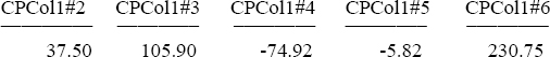
The covariance is a statistical measure of the tendency of two variables to change in conjunction with each other. It is equal to the product of their standard deviations and correlation coefficients.
Another COVAR_POP Example so you can Compare
Stats_Table

SELECT
COVAR_POP(col4, col2) AS CPCol4#2
,COVAR_POP(col4, col3) AS CPCol4#3
,COVAR_POP(col4, col1) AS CPCol4#1
,COVAR_POP(col4, col5) AS CPCol4#5
,COVAR_POP(col4, col6) AS CPCol4#6
FROM Stats_Table ;
The covariance is a statistical measure of the tendency of two variables to change in conjunction with each other. It is equal to the product of their standard deviations and correlation coefficients.
The REGR_INTERCEPT Function
SELECT REGR_INTERCEPT(col1, col2) AS RIofCol1#2
FROM Stats_Table;
A regression line is a line of best fit, drawn through a set of points on a graph for X and Y coordinates. It uses the Y coordinate as the Dependent Variable and the X value as the Independent Variable.
Two regression lines always meet or intercept at the mean of the data points(x,y), where x=AVG(x) and y=AVG(y) and is not usually one of the original data points.
Syntax for using REGR_INTERCEPT:
REGR_INTERCEPT(dependent-expression, independent-expression)
A REGR_INTERCEPT Example
Stats_Table

SELECT
REGR_INTERCEPT(col1, col2) AS RICol1#2
,REGR_INTERCEPT(col1, col3) AS RICol1#3
,REGR_INTERCEPT(col1, col4) AS RICol1#4
,REGR_INTERCEPT(col1, col5) AS RICol1#5
,REGR_INTERCEPT(col1, col6) AS RICol1#6
FROM Stats_Table ;
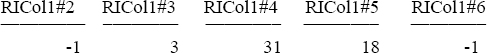
A regression line is a line of best fit, drawn through a set of points on a graph for X and Y coordinates. It uses the Y coordinate as the Dependent Variable and the X value as the Independent Variable.
Two regression lines always meet or intercept at the mean of the data points(x,y), where x=AVG(x) and y=AVG(y) and is not usually one of the original data points.
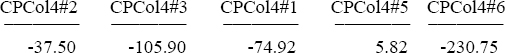
Another REGR_INTERCEPT Example so you can Compare
Stats_Table
SELECT
REGR_INTERCEPT(col4, col2) AS RICol4#2
,REGR_INTERCEPT(col4, col3) AS RICol4#3
,REGR_INTERCEPT(col4, col1) AS RICol4#1
,REGR_INTERCEPT(col4, col5) AS RICol4#5
,REGR_INTERCEPT(col4, col6) AS RICol4#6
FROM Stats_Table ;
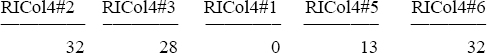
A regression line is a line of best fit, drawn through a set of points on a graph for X and Y coordinates. It uses the Y coordinate as the Dependent Variable and the X value as the Independent Variable.
Two regression lines always meet or intercept at the mean of the data points(x,y), where x=AVG(x) and y=AVG(y) and is not usually one of the original data points.
The REGR_SLOPE Function
SELECT REGR_SLOPE(col1, col2) AS RSCol1#2
FROM Stats_Table;
A regression line is a line of best fit, drawn through a set of points on a graph of X and Y coordinates. It uses the Y coordinate as the Dependent Variable and the X value as the Independent Variable.
The slope of the line is the angle at which it moves on the X and Y coordinates. The vertical slope is Y on X and the horizontal slope is X on Y.
Syntax for using REGR_SLOPE:
REGR_SLOPE(dependent-expression, independent-expression)
A REGR_SLOPE Example
Stats_Table
SELECT
REGR_SLOPE(col1, col2) AS RSCol1#2
,REGR_SLOPE(col1, col3) AS RSCol1#3
,REGR_SLOPE(col1, col4) AS RSCol1#4
,REGR_SLOPE(col1, col5) AS RSCol1#5
,REGR_SLOPE(col1, col6) AS RSCol1#6
FROM Stats_Table ;

A regression line is a line of best fit, drawn through a set of points on a graph of X and Y coordinates. It uses the Y coordinate as the Dependent Variable and the X value as the Independent Variable.
The slope of the line is the angle at which it moves on the X and Y coordinates. The vertical slope is Y on X and the horizontal slope is X on Y.
Another REGR_SLOPE Example so you can Compare
Stats_Table
SELECT
REGR_SLOPE(col4, col2) AS RSofCol1#2
,REGR_SLOPE(col4, col3) AS RSofCol1#3
,REGR_SLOPE(col4, col1) AS RSofCol1#4
,REGR_SLOPE(col4, col5) AS RSofCol1#5
,REGR_SLOPE(col4, col6) AS RSofCol1#6
FROM Stats_Table ;

A regression tine is a tine of best fit, drawn through a set of points on a graph of X and Y coordinates. It uses the Y coordinate as the Dependent Variable and the X value as the Independent Variable.
The slope of the tine is the angle at which it moves on the X and Y coordinates. The vertical slope is Y on X and the horizontal slope is X on Y.
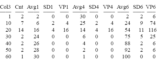
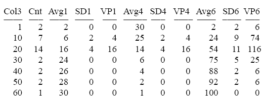
Using GROUP BY

SELECT col3
,count(*) AS Cnt
,avg(col1) AS Avg1
,stddev_pop(col1) AS SD1
,var_pop(col1) AS VP1
,avg(col4) AS Avg4
,stddev_pop(col4) AS SD4
,var_pop(col4) AS VP4
,avg(col6) AS Avg6
,stddev_pop(col6) AS SD6
,var_pop(col6) AS VP6
FROM Stats_Table
GROUP BY 1
ORDER BY 1;
No Having Clause Vs Use of HAVING
SELECT col3
,count(*) AS Cnt
,avg(col1) AS Avg1
,stddev_pop(col1) AS SD1
,var_pop(col1) AS VP1
,avg(col4) AS Avg4
,stddev_pop(col4) AS SD4
,var_pop(col4) AS VP4
,avg(col6) AS Avg6
,stddev_pop(col6) AS SD6
,var_pop(col6) AS VP6
FROM Stats_Table
GROUP BY 1
ORDER BY 1;
SELECT col3
,count(*) AS Cnt
,avg(col1) AS Avg1
,stddev_pop(col1) AS SD1
,var_pop(col1) AS VP1
FROM Stats_Table
GROUP BY 1
ORDER BY 1
HAVING Cnt > 2 and VP1 < 20;

The example (above right) uses HAVING to perform a compound comparison on both the count and the covariance