Chapter 7 – Aster Modeling Rules

“I know that you believe that you understand what you think I said, but I am not sure you realize that what you heard is not what I meant.”

-Sign on Pentagon office wall

Modeling Rules for Aster Data

Below are some excellent modeling rules for Aster Data:

1. Dimensionalize your schema.

2. Use Columnar techniques when appropriate.

3. Distribute your data by hash or replication with joins in mind.

4. Replicate frequently joined rows on Dimension Tables.

5. Use Logical partitioning on Fact tables when appropriate.

6. Make your Fact tables skinny.

7. Index your tables.

8. Consider denormalizing based on your environment.

Above are the eight rules for modeling Aster Data. These are designed around three principles which we will see on the next page

Three Principles that Govern the Modeling Rules

There are three principles for Aster Data modeling rules:

1. Do not move big data across the network. If you need to move big data, make it small first, and then move the smallest amount of data first.

2. Do not read irrelevant data. Design the data model so that the least amount of data is placed into memory for processing.

3. Process data only one time. Prepare your queries such that each computation is done never more than once.

Above are the eight rules for modeling Aster Data, but these are designed around three principles which are all about data movement, data access, and data processing.

Modeling Rule 1 – Dimensionalize your Model

A star schema model, also known as a Dimensional Model, is designed to take large amounts of legacy data, which has many columns and millions of rows, and to place the frequently read columns into skinny fact tables, and place the less frequently read columns into separate dimension tables. A fact table will have many rows and less columns, and a dimension table will have fewer rows and more columns.

A Dimensional Model is called a “Star Schema”

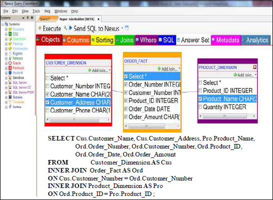
Nexus guides you to what tables join to what tables, and then as you click on the tables and columns you want on your report, Nexus builds the SQL for you.

To Read a Data Block, a vworker Moves the Block to Memory

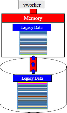
To read data, a vworker must transfer the entire data block from inside its disk to its dedicated memory. Even if the data has hundreds of columns and the query only needs to read a couple of the columns, the entire block must be transferred into memory.

A Dimensional Model Moves Less Mass into Memory

To read data, a vworker must transfer the entire data block from inside its disk to its dedicated memory. Why move data blocks with hundreds of columns just to query only a couple of columns? A Dimensional Model will move much less data.

Which Move From Disk to Memory Would You Choose?

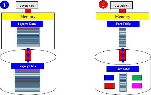
The name of the game is less movement and less mass from disk to memory. If the query only needs a few columns, then it does not make sense to move mass amounts of data into memory just to read a couple of the columns. That is why you use dimensions.

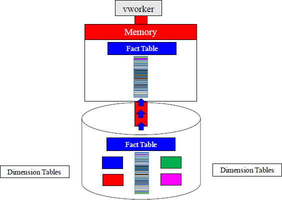
Vworkers transfer their Fact Table into Memory in Parallel

In the above diagram, the Fact Table has spread its rows via a hash so there are different rows on different vworkers. Each vworker transfers the rows of the fact table they are responsible for into memory, and parallel processing is at its best.

Modeling Rule 2 – Use Columnar

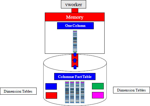
A Columnar Table breaks the table into separate blocks per column. If your query only needs one column (or a few), then why move data from disk to memory that you don’t need? A Columnar table is brilliant when the query can be satisfied with less columns.

Which Move From Disk to Memory Would You Choose?

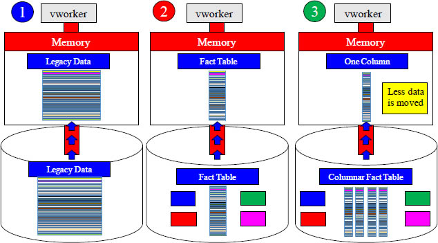
The name of the game is less movement and less mass from disk to memory. If the query only needs a single column, then it does not make sense to move more than one column into memory. Example 3 moves less data from disk into memory.

Let's Discuss Modeling and Joins at the Simplest Level

Notice all of the repeating information in blue.

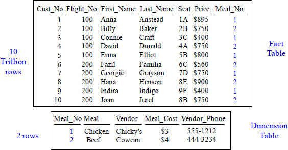
Now imagine that this table held 10 Trillion rows.

Turn the page and see how we modeled this data.

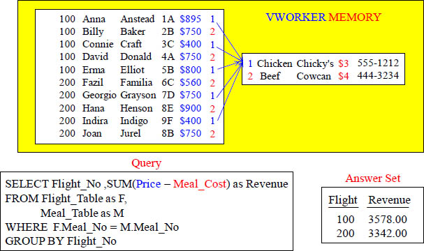
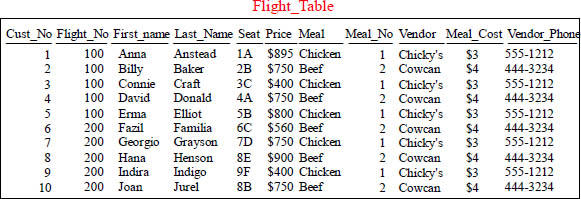
Above, we have a spreadsheet showing customers who took a flight. It also shows the meal they had. Notice that it has a bunch of repeating information about the meal and the meal vendor. Now imagine that this data was not just 10 rows, but 10 trillion rows. Data is modeled to save space and time. Watch how this information can be changed.

Let's Discuss Modeling and Joins at the Simplest Level

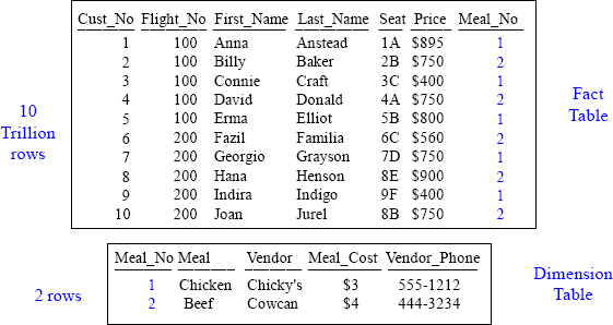
What is the price of Anna Anstead's meal vs. Billy Baker's meal?

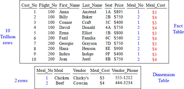
We have placed the redundant data into a separate table and we saved enormous space and time. Before, if we needed to update the meal price, we would have to update 10 trillion rows, but now we only have to update one or two rows. This is why we model. The 10 Trillion row fact table contains information about the flight and the dimension table contains information about the meal. We still have the same information, but it is now modeled. Anna's meal is $3 and Billy's is $4. You knew this because you did a join in your mind. Both tables contain Meal_No, so that is the join condition.

Let's Discuss Joins at the Simplest Level

Listen to me very carefully! Two rows can NOT be joined together unless they physically reside in the same memory of a vworker. The matching rows between the Flight_Table and the Meal_Table reside in the memory of this vworker.

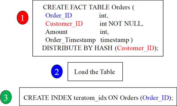
Modeling Rule 3 – Distribute your Tables Based on Joins

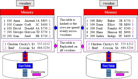
The Flight_Table is hashed by Cust_No, and so the 10 trillion rows are spread across many vworkers. The Flight Table is a Fact Table. To accomplish the Join rule where matching rows are on the same vworker, the Meal_Table is Replicated on all vworkers.

The Two Different Philosophies for Table Join Design

One table is Distributed by Hash, and the other is Distribute by Replication

Both tables Distribute by Hash on Customer_ID.

Both examples will have co-location of joins on the same vworker. Fact tables are always Distribute by Hash, but Dimension table can Distribute by Hash or Replication.

Facts are Hashed and most often the Dimension is Replicated

For two rows to be joined together, they must reside (physically) on the same vworker. That is why smaller tables are replicated. This guarantees a local join to the Fact table.

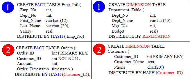
Fact and Dimension Tables can be Hashed by the same Key

Fact tables are large and usually distributed by hash. Dimension tables are usually small and often distributed by replication, but dimension tables can be distributed by hash. This is done to get vworker co-location. Above, you can see that both tables above where distributed by hash on the customer_id column. When these two tables are joined together where customer_id = customer_id, the matching rows are co-located.

Joining Two Tables with the same PK/FK Primary Index

The matching rows naturally distribute to the same vworker

CustNo is the join condition (PK/FK), so the matching customer numbers are on the same vworker. They were hashed there originally. Each customer has placed one order. Aster Data will have each vworker move their blocks into memory and perform a “Row Hash Join”. Those key words in the Explain tell you the join is taking place.

A Join With No Redistribution or Duplication

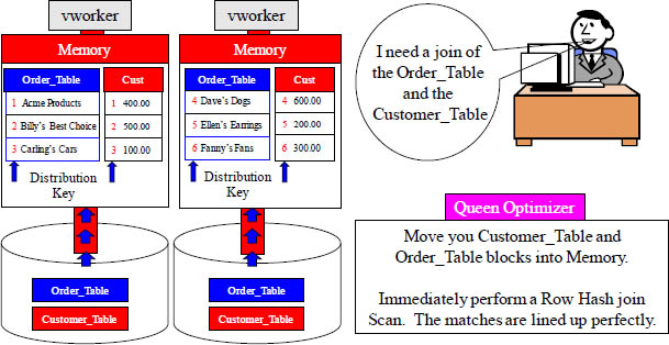
Both tables have the same Hash Key, and it is the join condition of CustNo. The matching rows are already on the same vworker because both tables joined on CustNo and their Distribution Key is on CustNo. Aster wants no unnecessary movement.

Aster Hates Joining Tables with a Different Distribution Key

The matching rows do NOT distribute to the same vworker.

CustNo is the join condition, but the matching customer numbers are on different vworkers. This is because the Order_Table is Distributed by Hash on Order_Number. Aster will redistribute the Order_Table by a Hash of CustNo so that the matching rows are on the same vworker. This is one of the things Aster hates to have to do.

Aster Hates to Redistribute by Hash to Join Tables

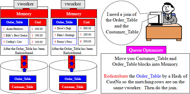
Both tables do NOT have the same Hash Key on the join condition of CustNo. The Order_Table has originally been hashed by OrderNo. To get the matching CustNo's on the same vworker, Aster will have to redistribute the Order_Table by CustNo.

Modeling Rule 4 – Replicate Dimension Tables

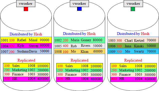
A Fact table will often join to multiple Dimension tables. For a join to take place, the matching rows must physically reside in the memory of the same vworker. Fact table are large and hashed to spread the rows equally among the vworkers with each vworker responsible for some of the rows.

The Dimension tables are replicated in their entirety and placed on each vworker, so the joining rows from fact to dimension are on the same vworker. Replicated means an exact copy of all the rows on every vworker.

Aster never wants to do a join unless the matching rows are on the same vworker. That is why, most of the time, they want the dimension tables replicated on every vworker.

Modeling Rule 5 – Partition Your Tables

The orders have been hashed equally across vworkers with each vworker responsible for orders assigned to them. There is no duplication or rows across vworkers. Then, to speed things up further, the vworkers partition their orders by month. Think of it like this: Instead of each vworker having one big yearly table, they have 12 smaller tables.

Modeling Rule 6 – Make Fact Tables Skinny

Notice all of the repeating information in blue.

This is not a skinny Fact table.

Now imagine that this table held 10 Trillion rows.

There would be enormous bulk on 10 Trillion rows.

Turn the page to see how we make this Fact table skinny.

Modeling Rule 6 – Make Fact Tables Skinny Example

Instead of having 10 Trillion rows with this extra information, we have cut it down to two rows. If we need all the information, we can perform a join.

We have placed the redundant data into a separate table, and we saved enormous space and time. Before, if we needed to update the meal price, we would have to update 10 trillion rows but now we only have to update one or two rows. This is why we model. The 10 Trillion row fact table contains information about the flight and the dimension table contains information about the meal. We still have the same information, but it is now modeled. The fact table will have the most rows so keeping it as skinny as possible is the best thing for performance.

Modeling Rule 7 – Index Your Tables

Define indexes on a table if the column is used in the WHERE clause of the SQL to find a single row or typically only a few rows. Indexes can also be very useful for speeding up a group-by clause and can even be useful in many joins. A secondary index can slow down the load process, so it is best to create the index after the table has been loaded. If you are maintaining a table with a great deal of inserts, updates, and deletes, then drop the index and re-create it after the maintenance is complete.

The B-Tree Index

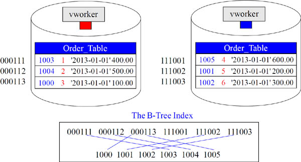
Indexes allow you to avoid a Full Table Scan. If the query has the indexed column in its WHERE clause and Aster estimates it will have to select less than 20% of the rows in the table, then Aster will choose the index scan rather than the Full Table Scan. A B-tree index is organized like an upside-down tree. The roots at the bottom level of the index holds the actual data values and then there are pointers to the corresponding rows. In a sense, it is like an index at the end of a book. Each value points to the page where each entry is present.

Which Columns Might You Create an Index?

Choose the best four secondary index choices from the above table.

Indexes allow you to avoid a Full Table Scan. If the query has the indexed column in its WHERE clause and Aster estimates it will have to select less than 20% of the rows in the table, then Aster will choose the index scan rather than the Full Table Scan. Which four secondary index choices would you most likely create for the Flight_Table? Turn the pages to see our opinion.

Answer - Which Columns Might You Create an Index?

CREATE INDEX choice1_idx ON Flight_Table (Cust_No);

CREATE INDEX choice2_idx ON Flight_Table (First_Name);

CREATE INDEX choice3_idx ON Flight_Table (Last_Name);

CREATE INDEX choice4_idx ON Flight_Table (First_Name, Last_Name);

Above are the best choices for indexing. Notice that we also created a multi-column index in example four.

Modeling Rule 8 – Denormalize based on Your Environment.

How might you denormalize these two tables?

If you are constantly joining two tables together and you are selecting only one column from one of the tables, you might want to denormalize and place that column is the other table especially if there are not a lot of deletes or updates. Then, instead of doing the join, you are only utilizing one table in most of the queries.

Modeling Rule 8 – Denormalize based on Your Environment.

How might you denormalize these two tables?

If you are constantly joining two tables together, and you are selecting only one column from one of the tables, you might want to denormalize and place that column is the other table especially if there are not a lot of deletes or updates. Then, instead of doing the join you, are only utilizing one table in most of the queries.