C H A P T E R 11
![]()
SQLite Internals and New Features
Our last chapter is a collection of topics devoted to the internals of SQLite. The material here is collected from topics raised by Richard Hipp, SQLite's founder, over the past year or so. Importantly, we'll highlight one of the biggest changes to happen to SQLite in recent versions: the introduction of the Write-Ahead Log model. We'll also briefly explore how the pager and B-trees work and go into a little more detail on the underpinnings of data types, affinity, and the SQLite approach to typing.
This isn't an exhaustive description of the inner workings of SQLite, because that's covered very well on the SQLite web site, and the healthy rate of change for SQLite releases means that a book isn't always the best place to track things such as known commands in the VDBE, optimization models, and so on. We hope you enjoy these topics, and we encourage you to read more to further your understanding of the beauty and elegance of SQLite's design.
The B-Tree and Pager Modules
The B-tree provides SQLite's VDBE with O(logN) lookup, insert, and delete as well as O(1) bidirectional traversal of records. It is self-balancing and automatically manages both defragmentation and space reclamation. The B-tree itself has no notion of reading or writing to disk. It concerns itself only with the relationship between pages. The B-tree notifies the pager when it needs a page and also notifies it when it is about to modify a page. When modifying a page, the pager ensures that the original page is first copied out to the journal file if the traditional rollback journal is in use. Similarly, the B-tree notifies the pager when it is done writing, and the pager determines what needs to be done based on the transaction state.
Database File Format
All pages in a database are numbered sequentially, beginning with 1. A database is composed of multiple B-trees—one B-tree for each table and index (B+trees are used for tables; B-trees are used for indexes). Each table or index in a database has a root page that defines the location of its first page. The root pages for all indexes and tables are stored in the sqlite_master table.
The first page in the database—Page 1—is special. The first 100 bytes of Page 1 contain a special header (the file header) that describes the database file. It includes such information as the library version, schema version, page size, encoding, whether autovacuum is enabled—all of the permanent database settings you configure when creating a database along with any other parameters that have been set by various pragmas. The exact contents of the header are documented in btree.c and at http://www.sqlite.org/fileformat2.html. Page 1 is also the root page of the sqlite_master table.
Page Reuse and Vacuum
SQLite recycles pages using a free list. That is, when all the records are deleted out of a page, the page is placed on a list reserved for reuse. When new information is later added, nearby pages are first selected before any new pages are created (expanding the database file). Running a VACUUM command purges the free list and thereby shrinks the database. In actuality, it rebuilds the database in a new file so that all in-use pages are copied over, while free-list pages are not. The end result is a new, compacted database. When autovacuum is enabled in a database, SQLite doesn't use a free list and automatically shrinks the database upon each commit.
B-Tree Records
Pages in a B-tree consist of B-tree records, also called payloads. They are not database records in the sense you might think—formatted with the columns in a table. They are more primitive than that. A B-tree record, or payload, has only two fields: a key field and a data field. The key field is the rowid value or primary key value that is present for every table in the database. The data field, from the B-tree perspective, is an amorphous blob that can contain anything. Ultimately, the database records are stored inside the data fields. The B-tree's job is order and navigation, and it primarily needs only the key field to do its work (however, there is one exception in B+trees, which is addressed next). Furthermore, payloads are variable size, as are their internal key and data fields. On average, each page usually holds multiple payloads; however, it is possible for a payload to span multiple pages if it is too large to fit on one page (for example, records containing blobs).
B+Trees
B-tree records are stored in key order. All keys must be unique within a single B-tree (this is automatically guaranteed because the keys correspond to the rowid primary key, and SQLite takes care of that field for you). Tables use B+trees, which do not contain table data (database records) in the internal pages. Figure 11-1 shows an example B+tree representation of a table.
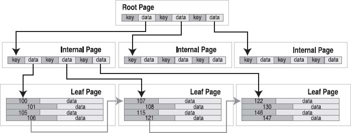
Figure 11-1. B+tree organization (tables)
The root page and internal pages in B+trees are all about navigation. The data fields in these pages are all pointers to the pages below them—they contain keys only. All database records are stored on the leaf pages. On the leaf level, records and pages are arranged in key order so it is possible for B-tree cursors to traverse records (horizontally), both forward and backward, using only the leaf pages. This is what makes traversal possible in O(1) time.
Records and Fields
The database records in the data fields of the leaf pages are managed by the VDBE. The database record is stored in binary form using a specialized record format that describes all the fields in the record. The record format consists of a continuous stream of bytes organized into a logical header and a data segment. The header segment includes the header size (represented as a variable-sized 64-bit integer value) and an array of types (also variable 64-bit integers), which describe each field stored in the data segment, as shown in Figure 11-2. Variable 64-bit integers are implemented using a Huffman code.
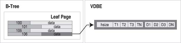
Figure 11-2. Record structure
The number of type entries corresponds to the number of fields in the record. Furthermore, each index in the type array corresponds to the same index in the field array. A type entry specifies the data type and size of its corresponding field value. Table 11-1 lists the possible types and their meanings.
| Type Value | Meaning | Length of Data |
| 0 | NULL |
0 |
| N in 1..4 | Signed integer | N |
| 5 Signed | integer | 6 |
| 6 Signed | integer | 8 |
| 7 IEEE | float | 8 |
| 8 | Integer constant 0 | 0 |
| 9 | Integer constant 1 | 0 |
| 10-11 | Reserved for future use | N/A |
| N>12 and even | blob |
(N-12)/2 |
| N>13 and odd | text |
(N-13)/2 |
For example, take the first record in the episodes table:
sqlite> SELECT * FROM episodes ORDER BY id LIMIT 1;

id   season  name

---  ------  --------------------

0    1       Good News Bad News
Figure 11-3 shows the internal record format for this record.
Figure 11-3. First record in the episodes table
The header is 4 bytes long. The header size reflects this and itself is encoded as a single byte. The first type, corresponding to the id field, is a 1-byte signed integer. The second type, corresponding to the season field, is as well. The name type entry is an odd number, meaning it is a text value. Its size is therefore given by (49-13)/2=17 bytes. With this information, the VDBE can parse the data segment of the record and extract the individual fields.
Hierarchical Data Organization
Basically, each module in the stack deals with a specific unit of data. From the bottom up, data becomes more refined and more specific. From the top down, it becomes more aggregated and amorphous. Specifically, the C API deals in field values, the VDBE deals in records, the B-tree deals in keys and data, the pager deals in pages, and the OS interface deals in binary data and raw storage, as illustrated in Figure 11-4.
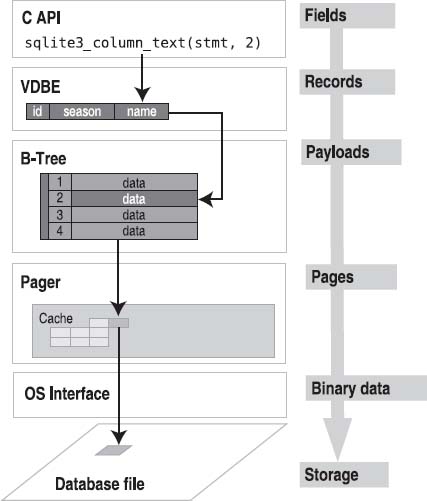
Figure 11-4. Modules and their associated data
Each module takes part in managing its own specific portion of the data in the database and relies on the layer below it to supply it with a cruder form from which to extract its respective pieces.
Overflow Pages
As mentioned earlier, payloads and their contents can have variable sizes. However, pages are fixed in size. Therefore, there is always the possibility that a given payload could be too large to fit in a single page. When this happens, the excess payload is spilled out onto a linked list of overflow pages. From this point on, the payload takes on the form of a linked list of sorts, as shown in Figure 11-5.
The fourth payload in the figure is too large to fit on the page. As a result, the B-tree module creates an overflow page to accommodate. It turns out that one page won't suffice, so it links a second. This is essentially the way binary large objects are handled. One thing to keep in mind when you are using really large blobs is that they are ultimately being stored as a linked list of pages. If the blob is large enough, this can become inefficient, in which case you might consider dedicating an external file for the blob and keeping this file name in the record instead.
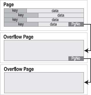
Figure 11-5. Overflow pages
The B-Tree API
The B-tree module has its own API, which is separate from the C API. We'll explore it here for completeness, but it's not really meant as a general-purpose B-tree API. You'll see it is heavily tailored to the needs of SQLite, so it's not really suitable for you to just pick up and drop into some other project. That said, understanding it in depth will allow you to appreciate even more of SQLite's internals. An added benefit of SQLite's B-tree module is that it includes native support for transactions. Everything you know about the transactions, locks, and journal files are handled by the pager, which serves the B-tree module. The API can be grouped into functions according to general purpose.
Access and Transaction Functions
Database and transaction routines include the following:
sqlite3BtreeOpen: Opens a new database file. Returns a B-tree object.sqlite3BtreeClose: Closes a database.sqlite3BtreeBeginTrans: Starts a new transaction.sqlite3BtreeCommit: Commits the current transaction.sqlite3BtreeRollback: Rolls back the current transaction.sqlite3BtreeBeginStmt: Starts a statement transaction.sqlite3BtreeCommitStmt: Commits a statement transaction.sqlite3BtreeRollbackStmtsqlite3BtreeRollbackStmt: Rolls back a statement transaction.
Table Functions
Table management routines include the following:
sqlite3BtreeCreateTable: Creates a new, empty B-tree in a database file. Flags in the argument determine whether to use a table format (B+tree) or index format (B-tree).sqlite3BtreeDropTable: Destroys a B-tree in a database file.sqlite3BtreeClearTable: Removes all data from a B-tree but keeps the B-tree intact.
Cursor Functions
Cursor functions include the following:
sqlite3BtreeCursor: Creates a new cursor pointing to a particular B-tree. Cursors can be either a read cursor or a write cursor. Read and write cursors may not exist in the same B-tree at the same time.sqlite3BtreeCloseCursor: Closes the B-tree cursor.sqlite3BtreeFirst: Moves the cursor to the first element in a B-tree.sqlite3BtreeLast: Moves the cursor to the last element in a B-tree.sqlite3BtreeNext: Moves the cursor to the next element after the one it is currently pointing to.sqlite3BtreePrevious: Moves the cursor to the previous element before the one it is currently pointing to.sqlite3BtreeMoveto: Moves the cursor to an element that matches the key value passed in as a parameter. If there is no match, leaves the cursor pointing to an element that would be on either side of the matching element, had it existed.
Record Functions
Key and record functions include the following:
sqlite3BtreeDelete: Deletes the record to which the cursor is pointingsqlite3BtreeInsert: Inserts a new element in the appropriate place of the B-treesqlite3BtreeKeySize: Returns the number of bytes in the key of the record to which the cursor is pointingsqlite3BtreeKey: Returns the key of the record to which the cursor is currently pointingsqlite3BtreeDataSize: Returns the number of bytes in the data record to which the cursor is currently pointingsqlite3BtreeData: Returns the data in the record to which the cursor is currently pointing
Configuration Functions
Functions to set various parameters include the following:
sqlite3BtreeSetCacheSize: Controls the page cache size as well as the synchronous writes (as defined in thesynchronouspragma).sqlite3BtreeSetSafetyLevel: Changes the way data is synced to disk in order to increase or decrease how well the database resists damage because of OS crashes and power failures. Level 1 is the same as asynchronous (nosyncs()occur, and there is a high probability of damage). This is the equivalent to pragmasynchronous=OFF. Level 2 is the default. There is a very low but nonzero probability of damage. This is the equivalent to pragmasynchronous=NORMAL. Level 3 reduces the probability of damage to near zero but with a write performance reduction. This is the equivalent to pragmasynchronous=FULL.sqlite3BtreeSetPageSize: Sets the database page size.sqlite3BtreeGetPageSize: Returns the database page size.sqlite3BtreeSetAutoVacuum: Sets the autovacuum property of the database.sqlite3BtreeGetAutoVacuum: Returns whether the database uses autovacuum.sqlite3BtreeSetBusyHandler: Sets the busy handler.
There are more functions, all of which are very well documented in btree.h and btree.c, but those listed here give you some idea of the parts of the API that are implemented in the B-tree layer, as well as what this layer can do in its own right.
Manifest Typing, Storage Classes, and Affinity
You'll remember from Chapter 4 our discussion on storage classes in SQLite and how its underlying data typing (or domains) offers a rather more flexible approach to the notion of data types that you find in other systems or databases. It's worth exploring the mechanisms that underpin storage classes further, including SQLite's approach to manifest typing and type affinity.
Manifest Typing
SQLite uses manifest typing. If you do a little research, you will find that the term manifest typing is subject to multiple interpretations. In programming languages, manifest typing refers to how the type of a variable or value is defined and/or determined. There are two main interpretations:
- Manifest typing means that a variable's type must be explicitly declared in the code. By this definition, languages such as C/C++, Pascal, and Java would be said to use manifest typing. Dynamically typed languages such as Perl, Python, and Ruby, on the other hand, are the direct opposite because they do not require that a variable's type be declared.
- Manifest typing means that variables don't have types at all. Rather, only values have types. This seems to be in line with dynamically typed languages. Basically, a variable can hold any value, and the type of that variable at any point in time is determined by its value at that moment. Thus, if you set variable
x=1, thenxat that moment is of typeinteger. If you then setx='JujyFruit', it is then of typetext. That is, if it looks like anintegerand it acts like aninteger, it is aninteger.
For the sake of brevity, we will refer to the first interpretation as MT 1 and the second as MT 2. At first glance, it may not be readily apparent as to which interpretation best fits SQLite. For example, consider the following table:
create table foo( x integer,

                  y text,

                  z real );
Say we now insert a record into this table as follows:
insert into foo values ('1', '1', '1'),
When SQLite creates the record, what type is stored internally for x, y, and z? The answer is integer, text, and real. Then it seems that SQLite uses MT 1: variables have declared types. But wait a second; column types in SQLite are optional, so we could have just as easily defined foo as follows:
create table foo(x, y, z);
Now let's do the same insert:
insert into foo values ('1', '1', '1'),
What type are x, y, and z now? The answer: text, text, and text. Well, maybe SQLite is just setting columns to text by default. If you think that, then consider the following insert statement on the same table:
INSERT INTO FOO VALUES (1, 1.0, x'10'),
What are x, y, and z in this row? integer, real, and blob. This looks like MT 2, where the value itself determines its type.
So, which one is it? The short answer is neither and both. The long answer is a little more involved. With respect to MT 1, SQLite lets you declare columns to have types if you want. This looks and feels like what other databases do. But you don't have to, thereby violating the MT1 interpretation as well. This is because in all situations SQLite can take any value and infer a type from it. It doesn't need the type declared in the column to help it out. With respect to MT 2, SQLite allows the type of the value to “influence” (maybe not completely determine) the type that gets stored in the column. But you can still declare the column with a type, and that type will exert some influence, thereby violating this interpretation as well—that types come from values only. What we really have here is the MT 3—the SQLite interpretation. It borrows from both MT 1 and MT 2.
But interestingly enough, manifest typing does not address the whole issue with respect to types. It seems to be concerned with only declaring and resolving types. What about type checking? That is, if you declare a column to be type integer, what exactly does that mean?
First let's consider what most other relational databases do. They enforce strict type checking as a standard part of standard domain integrity. First you declare a column's type. Then only values of that type can go in it. End of story. You can use additional domain constraints if you want, but under no conditions can you ever insert values of other types. Consider the following example with Oracle:
SQL> create table domain(x int, y varchar(2));

Table created.


SQL> insert into domain values ('pi', 3.14);

insert into domain values ('pi', 3.14)

                         *

ERROR at line 1:

ORA-01722: invalid number
The value 'pi' is not an integer value. And column x was declared to be of type int. We don't even get to hear about the error in column y because the whole insert is aborted because of the integrity violation on x. When I try this in SQLite, we said one thing and did another, and SQLite didn't stop me:
sqlite> create table domain (x int, y varchar(2));

sqlite> INSERT INTO DOMAIN VALUES ('pi', 3.14);

sqlite> select * from domain;


x     y

----  -----

pi    3.14
SQLite's domain integrity does not include strict type checking. So, what is going on? Does a column's declared type count for anything? Yes. Then how is it used? It is all done with something called type affinity.
In short, SQLite's manifest typing states that columns can have types and that types can be inferred from values. Type affinity addresses how these two things relate to one another. Type affinity is a delicate balancing act that sits between strict typing and dynamic typing.
Type Affinity
In SQLite, columns don't have types or domains. Although a column can have a declared type, internally it has only a type affinity. Declared type and type affinity are two different things. Type affinity determines the storage class SQLite uses to store values within a column. The actual storage class a column uses to store a given value is a function of both the value's storage class and the column's affinity. Before getting into how this is done, however, let's first talk about how a column gets its affinity.
Column Types and Affinities
To begin with, every column has an affinity. There are four different kinds: numeric, integer, text, and none. A column's affinity is determined directly from its declared type (or lack thereof). Therefore, when you declare a column in a table, the type you choose to declare it will ultimately determine that column's affinity. SQLite assigns a column's affinity according to the following rules:
- By default, a column's default affinity is
numeric. That is, if a column is notinteger,text, ornone, then it is automatically assignednumericaffinity. - If a column's declared type contains the string
'int'(in uppercase or lowercase), then the column is assignedintegeraffinity. - If a column's declared type contains any of the strings
'char','clob', or'text'(in uppercase or lowercase), then that column is assignedtextaffinity. Notice that 'varchar'contains the string'char'and thus will confertextaffinity. - If a column's declared type contains the string
'blob'(in uppercase or lowercase), or if it has no declared type, then it is assignednoneaffinity.
![]() Note Pay attention to defaults. For instance,
Note Pay attention to defaults. For instance, floatingpoint has affinity integer. If you don't declare a column's type, then its affinity will be none, in which case all values will be stored using their given storage class (or inferred from their representation). If you are not sure what you want to put in a column or want to leave it open to change, this is the best affinity to use. However, be careful of the scenario where you declare a type that does not match any of the rules for none, text, or integer. Although you might intuitively think the default should be none, it is actually numeric. For example, if you declare a column of type JUJYFRUIT, it will not have affinity none just because SQLite doesn't recognize it. Rather, it will have affinity numeric. (Interestingly, the scenario also happens when you declare a column's type to be numeric for the same reason.) Rather than using an unrecognized type that ends up as numeric, you may prefer to leave the column's declared type out altogether, which will ensure it has affinity none.
Affinities and Storage
Each affinity influences how values are stored in its associated column. The rules governing storage are as follows:
- A
numericcolumn may contain all five storage classes. Anumericcolumn has a bias toward numeric storage classes (integerandreal). When atextvalue is inserted into anumericcolumn, it will attempt to convert it to anintegerstorage class. If this fails, it will attempt to convert it to arealstorage class. Failing that, it stores the value using thetextstorage class. - An
integercolumn tries to be as much like anumericcolumn as it can. Anintegercolumn will store arealvalue asreal. However, if arealvalue has no fractional component, then it will be stored using anintegerstorage class.integercolumn will try to store atextvalue asrealif possible. If that fails, they try to store it asinteger. Failing that,textvalues are stored asTEXT. - A
textcolumn will convert allintegerorrealvalues totext. - A
nonecolumn does not attempt to convert any values. All values are stored using their given storage class. - No column will ever try to convert
nullorblobvalues—regardless of affinity.nullandblobvalues are always stored as is in every column.
These rules may initially appear somewhat complex, but their overall design goal is simple: to make it possible for SQLite to mimic other relational databases if you need it to do so. That is, if you treat columns like a traditional database, type affinity rules will store values in the way you expect. If you declare a column of type integer and put integers into it, they will be stored as integer. If you declare a column to be of type text, char, or varchar and put integers into it, they will be stored as text. However, if you don't follow these conventions, SQLite will still find a way to store the value.
Affinities in Action
Let's look at a few examples to get the hang of how affinity works. Consider the following:
sqlite> create table domain(i int, n numeric, t text, b blob);

sqlite> insert into domain values (3.142,3.142,3.142,3.142);

sqlite> insert into domain values ('3.142','3.142','3.142','3.142'),

sqlite> insert into domain values (3142,3142,3142,3142);

sqlite> insert into domain values (x'3142',x'3142',x'3142',x'3142'),

sqlite> insert into domain values (null,null,null,null);

sqlite> select rowid,typeof(i),typeof(n),typeof(t),typeof(b) from domain;


rowid       typeof(i)   typeof(n)   typeof(t)   typeof(b)

----------  ----------  ----------  ----------  ----------

1           real        real        text        real

2           real        real        text        text

3           integer     integer     text        integer

4           blob        blob        blob        blob

5           null        null        null        null
The first insert inserts a real value. You can see this both by the format in the insert statement and by the resulting type shown in the typeof(b) column returned in the select statement. Remember that blob columns have storage class none, which does not attempt to convert the storage class of the input value, so column b uses the same storage class that was defined in the insert statement. Column i keeps the numeric storage class, because it tries to be numeric when it can. Column n doesn't have to convert anything. Column t converts it to text. Column b stores it exactly as given in the context. In each subsequent insert, you can see how the conversion rules are applied in each varying case.
The following SQL illustrates storage class sort order and interclass comparison (which are governed by the same set of rules):
sqlite> select rowid, b, typeof(b) from domain order by b;


rowid  b       typeof(b)

-----  ------  ---------

5      NULL    null

1      3.142   real

3      3142    integer

2      3.142   text

4      1B      blob
Here, you see that nulls sort first, followed by integers and reals, followed by texts and then blobs. The following SQL shows how these values compare with the integer 1,000. The integer and real values in b are less than 1,000 because they are numerically compared, while text and blob are greater than 1,000 because they are in a higher storage class.
sqlite> select rowid, b, typeof(b), b<1000 from domain order by b;


rowid  b      typeof(b)  b<1000

-----  -----  --------  ----------

5      NULL   null      NULL

1      3.142  real      1

3      3142   integer   1

2      3.142  text      0

4      1B     blob      0
The primary difference between type affinity and strict typing is that type affinity will never issue a constraint violation for incompatible data types. SQLite will always find a data type to put any value into any column. The only question is what type it will use to do so. The only role of a column's declared type in SQLite is simply to determine its affinity. Ultimately, it is the column's affinity that has any bearing on how values are stored inside of it. However, SQLite does provide facilities for ensuring that a column may only accept a given type or range of types. You do this using check constraints, explained in the sidebar “Makeshift Strict Typing” later in this section.
Storage Classes and Type Conversions
Another thing to note about storage classes is that they can sometimes influence how values are compared as well. Specifically, SQLite will sometimes convert values between numeric storage classes (integer and real) and text before comparing them. For binary comparisons, it uses the following rules:
- When a column value is compared to the result of an expression, the affinity of the column is applied to the result of the expression before the comparison takes place.
- When two column values are compared, if one column has
integerornumericaffinity and the other doesn't, thennumericaffinity is applied totextvalues in the non-numericcolumn. - When two expressions are compared, SQLite does not make any conversions. The results are compared as is. If the expressions are of like storage classes, then the comparison function associated with that storage class is used to compare values. Otherwise, they are compared on the basis of their storage class.
Note that the term expression here refers to any scalar expression or literal other than a column value. To illustrate the first rule, consider the following:
sqlite> select rowid,b,typeof(i),i>'2.9' from domain order by b;


rowid  b      typeof(i  i>'2.9'

-----  -----  --------  ------------

5      NULL   null      NULL

1      3.142  real      1

3      3142   integer   1

2      3.142  real      1

4      1B     blob      1
The expression '2.9', while being text, is converted to integer before the comparison. So, the column interprets the value in light of what it is. What if '2.is a non-numeric string? Then SQLite falls back to comparing storage class, in which integer and numeric types are always less than text:
sqlite> select rowid,b,typeof(i),i>'text' from domain order by b;


rowid  b      typeof(i  i>'text'

-----  -----  --------  ------------

5      NULL   null      NULL

1      3.14   real      0

3      314    integer   0

2      3.14   real      0

4      1B     blob      1
The second rule simply states that when comparing a numeric and non-numeric column, where possible SQLite will try to convert the non-numeric column to numeric format:
sqlite> create table rule2(a int, b text);

sqlite> insert into rule2 values(2,'1'),

sqlite> insert into rule2 values(2,'text'),

sqlite> select a, typeof(a),b,typeof(b), a>b from rule2;


a           typeof(a)   b           typeof(b)   a>b

----------  ----------  ----------  ----------  ----------

2           integer     1           text        1

2           integer     text        text        0
Column a is an integer, and b is text. When evaluating the expression a>b, SQLite tries to coerce b to integer where it can. In the first row, b is '1', which can be coerced to integer. SQLite makes the conversion and compares integers. In the second row, b is 'text' and can't be converted. SQLite then compares storage classes integer and text.
The third rule just reiterates that storage classes established by context are compared at face value. If what looks like a text type is compared with what looks like an integer type, then text is greater.
Additionally, you can manually convert the storage type of a column or an expression using the cast() function. Consider the following example:
sqlite> select typeof(3.14), typeof(cast(3.14 as text));


typeof(3.14)  typeof(cast(3.14 as text))

------------  --------------------------

real          text
MAKESHIFT STRICT TYPING
Write Ahead Logging
With the release of SQLite 3.7.0, a new optional model for managing atomic transactions was introduced: the Write Ahead Log. The Write Ahead Log (WAL) is not new to the wider database technology world, but it's inclusion in SQLite is amazing for two reasons. First, this further enhances the sophistication and robustness of SQLite and the databases you use. Second, it's astounding that such a great feature has been included in SQLite and yet the code and resulting binaries are still so compact and concise.
How WAL Works
In the traditional mode of operation, SQLite uses the rollback journal to capture the prechange data from your SQL statements and then makes changes to the database file (we'll avoid discussing the various caching and file system layers here, because they apply regardless of model). When the WAL is used, the arrangement is reversed. Instead of writing the original, prechanged data to the rollback journal, using WAL leaves the original data untouched in the database file. The WAL file is used to record the changes to the data that occur for a given transaction. A commit action changes to being a special record written to the WAL to indicate the preceding changes are in fact complete and to be honored from an ACID perspective.
This change in roles between database file and log file immediately alters the performance dynamics of transactions. Instead of contending over the same pages in the database file, multiple transactions can simultaneously record their data changes in the WAL and can continue reading the unaltered data from the database file.
Checkpoints
The first question that most people think of when confronted with WAL technologies is usually “But when does the data ultimately get written to the database?” We're glad you asked. Obviously, a never-ending stream of changes being written to a constantly growing WAL file wouldn't scale or withstand the vagaries of file system failures. The WAL uses a checkpoint function to write changes back to the database. This process happens automatically, so the developer need not concern themselves with managing the checkpointing and write-back to the database. By default, the WAL invokes a checkpoint when the WAL file hits 1,000 pages of changes. This can be modified to suit different operating scenarios.
Concurrency
Because changes now write to the WAL file, rather than the database file, you might be wondering how this affects SQLite concurrency. The good news is the answer “overwhelmingly for the better!”
New readers accessing data from the WAL-enabled database initiate a lookup in the WAL file to determine the last commit record. This point becomes their end marker for read-only consistency, such that they will not consider new writes beyond this point in the file. This is how the read becomes a consistent read—it simply takes no notice of anything after the commit considered its end marker. Each reader assess is independent, so it's possible to have multiple threads each with a different notion of their own individual end mark within the WAL file.
To access a page of data, the reader uses a wal-index structure to scan the WAL file to find out whether the page exists with changes and uses the latest version if found. If the page isn't present in the WAL file, it means it hasn't been altered since the last checkpoint, and the reader accesses the page from the database file.
The wal-index structure is implemented in shared memory, meaning that all threads and processes must have access to the same memory space. That is, your programs must all execute on the same machine in order to access a WAL-enabled database or, more accurately, to use the wal-index. This is the feature that rules out operation across network file systems like NFS.
As for writers, thanks to the sequential nature of the WAL file, they simply append changes to the end. Note, however, that this means they must take it in turn appending their changes, so writers can still block writers.
Activation and Configuration WAL
SQLite will still default to the rollback journal method until you decide to switch your database to use the WAL. Unlike other PRAGMA settings, turning on the WAL is a persistent database-level change. This means you can turn on WAL in one program or from the SQLite command shell, and all other programs will then be using the database in WAL mode. This is very handy because it means you don't have to alter your applications to turn on WAL.
The setting PRAGMA journal_mode=WAL is the command necessary to activate WAL. A call to this pragma will return as a string the final journal mode for the database.
SQLite version 3.7.3

Enter ".help" for instructions

Enter SQL statements terminated with a ";"

sqlite> PRAGMA journal_mode=WAL;

wal
If the change to WAL is successful, the string wal is returned, as shown. If for some reason this fails, such as the underlying host not supporting the necessary shared memory requirements, the journal mode will be unchanged. For instance, on a default database, this means the command will return the string delete, meaning the rollback journal is still active.
As well as the journal_mode PRAGMA, several API options and related PRAGMAs are supported to control WAL and checkpoint behavior.
sqlite3_wal_checkpoint(): Forces a checkpoint (also available aswal_checkpoint PRAGMA)sqlite3_wal_autocheckpoint(): Alters autocheckpoint page threshold (wal_autocheckpoint PRAGMA)sqlite3_wal_hook(): Registers a callback to be invoked when a program commits to the WAL.
With these options, it's possible to fine-tune WAL and checkpoint behavior to suit even the most unusual of applications.
WAL Advantages and Disadvantages
Naturally, a change such as WAL brings with it its own advantages and disadvantages. We think that the advantages are significant, but it's best to be aware of impact so you can form your own judgment.
Moving to WAL has the following advantages:
- Readers do not block writers, and writers do not block readers. This is the “gold standard” in concurrency management.
- WAL is flat-out faster in most operating scenarios, when compared to rollback journaling.
- Disk I/O becomes more predictable and induces fewer
fsync()system calls. Because all WAL writes are to a linearly written log file, much of the I/O becomes sequential and can be planned accordingly.
To balance the equation, here are some of the notable disadvantages of WAL:
- All processing is bound to a single host. That is, you cannot use WAL over a networked file system like NFS.
- Using WAL introduces two additional semipersistent files,
<yourdb>-waland<yourdb>-shm, for the WAL and related shared memory requirements. This can be unappealing for those using SQLite databases as an application file format. This also affects read-only environments, because the–shmfile must be writable, and/or the directory in which the database exists. - WAL performance will degrade for very large (approaching gigabyte) transactions. Although WAL is a high-performance option, very large or very long-running transactions introduce additional overhead.
A number of other edge cases are worth investigating if you are thinking of using SQLite with WAL-enabled databases in unusual environments. You can review more details about these at www.sqlite.org/wal.html.
Operational Issues with WAL-Enabled SQLite Databases
There are a few operational considerations when working with WAL-enabled SQLite databases. These are primarily performance and recovery related.
Performance
We noted earlier that enabling WAL usually translates to better performance. Under our disadvantages, we outlined that for very large changes in data, or very long-running transactions, a slight drop in performance might result. Here's the background on how this can happen and what to do.
With WAL enabled, you implicitly gain a performance advantage over rollback journaling because only one write is required to commit a transaction, instead of two (one to the database and rollback journal). However, until a checkpoint occurs that frees space in the WAL file, the file itself must keep growing as more and more changes are recorded. Normally this isn't an issue: someone will be the lucky committer who pushes WAL through the 1,000-page threshold for a checkpoint, and the WAL will clear, and the cycle will continue. But the checkpoint completes its work if it finds an end-point marker for any currently active reader. That means a very long-running transaction or read activity can keep the checkpoint from making progress, even on subsequent attempts. This in turn means the WAL file keeps growing in size, with commensurately longer seek times for new readers to find pages.
Another performance consideration is how much work is triggered when a transaction hits the checkpoint threshold. You may find that the variable nature of lots of very fast transactions and then one slightly longer one that must perform the checkpoint work for its predecessors unattractive in some scenarios.
For both of these performance hypotheticals, you are essentially weighing up read and write performance. Our recommended approach is to first remember that you can't have the best of both, so some compromise will be needed, and then if necessary use the sqlite3_wal_checkpoint() and sqlite3_wal_autocheckpoint() tools to balance the load and find a happy equilibrium.
Recovery
Versions of SQLite prior to 3.7.0 have no knowledge of WAL, nor the methods used for recovering WAL-based databases. To prevent older versions trampling all over a WAL-enabled SQLite database during crash recovery, the database file format number was bumped up from 1 to 2. When an older version of SQLite attempts to recover a database with this change, it realizes it is not a “valid” SQLite database and will report an error similar to the following.
file is encrypted or is not a database
Don't panic! Your database is fine, but the version of SQLite will need to be upgraded in order to work with it. Alternatively, you can change back to the rollback journal.
PRAGMA journal_mode=DELETE;
This resets the database file format number to 1.
Summary
That concludes our journey through SQLite, not only in this chapter but the book as well. We hope you have enjoyed it. As you saw in Chapter 1, SQLite is more than merely a free database. It is a well-written software library with a wide range of applications. It is a database, a utility, and a helpful programming tool.
What you have seen in this chapter barely scratches the surface of the internals, but it should give you a better idea about how things work nonetheless. And it also gives you an appreciation for how elegantly SQLite approaches a very complex problem. You know firsthand how big SQL is, and you've seen the complexity of the models behind it. Yet SQLite is a small library and manages to put many of these concepts to work in a small amount of code and excels!