
Chapter 14
Stateless Application Patterns
THE AWS CERTIFIED DEVELOPER – ASSOCIATE EXAM TOPICS COVERED IN THIS CHAPTER INCLUDE, BUT ARE NOT LIMITED TO, THE FOLLOWING:
- Domain 1: Deployment
 1.4 Deploy serverless applications.
- Domain 2: Security
- 2.1 Make authenticated calls to AWS services.
- 2.2 Implement encryption using AWS services.
- 2.3 Implement application authentication and authorization.
- Domain 3: Development with AWS Services
- 3.2 Translate functional requirements into application design.
- 3.3 Implement application design into application code.
- 3.4 Write code that interacts with AWS services by using APIs, SDKs, and AWS CLI.

Introduction to the Stateless Application Pattern
In previous chapters, you were introduced to compute, networking, databases, and storage on the AWS Cloud. This chapter covers the fully managed services that you use to build stateless applications on AWS. Scalability is an important consideration when you create and deploy applications that are highly available, and stateless applications are easier to scale.
When users or services interact with an application, they often perform a sequence of interactions that form a session. A stateless application is one that requires no knowledge of previous interactions and stores no session information. Given the same input, an application can provide the same response to any user.
A stateless application can scale horizontally because requests can be serviced by any of the available compute resources, such as Amazon Elastic Compute Cloud (Amazon EC2) instances or AWS Lambda functions. With no session data sharing, you can add more compute resources as necessary. When that compute capacity is no longer needed, you can safely terminate any individual resource. Those resources do not need to be aware of the presence of their peers, and they only need a way to share the workload among them.
This chapter discusses the AWS services that provide a mechanism for persisting state outside of the application: Amazon DynamoDB, Amazon Simple Storage Service (Amazon S3), Amazon ElastiCache, and Amazon Elastic File System (Amazon EFS).
Amazon DynamoDB
Amazon DynamoDB is a fast and flexible NoSQL database service that applications use that require consistent, single-digit millisecond latency at any scale. A fully managed NoSQL database supports both document and key-value store models. DynamoDB is ideal for mobile, web, gaming, ad tech, and Internet of Things (IoT) applications. DynamoDB provides an effective solution for sharing session states across web servers, Amazon EC2 instances, or computing nodes.
Using Amazon DynamoDB to Store State
DynamoDB provides fast and predictable performance with seamless scalability. It enables you to offload the administrative burdens of operating and scaling a distributed database, including hardware provisioning, setup and configuration, replication, software patching, or cluster scaling. Also, DynamoDB offers encryption at rest, which reduces the operational tasks and complexity involved in protecting sensitive data.
With DynamoDB, you can create database tables that can store and retrieve any amount of data (collection) and serve any level of request traffic. You can scale up or scale down the throughput capacity of your tables without downtime or performance degradation and use the AWS Management Console to monitor resource utilization and performance metrics. DynamoDB provides on-demand backup capability to create full backups of tables for long-term retention and archives for regulatory compliance. Use DynamoDB to delete expired items from tables automatically to reduce both storage usage and the cost to store irrelevant data.
DynamoDB automatically spreads data and traffic for tables over a sufficient number of servers to handle throughput and storage requirements while maintaining consistent and fast performance. All of your data is stored on solid-state drive (SSDs) and automatically replicates across multiple Availability Zones in an AWS Region, providing built-in high availability and data durability. You can use global tables to keep DynamoDB tables synchronized across AWS Regions, and you can access this service using the DynamoDB console, the AWS Command Line Interface (AWS CLI), a generic web services Application Programming Interface (API), or any programming language that the AWS software development kit (AWS SDK) supports.
Tables, items, and attributes are core components of DynamoDB. A table is a collection of items, and each item is a collection of attributes. For example, you could have a table called Cars, which stores information about vehicles. DynamoDB uses primary keys to identify each item in a table (e.g., Ford) uniquely and secondary indexes to provide more querying flexibility (e.g., Mustang). You can use Amazon DynamoDB Streams to capture data modification events in DynamoDB tables.
Primary Key, Partition Key, and Sort Key
When you create a table, you must configure both the table name and the primary key of the table. The primary key uniquely identifies each item in the table so that no two items have the same key. DynamoDB supports two different kinds of primary keys: a partition key and sort key.
A partition key is a simple primary key, composed of only a partition key attribute. The partition key of an item is also known as its hash attribute. The term hash attribute derives from the use of an internal hash function in DynamoDB that evenly distributes data items across partitions based on their partition key values. DynamoDB uses the partition key’s value as input to an internal hash function. The output from the hash function determines the partition (physical storage internal to DynamoDB) in which the item will be stored.
![]() In a table that has only a partition key, no two items can have the same partition key value.
In a table that has only a partition key, no two items can have the same partition key value.
You can also create a primary key as a composite primary key, consisting of a partition key (first attribute) and a sort key (second attribute).
The sort key of an item is also known as its range attribute. The term range attribute derives from the way that DynamoDB stores items with the same partition key physically close together, in sorted order, by the sort key value.
Each primary key attribute must be a scalar, meaning that it can hold only a single value. The only data types allowed for primary key attributes are string, number, or binary. There are no such restrictions for other, nonkey attributes.
Best Practices for Designing and Using Partition Keys
When DynamoDB stores data, it divides table items into multiple physical partitions primarily based on the partition key values, and it distributes the table data accordingly. The primary key that uniquely identifies each item in a DynamoDB table can be either simple (partition key only) or composite (partition key combined with a sort key). Partition key values determine the logical partitions in which a table’s data is stored, which affects the table’s underlying physical partitions. Efficient partition key design keeps your workload spread evenly across these partitions.
A single physical DynamoDB partition supports a maximum of 3,000 read-capacity units (RCUs) or 1,000 write-capacity units (WCUs). Provisioned I/O capacity for the table is divided evenly among all physical partitions. Therefore, design your partition keys to spread I/O requests as evenly as possible across the table’s partitions to prevent “hot spots” that use provisioned I/O capacity inefficiently.
Example 1: Hotspot
If a table has a small number of heavily accessed partition key values (possibly even one heavily used partition key value), request traffic is concentrated on a small number of partitions, or only one partition. If the workload is heavily unbalanced, meaning that it is disproportionately focused on one or a few partitions, the requests do not achieve the overall provisioned throughput level.
![]() To achieve the maximum DynamoDB throughput, create tables where the partition key has a large number of distinct values, and values are requested fairly uniformly, as randomly as possible.
To achieve the maximum DynamoDB throughput, create tables where the partition key has a large number of distinct values, and values are requested fairly uniformly, as randomly as possible.
Designing Partition Keys to Distribute Even Workloads
The partition key portion of a table’s primary key determines the logical partitions in which a table’s data is stored, and it affects the underlying physical partitions. Provisioned I/O capacity for the table is divided evenly among these physical partitions, but a partition key design that does not distribute I/O requests evenly can create “hot” partitions that use your provisioned I/O capacity inefficiently and result in throttling.
The optimal usage of a table’s provisioned throughput depends on both the workload patterns of individual items and the partition key design. This does not mean that you must access all partition key values to achieve an efficient throughput level or even that the percentage of accessed partition key values must be high. It does mean that the more distinct partition key values that your workload accesses, the more those requests are spread across the partitioned space. You will use your provisioned throughput more efficiently as the ratio of partition key values accessed to the total number of partition key values increases.
Table 14.1 provides a comparison of the provisioned throughput efficiency of some common partition key schemas.
Table 14.1 Partition Key Schemas
| Partition Key Value | Uniformity |
| User Identification (ID) where the application has many users | Good |
| Status Code where there are only a few possible status codes | Bad |
| Item Creation Date rounded to the nearest period (day, hour, or minute) | Bad |
| Device ID where each device accesses data at relatively similar intervals | Good |
| Device ID where even if there are many devices being tracked, one is by far more popular than all the others | Bad |
If a single table has only a small number of partition key values, consider distributing your write operations across more distinct partition key values, and structure the primary key elements to avoid one “hot” (heavily requested) partition key value that slows overall performance.
Consider a table with a composite primary key. The partition key represents the item’s creation date, rounded to the nearest day. The sort key is an item identifier. On a given day, all new items are written to that single partition key value and corresponding physical partition.
If the table fits entirely into a single partition (considering the growth of your data over time), and if your application’s read and write throughput requirements do not exceed the read and write capabilities of a single partition, your application does not encounter any unexpected throttling because of partitioning.
However, if you anticipate your table scaling beyond a single partition, architect your application so that it can use more of the table’s full provisioned throughput.
Using Write Shards to Distribute Workloads Evenly
A shard is a uniquely identified group of stream records within a stream. To distribute writes better across a partition key space in DynamoDB, expand the space. You can add a random number to the partition key values to distribute the items among partitions, or you can use a number that is calculated based on what you want to query.
Random Suffixes in Shards
To distribute loads more evenly across a partition key space, add a random number to the end of the partition key values and then randomize the writes across the larger space. For example, if a partition key represents today’s date, choose a random number from 1 through 200, and add it as a suffix to the date. This yields partition key values such as 2018-07-09.1, 2014-07-09.2, and so on, through 2018-07-09.200. Because you are randomizing the partition key, the writes to the table on each day are spread evenly across multiple partitions. This results in better parallelism and higher overall throughput.
To read all of the items for a given day, you would have to query the items for all of the suffixes and then merge the results. For example, first issue a Query request for the partition key value 2018-07-09.1, then another Query for 2018-07-09.2, and so on, through 2018-07-09.200. When complete, your application then merges the results from all Query requests.
Calculated Suffixes in Shards
A random strategy can improve write throughput, but it is difficult to read a specific item because you do not know which suffix value was written to the item. To make it easier to read individual items, instead of using a random number to distribute the items among partitions, use a number that you can calculate based on what you want to query.
Consider the previous example, where a table uses today’s date in the partition key. Now suppose that each item has an accessible OrderId attribute and that you most often need to find items by OrderId in addition to date. Before your application writes the item to the table, it can calculate a hash suffix based on the OrderId, append it to the partition key date, and generate numbers from 1 through 200 that evenly distribute, similar to what the random strategy produces. You can use a simple calculation, such as the product of the UTF-8 code point values, for the characters in the OrderId, modulo 200, + 1. The partition key value would then be the date concatenated with the calculation result.
With this strategy, the writes are spread evenly across the partition key values and across the physical partitions. You can easily perform a GetItem operation for a particular item and date because you can calculate the partition key value for a specific OrderId value.
To read all of the items for a given day, you must query each of the 2018-07-09.N keys (where N is 1 through 200), and your application then merges the results. With this strategy, you avoid a single “hot” partition key value taking the entire workload.
Items
Each table contains zero or more items. An item is a group of attributes that is uniquely identifiable among all other entities in the table. For example, in a People table, each item represents a person, and in a Cars table, each item represents one vehicle. Items in DynamoDB are similar to rows, records, or tables in other database systems. However, in DynamoDB, there is no limit to the number of items that you can store in a table.
Attributes
Each item in a table is composed of one or more attributes. An attribute is a fundamental data element, something that does not need to be broken down any further. For example, an item in a People table contains attributes called PersonID, LastName, FirstName, and so on. For a Department table, an item may have attributes such as DepartmentID, Name, Manager, and so on. Attributes in DynamoDB are similar in many ways to fields or columns in other database systems.
The naming rules for DynamoDB tables are as follows:
- All names must be encoded using UTF-8 and be case-sensitive.
- Table names must be between 3 and 255 characters long and can contain only the following characters:
- a–z
- A–Z
- 0–9
- _ (underscore)
- – (dash)
- . (period)
- Attribute names must be between 1 and 255 characters long.
- Each item in the table has a unique identifier, or primary key, which distinguishes the item from all others in the table. In a People table, the primary key consists of one attribute, PersonID.
- Other than the primary key, the People table is schema-less, meaning that you are not required to define the attributes or their data types beforehand. Each item can have its own distinct attributes.
- Most of the attributes are scalar, meaning that they can have only one value. Strings and numbers are common scalars.
- Some of the items have a nested attribute. For example, in a People table, the Address attribute may have nested attributes such as Street, City, and PostalCode. DynamoDB supports nested attributes up to 32 levels deep.
Data Types
DynamoDB supports several data types for attributes within a table.
Scalar
A scalar type can represent exactly one value. The scalar types are number, string, binary, Boolean, and null.
Number Numbers can be positive, negative, or zero and can have up to 38 digits of precision. Exceeding this limit results in an exception. Numbers are presented as variable length. Leading and trailing zeros are trimmed. All numbers are sent as strings to maximize compatibility across languages and libraries. DynamoDB treats them as number-type attributes for mathematical operations. You can use the number data type to represent a date or a timestamp. One way to do this is with the epoch time, the number of seconds since 00:00:00 Coordinated Universal Time (UTC) on January 1, 1970.
String Strings are Unicode with UTF-8 binary encoding. The length of a string must be greater than zero, and it is constrained by the maximum DynamoDB item size limit of 400 KB. If a primary key attribute is a string type, the following additional constraints apply:
- For a simple primary key, the maximum length of the first attribute value (partition key) is 2,048 bytes.
- For a composite primary key, the maximum length of the second attribute value (sort key) is 1,024 bytes.
- DynamoDB collates and compares strings using the bytes of the underlying UTF-8 string encoding. For instance, “a” (0x61) is greater than “A” (0x41).
You can use the string data type to represent a date or a timestamp. One way to do this is to use ISO 8601 strings as follows:
- 2018-04-19T12:34:56Z
- 2018-02-31T10:22:18Z
- 2017-05-08T12:22:46Z
Binary Binary type attributes can store any binary data, such as compressed text, encrypted data, or images. Whenever DynamoDB compares binary values, it treats each byte of the binary data as unsigned. The length of a binary attribute must be greater than zero, and it is constrained by the maximum DynamoDB item size limit of 400 KB. If a primary key attribute is a binary type, the following additional constraints apply:
- For a simple primary key, the maximum length of the first attribute value (partition key) is 2,048 bytes.
- For a composite primary key, the maximum length of the second attribute value (sort key) is 1,024 bytes.
Applications must encode binary values in base64-encoded format before sending them to DynamoDB. Upon receipt, DynamoDB decodes the data into an unsigned byte array and uses it as the length of the binary attribute.
Boolean A Boolean type attribute can store one of two values: true or false.
Null A null attribute is one with an unknown or undefined state.
Document
There are two document types, list and map, which you can nest within each other to represent complex data structures up to 32 levels deep. There is no limit on the number of values in a list or a map, as long as the item containing the values fits within the DynamoDB item size limit of 400 KB.
![]() An attribute value cannot be an empty string or an empty set; however, empty lists and maps are allowed.
An attribute value cannot be an empty string or an empty set; however, empty lists and maps are allowed.
List A list type attribute can store an ordered collection of values. Lists are enclosed in square brackets [ … ] and are similar to a JavaScript Object Notation (JSON) array. There are no restrictions on the data types that can be stored in a list element, and the elements in a list element can be of different types. Here is an example of a list with strings and numbers:
MyFavoriteThings: ["Thriller", "Purple Rain", 1983, 2]Map A map type attribute can store an unordered collection of name/value pairs. Maps are enclosed in curly braces { … } and are similar to a JSON object. There are no restrictions on the data types that you can store in a map element, and elements in a map do not have to be the same type. Maps are ideal for storing JSON documents in DynamoDB. The following example shows a map that contains a string, a number, and a nested list that contains another map:
{Location: "Labrynth",MagicStaff: 1,MagicRings: ["The One Ring",{"ElevenKings: { Quantity : 3},"DwarfLords: { Quantity : 7},"MortalMen: { Quantity : 9}}]}
![]() DynamoDB enables you to work with individual elements within maps—even if those elements are deeply nested.
DynamoDB enables you to work with individual elements within maps—even if those elements are deeply nested.
Set DynamoDB supports types that represent sets of number, string, or binary values. There is no limit on the number of values in a set, as long as the item containing the value fits within the DynamoDB 400 KB item size limit. Each value within a set must be unique. The order of the values within a set is not preserved. Applications must not rely on the order of elements within the set. DynamoDB does not support empty sets.
![]() All of the elements within a set must be of the same type.
All of the elements within a set must be of the same type.
Amazon DynamoDB Tables
DynamoDB global tables provide a fully managed solution for deploying a multiregion, multi-master database, without having to build and maintain your own replication solution. When you create a global table, you configure the AWS Regions where you want the table to be available. DynamoDB performs all of the necessary tasks to create identical tables in these regions and propagate ongoing data changes to all of the regions.
DynamoDB global tables are ideal for massively scaled applications, with globally dispersed users. In such an environment, you can expect fast application performance. Global tables provide automatic multi-master replication to AWS Regions worldwide, so you can deliver low-latency data access to your users no matter where they are located.
There is no practical limit on a table’s size. Tables are unconstrained in terms of the number of items or the number of bytes. For any AWS account, there is an initial limit of 256 tables per region.
Provisioned Throughput
With DynamoDB, you can create database tables that store and retrieve any amount of data and serve any level of request traffic. You can scale your table’s throughput capacity up or down without downtime or performance degradation, and you can use the AWS Management Console to monitor resource utilization and performance metrics.
![]() For any table or global secondary index, the minimum settings for provisioned throughput are one read capacity unit and one write capacity unit.
For any table or global secondary index, the minimum settings for provisioned throughput are one read capacity unit and one write capacity unit.
AWS places some default limits on the throughput that you can provision. These are the limits unless you request a higher amount.
![]() You can apply all of the available throughput of an account to a single table or across multiple tables.
You can apply all of the available throughput of an account to a single table or across multiple tables.
Throughput Capacity for Reads and Writes in Tables and Indexes
When you create a table or index in DynamoDB, you must configure your capacity requirements for read and write activity. If you define the throughput capacity in advance, DynamoDB can reserve the necessary resources to meet the read and write activity that your application requires, while it ensures consistent, low-latency performance.
Throughput capacity is specified in terms of read capacity units or write capacity units:
- One read capacity unit represents one strongly consistent read per second, or two eventually consistent reads per second, for an item up to 4 KB in size. If you need to read an item larger than 4 KB, DynamoDB must consume additional read capacity units. The total number of read capacity units required depends on both the item size and whether you want an eventually consistent read or strongly consistent read.
- One write capacity unit represents one write per second for an item up to 1 KB in size. If you need to write an item larger than 1 KB, DynamoDB must consume additional write capacity units. The total number of write capacity units required depends on the item size.
- For example, if you create a table with five read capacity units and five write capacity units, your application could do the following:
- Perform strongly consistent reads of up to 20 KB per second (4 KB × 5 read capacity units)
- Perform eventually consistent reads of up to 40 KB per second (twice as much read throughput)
- Write up to 5 KB per second (1 KB × 5 write capacity units)
If your application reads or writes larger items (up to the DynamoDB maximum item size of 400 KB), it will consume more capacity units.
If your read or write requests exceed the throughput settings for a table, DynamoDB can throttle that request. DynamoDB can also throttle read requests exceeds for an index. Throttling prevents your application from consuming too many capacity units. When a request is throttled, it fails with HTTP 400 code (Bad Request) and a ProvisionedThroughputExceededException. The AWS SDKs have built-in support for retrying throttled requests, so you do not need to write this logic yourself.
You can use the AWS Management Console to monitor your provisioned and actual throughput and modify your throughput settings if necessary.
DynamoDB provides the following mechanisms for managing throughput:
- DynamoDB automatic scaling
- Provisioned throughput
- Reserved capacity
- AWS Lambda triggers in DynamoDB streams
Setting Initial Throughput Settings
Every application has different requirements for reading and writing from a database. When you determine the initial throughput settings for a DynamoDB table, take the following attributes into consideration:
Item sizes Some items are small enough that they can be read or written by using a single capacity unit. Larger items require multiple capacity units. By estimating the sizes of the items that will be in your table, you can configure accurate settings for your table’s provisioned throughput.
Expected read and write request rates In addition to item size, estimate the number of reads and writes to perform per second.
Read consistency requirements Read capacity units are based on strongly consistent read operations, which consume twice as many database resources as eventually consistent reads. Determine whether your application requires strongly consistent reads, or whether it can relax this requirement and perform eventually consistent reads instead.
![]() Read operations in DynamoDB are by default eventually consistent, but you can request strongly consistent reads for these operations if necessary.
Read operations in DynamoDB are by default eventually consistent, but you can request strongly consistent reads for these operations if necessary.
Item Sizes and Capacity Unit Consumption
Before you choose read and write capacity settings for your table, understand your data and how your application will access it. These inputs help you determine your table’s overall storage and throughput needs and how much throughput capacity your application will require. Except for the primary key, DynamoDB tables are schemaless, so the items in a table can all have different attributes, sizes, and data types. The total size of an item is the sum of the lengths of its attribute names and values. You can use the following guidelines to estimate attribute sizes:
- Strings are Unicode with UTF-8 binary encoding. The size of a string is as follows:
(length of attribute name) + (number of UTF-8-encoded bytes)
- Numbers are variable length, with up to 38 significant digits. Leading and trailing zeroes are trimmed.
- The size of a number is approximately as follows:
(length of attribute name) + (1 byte per two significant digits) + (1 byte)
- A binary value must be encoded in base64 format before it can be sent to DynamoDB, but the value’s raw byte length is used for calculating size. The size of a binary attribute is as follows:
(length of attribute name) + (number of raw bytes)
- The size of a null attribute or a Boolean attribute is as follows:
(length of attribute name) + (1 byte)
- An attribute of type List or Map requires 3 bytes of overhead, regardless of its contents. The size of a List or Map is as follows:
(length of attribute name) + sum (size of nested elements) + (3 bytes).
- The size of an empty List or Map is as follows:
(length of attribute name) + (3 bytes)
![]() Choose short attribute names rather than long ones. This helps to optimize capacity unit consumption and reduce the amount of storage required for your data.
Choose short attribute names rather than long ones. This helps to optimize capacity unit consumption and reduce the amount of storage required for your data.
Capacity Unit Consumption for Reads
The following describes how read operations for DynamoDB consume read capacity units:
GetItem Reads a single item from a table. To determine the number of capacity units GetItem will consume, take the item size and round it up to the next 4 KB boundary. If you specified a strongly consistent read, this is the number of capacity units required. For an eventually consistent read (the default), take this number and divide it by 2.
- For example, if you read an item that is 3.5 KB, DynamoDB rounds the item size to 4 KB. If you read an item of 10 KB, DynamoDB rounds the item size to 12 KB.
BatchGetItem Reads up to 100 items, from one or more tables. DynamoDB processes each item in the batch as an individual GetItem request, so DynamoDB first rounds up the size of each item to the next 4-KB boundary and then calculates the total size. The result is not necessarily the same as the total size of all the items.
- For example, if BatchGetItem reads a 1.5-KB item and a 6.5-KB item, DynamoDB calculates the size as 12 KB (4 KB + 8 KB), not 8 KB (1.5 KB + 6.5 KB).
Query Reads multiple items that have the same partition key value. All of the items returned are treated as a single read operation, whereby DynamoDB computes the total size of all items and then rounds up to the next 4-KB boundary.
- For example, suppose that your query returns 10 items whose combined size is 40.8 KB. Amazon DynamoDB rounds the item size for the operation to 44 KB. If a query returns 1,500 items of 64 bytes each, the cumulative size is 96 KB.
Scan Reads all items in a table. DynamoDB considers the size of the items that are evaluated, not the size of the items returned by the scan.
If you perform a read operation on an item that does not exist, DynamoDB will still consume provisioned read throughput. A request for a strongly consistent read consumes one read capacity unit, whereas a request for an eventually consistent read consumes 0.5 of a read capacity unit.
For any operation that returns items, request a subset of attributes to retrieve. However, doing so has no impact on the item size calculations. In addition, Query and Scan can return item counts instead of attribute values. Getting the count of items uses the same quantity of read capacity units and is subject to the same item size calculations, because DynamoDB has to read each item to increment the count:
Read operations and read consistency The preceding calculations assumed requests for strongly consistent reads. For a request for eventually consistent reads, the operation consumes only half of the capacity units. For example, of an eventually consistent read, if the total item size is 80 KB, the operation consumes only 10 capacity units.
Read consistency for Scan A Scan operation performs eventually consistent reads, by default. This means that the Scan results might not reflect changes as the result of recently completed PutItem or UpdateItem operations. If you require strongly consistent reads, when the Scan begins, set the ConsistentRead parameter to true in the Scan request. This ensures that all of the write operations that completed before the Scan began are included in the Scan response. Setting ConsistentRead to true can be useful in table backup or replication scenarios. With DynamoDB streams, to obtain a consistent copy of the data in the table, first use Scan with ConsistentRead set to true. During the Scan, DynamoDB streams record any additional write activity that occurs on the table. After the Scan completes, apply the write activity from the stream to the table.
![]() A Scan operation with ConsistentRead set to true consumes twice as many read capacity units as compared to keeping ConsistentRead at the default value (false).
A Scan operation with ConsistentRead set to true consumes twice as many read capacity units as compared to keeping ConsistentRead at the default value (false).
Capacity Unit Consumption for Writes
The following describes how DynamoDB write operations consume write capacity units:
PutItem Writes a single item to a table. If an item with the same primary key exists in the table, the operation replaces the item. For calculating provisioned throughput consumption, the item size that matters is the larger of the two.
UpdateItem Modifies a single item in the table. DynamoDB considers the size of the item as it appears before and after the update. The provisioned throughput consumed reflects the larger of these item sizes. Even if you update only a subset of the item’s attributes, UpdateItem will consume the full amount of provisioned throughput (the larger of the “before” and “after” item sizes).
DeleteItem Removes a single item from a table. The provisioned throughput consumption is based on the size of the deleted item.
BatchWriteItem Writes up to 25 items to one or more tables. DynamoDB processes each item in the batch as an individual PutItem or DeleteItem request (updates are not supported). DynamoDB first rounds up the size of each item to the next 1-KB boundary and then calculates the total size. The result is not necessarily the same as the total size of all the items. For example, if BatchWriteItem writes a 500-byte item and a 3.5-KB item, DynamoDB calculates the size as 5 KB (1 KB + 4 KB), not 4 KB (500 bytes + 3.5 KB).
For PutItem, UpdateItem, and DeleteItem operations, DynamoDB rounds the item size up to the next 1 KB. If you put or delete an item of 1.6 KB, DynamoDB rounds the item size up to 2 KB.
PutItem, UpdateItem, and DeleteItem allow conditional writes, whereby you configure an expression that must evaluate to true for the operation to succeed. If the expression evaluates to false, DynamoDB consumes write capacity units from the table.
For an existing item, the number of write capacity units consumed depends on the size of the new item. For example, a failed conditional write of a 1-KB item would consume one write capacity unit. If the new item were twice that size, the failed conditional write would consume two write capacity units.
![]() For a new item, DynamoDB consumes one write capacity unit.
For a new item, DynamoDB consumes one write capacity unit.
If a ConditionExpression evaluates to false during a conditional write, DynamoDB will consume write capacity from the table based on the following conditions:
- If the item does not currently exist in the table, DynamoDB consumes one write capacity unit.
- If the item does exist, then the number of write capacity units consumed depends on the size of the item. For example, a failed conditional write of a 1-KB item would consume one write capacity unit. If the item were twice that size, the failed conditional write would consume two write capacity units.
![]() Write operations consume write capacity units only. Write operations do not consume read capacity units.
Write operations consume write capacity units only. Write operations do not consume read capacity units.
A failed conditional write returns a ConditionalCheckFailedException. When this occurs, you do not receive any information in the response about the write capacity that was consumed. However, you can view the ConsumedWriteCapacityUnits metric for the table in Amazon CloudWatch.
To return the number of write capacity units consumed during a conditional write, use the ReturnConsumedCapacity parameter with any of the following attributes:
Total Returns the total number of write capacity units consumed.
Indexes Returns the total number of write capacity units consumed with subtotals for the table and any secondary indexes that were affected by the operation.
None No write capacity details are returned (default).
![]() Unlike a global secondary index, a local secondary index shares its provisioned throughput capacity with its table. Read and write activity on a local secondary index consumes provisioned throughput capacity from the table.
Unlike a global secondary index, a local secondary index shares its provisioned throughput capacity with its table. Read and write activity on a local secondary index consumes provisioned throughput capacity from the table.
Capacity Unit Sizes
One read capacity unit = one strongly consistent read per second, or two eventually consistent reads per second, for items up to 4 KB in size.
One write capacity unit = one write per second, for items up to 1 KB in size.
Creating Tables to Store the State
Before you store state in DynamoDB, you must create a table. To work with DynamoDB, your application must use several API operations and be organized by category.
Control Plane
Control plane operations let you create and manage DynamoDB tables and work with indexes, streams, and other objects that are dependent on tables.
CreateTable Creates a new table. You can create one or more secondary indexes and enable DynamoDB Streams for the table.
DescribeTable Returns information about a table, such as its primary key schema, throughput settings, and index information.
ListTables Returns the names of all of the tables in a list.
UpdateTable Modifies the settings of a table or its indexes, creates or remove new indexes on a table, or modifies settings for a table in DynamoDB Streams.
DeleteTable Removes a table and its dependent objects from DynamoDB.
Data Plane
Data plane operations let you perform create/read/update/delete (CRUD) actions on data in a table. Some data plane operations also enable you to read data from a secondary index.
Creating Data
The following data plane operations enable you to perform create actions on data in a table:
PutItem Writes a single item to a table. You must configure the primary key attributes, but you do not have to configure other attributes.
BatchWriteItem Writes up to 25 items to a table. This is more efficient than multiple PutItem commands because your application needs only a single network round trip to write the items. You can also use BatchWriteItem to delete multiple items from one or more tables.
Performing Batch Operations
DynamoDB provides the BatchGetItem and BatchWriteItem operations for applications that need to read or write multiple items. Use these operations to reduce the number of network round trips from your application to DynamoDB. In addition, DynamoDB performs the individual read or write operations in parallel. Your applications benefit from this parallelism without having to manage concurrency or threading.
The batch operations are wrappers around multiple read or write requests. If a BatchGetItem request contains five items, DynamoDB performs five GetItem operations on your behalf. Similarly, if a BatchWriteItem request contains two put requests and four delete requests, DynamoDB performs two PutItem and four DeleteItem requests.
In general, a batch operation does not fail unless all requests in that batch fail. If you perform a BatchGetItem operation, but one of the individual GetItem requests in the batch fails, the BatchGetItem returns the keys and data from the GetItem request that failed. The other GetItem requests in the batch are not affected.
BatchGetItem A single BatchGetItem operation can contain up to 100 individual GetItem requests and can retrieve up to 16 MB of data. In addition, a BatchGetItem operation can retrieve items from multiple tables.
BatchWriteItem The BatchWriteItem operation can contain up to 25 individual PutItem and DeleteItem requests and can write up to 16 MB of data. The maximum size of an individual item is 400 KB. In addition, a BatchWriteItem operation can put or delete items in multiple tables.
![]() BatchWriteItem does not support UpdateItem requests.
BatchWriteItem does not support UpdateItem requests.
Reading Data
The following data plane operations enable you to perform read actions on data in a table:
GetItem Retrieves a single item from a table. You must configure the primary key for the item that you want. You can retrieve the entire item or only a subset of its attributes.
BatchGetItem Retrieves up to 100 items from one or more tables. This is more efficient than calling GetItem multiple times because your application needs only a single network round trip to read the items.
Query Retrieves all items that have a specific partition key. You must configure the partition key value. You can retrieve entire items or only a subset of their attributes. You can apply a condition to the sort key values so that you retrieve only a subset of the data that has the same partition key.
![]() You can use the Query operation on a table or index if the table or index has both a partition key and a sort key.
You can use the Query operation on a table or index if the table or index has both a partition key and a sort key.
Scan Retrieves all the items in the table or index. You can retrieve entire items or only a subset of their attributes. You can use a filter condition to return only the values that you want and discard the rest.
Updating Data
UpdateItem modifies one or more attributes in an item. You must configure the primary key for the item that you want to modify. You can add new attributes and modify or remove existing attributes. You can also perform conditional updates so that the update is successful only when a user-defined condition is met. You can also implement an atomic counter, which increments or decrements a numeric attribute without interfering with other write requests.
Deleting Data
The following data plane operations enable you to perform delete actions on data in a table:
DeleteItem Deletes a single item from a table. You must configure the primary key for the item that you want to delete.
BatchDeleteItem Deletes up to 25 items from one or more tables. This is more efficient than multiple DeleteItem calls, because your application needs only a single network round trip. You can also use BatchWriteItem to add multiple items to one or more tables.
Return Values
In some cases, you may want DynamoDB to return certain attribute values as they appeared before or after you modified them. The PutItem, UpdateItem, and DeleteItem operations have a ReturnValues parameter that you can use to return the attribute values before or after they are modified. The default value for ReturnValues is None, meaning that DynamoDB will not return any information about attributes that were modified.
The following are additional settings for ReturnValues, organized by DynamoDB API operation:
PutItem The PutItem action creates a new item or replaces an old item with a new item. You can return the item’s attribute values in the same operation by using the ReturnValues parameter.
ReturnValues: ALL_OLD
- If you overwrite an existing item, ALL_OLD returns the entire item as it appeared before the overwrite.
- If you write a nonexistent item, ALL_OLD has no effect.
UpdateItem The most common use for UpdateItem is to update an existing item. However, UpdateItem actually performs an upsert, meaning that it will automatically create the item if it does not already exist.
ReturnValues: ALL_OLD
- If you update an existing item, ALL_OLD returns the entire item as it appeared before the update.
- If you update a nonexistent item (upsert), ALL_OLD has no effect.
ReturnValues: ALL_NEW
- If you update an existing item, ALL_NEW returns the entire item as it appeared after the update.
- If you update a nonexistent item (upsert), ALL_NEW returns the entire item.
ReturnValues: UPDATED_OLD
- If you update an existing item, UPDATED_OLD returns only the updated attributes as they appeared before the update.
- If you update a nonexistent item (upsert), UPDATED_OLD has no effect.
ReturnValues: UPDATED_NEW
- If you update an existing item, UPDATED_NEW returns only the affected attributes as they appeared after the update.
- If you update a nonexistent item (upsert), UPDATED_NEW returns only the updated attributes as they appear after the update.
DeleteItem
The DeleteItem deletes a single item in a table by primary key. You can perform a conditional delete operation that deletes the item if it exists, or if it has an expected attribute value.
ReturnValues: ALL_OLD
- If you delete an existing item, ALL_OLD returns the entire item as it appeared before you deleted it.
- If you delete a nonexistent item, ALL_OLD does not return any data.
Requesting Throttle and Burst Capacity
If your application performs reads or writes at a higher rate than your table can support, DynamoDB begins to throttle those requests. When DynamoDB throttles a read or write, it returns a ProvisionedThroughputExceededException to the caller. The application can then take appropriate action, such as waiting for a short interval before retrying the request.
The AWS SDKs provide built-in support for retrying throttled requests; you do not need to write this logic yourself. The DynamoDB console displays CloudWatch metrics for your tables so that you can monitor throttled read requests and write requests. If you encounter excessive throttling, consider increasing your table’s provisioned throughput settings.
In some cases, DynamoDB uses burst capacity to accommodate reads or writes in excess of your table’s throughput settings. With burst capacity, unexpected read or write requests can succeed where they otherwise would be throttled. Burst capacity is available on a best-effort basis, and DynamoDB does not verify that this capacity is always available.
Amazon DynamoDB Secondary Indexes: Global and Local
A secondary index is a data structure that contains a subset of attributes from a table. The index uses an alternate key to support Query operations in addition to making queries against the primary key. You can retrieve data from the index using a Query. A table can have multiple secondary indexes, which give your applications access to many different Query patterns.
You can create one or more secondary indexes on a table. DynamoDB does not require indexes, but indexes give your applications more flexibility when you query your data. After you create a secondary index on a table, you can read or scan data from the index in much the same way as you do from the table.
DynamoDB supports the following kinds of indexes:
Global secondary index A global secondary index is one with a partition key and sort key that can be different from those on the table.
Local secondary index A local secondary index is one that has the same partition key as the table but a different sort key.
![]() You can define up to five global secondary indexes and five local secondary indexes per table. You can also scan an index as you would a table.
You can define up to five global secondary indexes and five local secondary indexes per table. You can also scan an index as you would a table.
Figure 14.1 shows a local secondary index for a DynamoDB table of forum posts. The local secondary index allows you to query based on the date and time of the last post to a subject, as opposed to the subject itself.

Figure 14.1 Amazon DynamoDB indexes
Every secondary index is associated with exactly one table from which it obtains its data; it is the base table for the index. DynamoDB maintains indexes automatically. When you add, update, or delete an item in the base table, DynamoDB makes the change to the item in any indexes that belong to that table. When you create an index, you configure which attributes copy (project) from the base table to the index. At a minimum, DynamoDB projects the key attributes from the base table into the index.
When you create an index, you define an alternate key (partition key and sort key) for the index. You also define the attributes that you want to project from the base table into the index. DynamoDB copies these attributes into the index along with the primary key attributes from the base table. You can Query or Scan the index like a table.
Consider your application’s requirements when you determine which type of index to use. Table 14.2 shows the main differences between a global secondary index and a local secondary index.
Table 14.2 Global vs. Secondary Indexes
| Characteristic | Global Secondary Index | Local Secondary Index |
| Key Schema | The primary key can be simple (partition key) or composite (partition key and sort key). | The primary key must be composite (partition key and sort key). |
| Key Attributes | The index partition key and sort key (if present) can be any base table attributes of type string, number, or binary. | The partition key of the index is the same attribute as the partition key of the base table. The sort key can be any base table attribute of type string, number, or binary. |
| Size Restrictions Per Partition Key Value | No size restrictions. | No size restrictions. |
| Online Index Operations | Create at the same time that you create a table. You can also add a new global secondary index to an existing table or delete an existing global secondary index. | Create at the same time that you create a table. You cannot add a local secondary index to an existing table, nor can you delete any local secondary indexes that currently exist. |
| Queries and Partitions | Query over the entire table, across all partitions. | Query over a single partition, as specified by the partition key value in the query. |
| Read Consistency | Query on eventual consistency only. | Query eventual consistency or strong consistency. |
| Provisioned Throughput Consumption | Every global secondary index has its own provisioned throughput settings for read and write activity. Queries, scans, and updates consume capacity units from the index, not from the base table. | Query or scan consumes read capacity units from the base table. Writes and write updates consume write capacity units from the base table. |
| Projected Attributes | Queries or scans can only request the attributes that project into the index. DynamoDB will not fetch any attributes from the table. | Queries or scans can request attributes that do not project into the index. DynamoDB will automatically fetch those attributes from the table. |
If you write an item to a table, you do not have to configure the attributes for any global secondary index sort key. A table with many global secondary indexes incurs higher costs for write activity than tables with fewer indexes. For maximum query flexibility, you can create up to five global secondary indexes and up to five local secondary indexes per table.
To create more than one table with secondary indexes, you must do so sequentially. Create the first table and wait for it to become active, then create the next table and wait for it to become active, and so on. If you attempt to create more than one table with a secondary index at a time, DynamoDB responds with a LimitExceededException error.
For each secondary index, you must configure the following:
Type of index The type of index to be created can be either a global secondary index or a local secondary index.
Name of index The naming rules for indexes are the same as those for table. The name must be unique for the base table, but you can use the same name for indexes that you associate with different base tables.
Index key schema Every attribute in the index key schema must be a top-level attribute of type string, number, or binary. Other data types, including documents and sets, are not allowed. Other requirements for the key schema depend on the type of index:
Global secondary index For a global secondary index, the partition key can be any scalar attribute of the base table. A sort key is optional, and it can be any scalar attribute of the base table.
Local secondary index For a local secondary index, the partition key must be the same as the base table’s partition key, and the sort key must be a non-key base table attribute.
Additional attributes These attributes are in addition to the table’s key attributes, which automatically project into every index. You can project attributes of any data type, including scalars, documents, and sets.
Global secondary index For a global secondary index, you must configure read and write capacity unit settings. These provisioned throughput settings are independent of the base table’s settings.
Local secondary index For a local secondary index, you do not need to configure read and write capacity unit settings. Any read and write operations on a local secondary index draw from the provisioned throughput settings of its base table.
To generate a detailed list of secondary indexes on a table, use the DescribeTable operation. DescribeTable returns the name, storage size, and item counts for every secondary index on the table. These values refresh approximately every six hours.
Use the Query or Scan operation to access the data in a secondary index. You configure the base table name, index, attributes to return in the results, and any condition expressions or filters that you want to apply. DynamoDB returns the results in ascending or descending order.
![]() When you delete a table, all indexes associated with that table are deleted.
When you delete a table, all indexes associated with that table are deleted.
Global Secondary Indexes
Some applications may need to perform many kinds of queries, using a variety of different attributes as query criteria. To support these requirements, you can create one or more global secondary indexes and then issue query requests against these indexes.
To illustrate, Figure 14.2 displays the GameScores table, which tracks users and scores for a mobile gaming application. Each item in GameScores has a partition key (UserId) and a sort key (GameTitle). Figure 14.2 shows the organization of the items.

Figure 14.2 Game scores
To write a leaderboard application to display top scores for each game, you could generate a query that specifies the key attributes (UserId and GameTitle). While this would be efficient for the application to retrieve data from GameScores based on GameTitle only, it would need to use a Scan operation. As you add more items to the table, Scan operations of all the data becomes slow and inefficient, making it difficult to answer questions based on Figure 14.2, such as the following:
- What is the top score ever recorded for the game Meteor Blasters?
- Which user had the highest score for Galaxy Invaders?
- What was the highest ratio of wins versus losses?
To better implement queries on non-key attributes, create a global secondary index. A global secondary index contains a selection of attributes from the base table, but you organize them by a primary key that is different from that of the table. The index key does not require any of the key attributes from the table, nor does it require the same key schema as a table.
Every global secondary index must have a partition key and can have an optional sort key. The index key schema can be different from the base table schema. You could have a table with a simple primary key (partition key) and create a global secondary index with a composite primary key (partition key and sort key) or vice versa. The index key attributes can consist of any top-level string, number, or binary attributes from the base table but not other scalar types, document types, and set types.
![]() You can project other base table attributes into the index. When you query the index, DynamoDB can retrieve these projected attributes efficiently; however, global secondary index queries cannot fetch attributes from the base table. In a DynamoDB table, each key value must be unique. However, the key values in a global secondary index do not need to be unique. A global secondary index tracks data items only where the key attribute or attributes actually exist.
You can project other base table attributes into the index. When you query the index, DynamoDB can retrieve these projected attributes efficiently; however, global secondary index queries cannot fetch attributes from the base table. In a DynamoDB table, each key value must be unique. However, the key values in a global secondary index do not need to be unique. A global secondary index tracks data items only where the key attribute or attributes actually exist.
Attribute Projections
A projection is the set of attributes the secondary index copies from a table. While the partition key and sort key of the table project into the index, you can also project other attributes to support your application’s Query requirements. When you query an index, DynamoDB accesses any attribute in the projection as if those attributes were in a table of their own.
When you create a secondary index, configure the attributes that project into the index. DynamoDB provides the following options:
KEYS_ONLY Each item in the index consists only of the table partition key and sort key values, plus the index key values, and this results in the smallest possible secondary index.
INCLUDE Each item in the index consists only of the table partition key and sort key values plus the index key values, and it includes other non-key attributes that you configure.
ALL Includes all attributes from the source table, including other non-key attributes that you configure. Because the table data is duplicated in the index, an ALL projection results in the largest possible secondary index.
When you choose the attributes to project into a global secondary index, consider the provisioned throughput costs and the storage costs:
- Before accessing a few attributes with the lowest possible latency, consider projecting only those attributes into a global secondary index. The smaller the index, the less it costs to store it and the lower your write costs will be.
- If your application will frequently access non-key attributes, consider projecting those attributes into a global secondary index. The additional storage costs for the global secondary index offset the cost of performing frequent table scans.
- When you’re accessing most of the non-key attributes frequently, project these attributes, or even the entire base table, into a global secondary index. This provides maximum flexibility; however, your storage cost would increase or even double.
- If your application needs to query a table infrequently but must perform many writes or updates against the data in the table, consider projecting KEYS_ONLY. The global secondary index would be of minimal size but would still be available for query activity.
Querying a Global Secondary Index
Use the Query operation to access one or more items in a global secondary index. The query must specify the name of the base table, the name of the index, the attributes the query results return, and any query conditions that you want to apply. DynamoDB can return the results in ascending or descending order.
Consider the following example in which a query requests game data for a leaderboard application:
{"TableName": "GameScores","IndexName": "GameTitleIndex","KeyConditionExpression": "GameTitle = :v_title","ExpressionAttributeValues": {":v_title": {"S": "Meteor Blasters"}},"ProjectionExpression": "UserId, TopScore","ScanIndexForward": false}
In this query, the following actions occur:
- DynamoDB accesses GameTitleIndex, using the GameTitle partition key to locate the index items for Meteor Blasters. All index items with this partition key are next to each other for rapid retrieval.
- Within this game, DynamoDB uses the index to access the UserID and TopScore for this game.
- The query results return in descending order, as the ScanIndexForward parameter is set to false.
Scanning a Global Secondary Index
You can use the Scan operation to retrieve the data from a global secondary index. Provide the base table name and the index name in the request. With a Scan operation, DynamoDB reads the data in the index and returns it to the application. You can also request only some of the data and to discard the residual data. To do this, use the FilterExpression parameter of the Scan operation.
Synchronizing Data between Tables and Global Secondary Indexes
DynamoDB automatically synchronizes each global secondary index with its base table. When an application writes or deletes items in a table, any global secondary indexes on that table update asynchronously by using an eventually consistent model. Though applications seldom write directly to an index, understand the following the implications of how DynamoDB maintains these indexes:
- When you create a global secondary index, you configure one or more index key attributes and their data types.
- When you write an item to the base table, the data types for those attributes must match the index key schema’s data types.
- When you put or delete items in a table, the global secondary indexes on that table update in an eventually consistent fashion.
 Long Global Index Propagations
Under normal conditions, changes to the table data propagate to the global secondary indexes within a fraction of a second. However, if an unlikely failure scenario occurs, longer propagation delays may occur. Because of this, your applications need to anticipate and handle situations where a query on a global secondary index returns results that are not current.
Considerations for Provisioned Throughput of Global Secondary Indexes
When you create a global secondary index, you must configure read and write capacity units for the workload that you expect on that index. The provisioned throughput settings of a global secondary index are separate from those of its base table. A Query operation on a global secondary index consumes read capacity units from the index, not the base table.
When you put, update, or delete items in a table, the global secondary indexes on that table are updated. These index updates consume write capacity units from the index, not from the base table.
To view the provisioned throughput settings for a global secondary index, use the DescribeTable operation, and detailed information about the table’s global secondary indexes return.
![]() If you query a global secondary index and exceed its provisioned read capacity, your request throttles. If you perform heavy write activity on the table but a global secondary index on that table has insufficient write capacity, then the write activity on the table throttles.
If you query a global secondary index and exceed its provisioned read capacity, your request throttles. If you perform heavy write activity on the table but a global secondary index on that table has insufficient write capacity, then the write activity on the table throttles.
To avoid potential throttling, the provisioned write capacity for a global secondary index should be equal to or greater than the write capacity of the base table because new updates write to both the base table and global secondary index.
Read Capacity Units
Global secondary indexes support eventually consistent reads, each of which consume one-half of a read capacity unit. For example, a single global secondary index query can retrieve up to 8 KB (2 × 4 KB) per read capacity unit. For global secondary index queries, DynamoDB calculates the provisioned read activity in the same way that it does for queries against tables, except that the calculation is based on the sizes of the index entries instead of the size of the item in the base table. The number of read capacity units is the sum of all projected attribute sizes across all returned items; the result is then rounded up to the next 4-KB boundary.
The maximum size of the results returned by a Query operation is 1 MB; this includes the sizes of all of the attribute names and values across all returned items.
For example, if a global secondary index contains items with 2,000 bytes of data and a query returns 8 items, then the total size of the matching items is 2,000 bytes × 8 items = 16,000 bytes; this is then rounded up to the nearest 4-KB boundary. Because global secondary index queries are eventually consistent, the total cost is 0.5 × (16 KB/4 KB), or two read capacity units.
Write Capacity Units
When you add, update, or delete an item in a table and a global secondary index is affected by this, then the global secondary index consumes provisioned write capacity units for the operation. The total provisioned throughput cost for a write consists of the sum of the write capacity units consumed by writing to the base table and those consumed by updating the global secondary indexes. If a write to a table does not require a global secondary index update, then no write capacity is consumed from the index.
For a table write to succeed, the provisioned throughput settings for the table and all of its global secondary indexes must have enough write capacity to accommodate the write; otherwise, the write to the table will throttle.
Factors Affecting Cost of Writes
The cost of writing an item to a global secondary index depends on the following factors:
- If you write a new item to the table that defines an indexed attribute or you update an existing item to define a previously undefined indexed attribute, one write operation is required to put the item into the index.
- If an update to the table changes the value of an indexed key attribute (from A to B), two writes are required—one to delete the previous item from the index and another write to put the new item into the index.
- If an item was present in the index, but a write to the table caused the indexed attribute to be deleted, one write is required to delete the old item projection from the index.
- If an item is not present in the index before or after the item is updated, there is no additional write cost for the index.
- If an update to the table changes the value of only projected attributes in the index key schema but does not change the value of any indexed key attribute, then one write is required to update the values of the projected attributes into the index.
All of these factors assume that the size of each item in the index is less than or equal to the 1-KB item size for calculating write capacity units. Larger index entries require additional write capacity units. Minimize your write costs by considering which attributes your queries must return and projecting only those attributes into the index.
Considerations for Storing Global Secondary Indexes
When an application writes an item to a table, DynamoDB automatically copies the correct subset of attributes to any global secondary indexes in which those attributes should appear. Your account is charged for storing the item in the base table and also for storing attributes in any global secondary indexes on that table.
The amount of space used by an index item is the sum of the following:
- Size in bytes of the base table primary key (partition key and sort key)
- Size in bytes of the index key attribute
- Size in bytes of the projected attributes (if any)
- 100 bytes of overhead per index item
To estimate the storage requirements for a global secondary index, estimate the average size of an item in the index and then multiply by the number of items in the base table that have the global secondary index key attributes.
If a table contains an item for which a particular attribute is not defined but that attribute is defined as an index partition key or sort key, DynamoDB does not write any data for that item to the index.
Managing Global Secondary Indexes
Global secondary indexes require you to create, describe, modify, delete, and detect index key violations.
Creating a Table with Global Secondary Indexes
To create a table with one or more global secondary indexes, use the CreateTable operation with the GlobalSecondaryIndexes parameter. For maximum query flexibility, create up to five global secondary indexes per table. Specify one attribute to act as the index partition key. You can specify another attribute for the index sort key. It is not necessary for either of these key attributes to be the same as a key attribute in the table.
Each index key attribute must be a scalar of type string, number, or binary, and cannot be a document or a set. You can project attributes of any data type into a global secondary index, including scalars, documents, and sets. You must also provide ProvisionedThroughput settings for the index, consisting of ReadCapacityUnits and WriteCapacityUnits. These provisioned throughput settings are separate from those of the table but behave in similar ways.
Viewing the Status of Global Secondary Indexes on a Table
To view the status of all the global secondary indexes on a table, use the DescribeTable operation. The GlobalSecondaryIndexes portion of the response shows all indexes on the table, along with the current status of each (IndexStatus).
The IndexStatus for a global secondary index is as follows:
Creating Index is currently being created, and it is not yet available for use.
Active Index is ready for use, and the application can perform Query operations on the index.
Updating Provisioned throughput settings of the index are being changed.
Deleting Index is currently being deleted, and it can no longer be used.
When DynamoDB has finished building a global secondary index, the index status changes from Creating to Active.
Adding a Global Secondary Index to an Existing Table
To add a global secondary index to an existing table, use the UpdateTable operation with the GlobalSecondaryIndexUpdates parameter, and provide the following information:
- An index name, which must be unique among all of the indexes on the table.
- The key schema of the index. Configure one attribute for the index partition key. You can configure another attribute for the index sort key. It is not necessary for either of these key attributes to be the same as a key attribute in the table. The data types for each schema attribute must be scalar: string, number, or binary.
- The attributes to project from the table into the index include the following:
KEYS_ONLY Each item in the index consists of only the table partition key and sort key values, plus the index key values.
INCLUDE In addition to the attributes described in KEYS_ONLY, the secondary index includes other non-key attributes that you configure.
ALL The index includes all attributes from the source table.
- The provisioned throughput settings for the index, consisting of ReadCapacityUnits and WriteCapacityUnits. These provisioned throughput settings are separate from those of the table.
![]() You can create only one global secondary index per UpdateTable operation, and you cannot cancel a global secondary index creation process.
You can create only one global secondary index per UpdateTable operation, and you cannot cancel a global secondary index creation process.
Resource Allocation
DynamoDB allocates the compute and storage resources to build the index. During the resource allocation phase, the IndexStatus attribute is CREATING and the Backfilling attribute is false. Use the DescribeTable operation to retrieve the status of a table and all of its secondary indexes.
While the index is in the resource allocation phase, you cannot delete its parent table, nor can you modify the provisioned throughput of the index or the table. You cannot add or delete other indexes on the table; however, you can modify the provisioned throughput of these other indexes.
Backfilling
For each item in the table, DynamoDB determines which set of attributes to write to the index based on its projection (KEYS_ONLY, INCLUDE, or ALL). It then writes these attributes to the index. During the backfill phase, DynamoDB tracks items that you add, delete, or update in the table and the attributes in the index.
During the backfilling phase, the IndexStatus attribute is CREATING and the Backfilling attribute is true. Use the DescribeTable operation to retrieve the status of a table and all of its secondary indexes.
While the index is backfilling, you cannot delete its parent table. However, you can still modify the provisioned throughput of the table and any of its global secondary indexes.
When the index build is complete, its status changes to Active. You are not able to query or scan the index until it is Active.
Restrictions and Limitations of Backfilling
During the backfilling phase, some writes of violating index items may succeed while others are rejected. This can occur if the data type of an attribute value does not match the data type of an index key schema data type or if the size of an attribute exceeds the maximum length for an index key attribute.
Index key violations do not interfere with global secondary index creation; however, when the index becomes Active, the violating keys will not be present in the index. After backfilling, all writes to items that violate the new index’s key schema will be rejected. To detect and resolve any key violations that may have occurred, run the Violation Detector tool after the backfill phase completes.
While the resource allocation and backfilling phases are in progress, the index is in the CREATING state. During this time, DynamoDB performs read operations on the table; you are not charged for this read activity.
You cannot cancel an in-flight global secondary index creation.
Detecting and Correcting Index Key Violations
Throughout the backfill phase of the global secondary index creation, DynamoDB examines each item in the table to determine whether it is eligible for inclusion in the index, because noneligible items cause index key violations. In these cases, the items remain in the table, but the index will not have a corresponding entry for that item.
An index key violation occurs if:
- There is a data type mismatch between an attribute value and the index key schema data type. For example, in Figure 14.1, if one of the items in the GameScores table had a TopScore value of type “string,” and you add a global secondary index with a number-type partition key of TopScore, the item from the table would violate the index key.
- An attribute value from the table exceeds the maximum length for an index key attribute. The maximum length of a partition key is 2,048 bytes, and the maximum length of a sort key is 1,024 bytes. If any of the corresponding attribute values in the table exceed these limits, the item from the table violates the index key.
If an index key violation occurs, the backfill phase continues without interruption; however, any violating items are not included in the index. After the backfill phase completes, all writes to items that violate the new index’s key schema will be rejected.
Deleting a Global Secondary Index from a Table
You use the UpdateTable operation to delete a global secondary index. While the global secondary index is being deleted, there is no effect on any read or write activity in the parent table, and you can still modify the provisioned throughput on other indexes. You can delete only one global secondary index per UpdateTable operation.
![]() When you delete a table (DeleteTable), all of the global secondary indexes on that table are deleted.
When you delete a table (DeleteTable), all of the global secondary indexes on that table are deleted.
Local Secondary Indexes
Some applications query data by using only the base table’s primary key; however, there may be situations where an alternate sort key would be helpful. To give your application a choice of sort keys, create one or more local secondary indexes on a table and issue Query or Scan requests against these indexes.
For example, Figure 14.3 is useful for an application such as discussion forums. The figure shows how the items in the table would be organized.
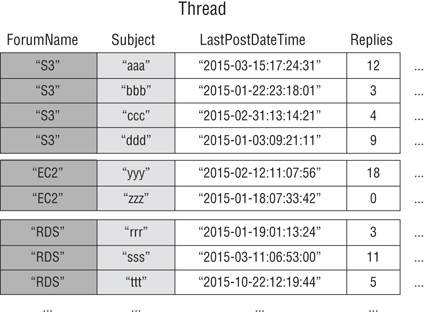
Figure 14.3 Forum thread table
DynamoDB stores all items with the same partition key value contiguously. In this example, given a particular ForumName, a Query operation could immediately locate the threads for that forum. Within a group of items with the same partition key value, the items are sorted by sort key value. If the sort key (Subject) is also provided in the Query operation, DynamoDB can narrow the results that are returned, such as returning the threads in the S3 forum that have a Subject beginning with the letter a.
Requests may require more complex data-access patterns, such as the following:
- Which forum threads receive the most views and replies?
- Which thread in a particular forum contains the largest number of messages?
- How many threads were posted in a particular forum, within a particular time period?
To answer these questions, the Query action would not be sufficient. Instead, you must scan the entire table. For a table with millions of items, this would consume a large amount of provisioned read throughput and time. However, you can configure one or more local secondary indexes on non-key attributes, such as Replies or LastPostDateTime.
A local secondary index maintains an alternate sort key for a given partition key value. A local secondary index also contains a copy of some, or all, of the attributes from its base table. You configure which attributes project into the local secondary index when you create the table. The data in a local secondary index is organized by the same partition key as the base table but with a different sort key. This enables you to access data items efficiently across this different dimension. For greater Query or Scan flexibility, create up to five local secondary indexes per table.
If an application locates the threads that have been posted within the last three months but lacks a local secondary index, the application must scan the entire thread table and discard any posts that were not listed within the specified time frame. With a local secondary index, a Query operation could use LastPostDateTime as a sort key and find the data quickly.
Figure 14.4 shows a local secondary index named LastPostIndex. The partition key is the same as that of the Thread table (see Figure 14.3), but the sort key is LastPostDateTime.

Figure 14.4 Last post index
Every local secondary index must meet the following conditions:
- The partition key is the same as that of its base table.
- The sort key consists of exactly one scalar attribute.
- The sort key of the base table projects into the index, where it acts as a non-key attribute.
In Figure 14.4, the partition key is ForumName, and the sort key of the local secondary index is LastPostDateTime. In addition, the sort key value from the base table (Subject) projects into the index, but it is not a part of the index key. If an application needs a list that is based on ForumName and LastPostDateTime, it can issue a Query request against LastPostIndex. The query results sort by LastPostDateTime and can return in ascending or descending order. The query can also apply key conditions, such as returning only items that have a LastPostDateTime within a particular time span.
Every local secondary index automatically contains the partition and sort keys from its base table, so you can project non-key attributes into the index. When you query the index, DynamoDB can retrieve these projected attributes efficiently. When you query a local secondary index, the Query operation can also retrieve attributes that do not project into the index. DynamoDB automatically collects these attributes from the base table but at a greater latency and with higher provisioned throughput costs.
![]() For any local secondary index, you can store up to 10 GB of data per distinct partition key value.
For any local secondary index, you can store up to 10 GB of data per distinct partition key value.
Creating a Local Secondary Index
To create one or more local secondary indexes on a table, use the LocalSecondaryIndexes parameter of the CreateTable operation. You create local secondary indexes when you create the table. When you delete a table, any local secondary indexes on that table are also deleted. Configure one non-key attribute to act as the sort key of the local secondary index. The local secondary indexes attribute is scalar and includes string, number, binary, document types, and set types. You can project attributes of any data type into a local secondary index.
![]() For tables with local secondary indexes, there is a 10-GB size limit per partition key value. A table with local secondary indexes can store any number of items, as long as the total size for any one partition key value does not exceed 10 GB.
For tables with local secondary indexes, there is a 10-GB size limit per partition key value. A table with local secondary indexes can store any number of items, as long as the total size for any one partition key value does not exceed 10 GB.
Querying a Local Secondary Index
In a DynamoDB table, the combined partition key value and sort key value for each item must be unique. However, in a local secondary index, the sort key value does not need to be unique for a given partition key value. If there are multiple items in the local secondary index that have the same sort key value, a Query operation returns all items with the same partition key value. In the response, the items that the query locates do not return in any particular order.
You can query a local secondary index using eventually consistent or strongly consistent reads. To configure which type of consistency you want, use the ConsistentRead parameter of the Query operation. A strongly consistent read from a local secondary index returns the latest updated values. If the Query operation must collect additional attributes from the base table, those attributes will be consistent with respect to the index.
Scanning a Local Secondary Index
You can use the Scan function to retrieve all data from a local secondary index. Provide the base table name and the index name in the request. With a Scan function, DynamoDB reads the data in the index and returns it to the application. You can also scan for specific data to return and discard the other data using the FilterExpression parameter of the Scan API.
Item Writes and Local Secondary Indexes
DynamoDB automatically keeps all local secondary indexes synchronized with their respective base tables. Applications seldom write directly to an index. However, understand the implications of how DynamoDB maintains these indexes.
When you create a local secondary index, configure an attribute to serve as the sort key for the index and configure a data type for that attribute. Whenever you write an item to the base table, if the item defines an index key attribute, its type must match the index key schema’s data type.
There is no requirement for a one-to-one relationship between the items in a base table and the items in a local secondary index. This behavior can be advantageous for many applications, because a table with many local secondary indexes incurs higher costs for write activity than tables with fewer indexes.
Provisioned Throughput for Local Secondary Indexes
When you create a table in DynamoDB, you provision read and write capacity units for the table’s expected workload, which includes read and write activity on the table’s local secondary indexes.
Read Capacity Units
When you query a local secondary index, the number of read capacity units consumed depends on how you access the data. As with table queries, an index query can use eventually consistent reads or strongly consistent reads, depending on the value of ConsistentRead. One strongly consistent read consumes one read capacity unit, but an eventually consistent read consumes only half of that. By choosing eventually consistent reads, you can reduce your read capacity unit charges.
For index queries that request only index keys and projected attributes, DynamoDB calculates the provisioned read activity in the same way that it does for queries against tables. However, the calculation is based on the sizes of the index entries instead of the size of the item in the base table. The number of read capacity units is the sum of all projected attribute sizes across all items returned. The result is then rounded up to the next 4-KB boundary.
For index queries that read, attributes do not project into the local secondary index, and DynamoDB must collect those attributes from the base table in addition to reading the projected attributes from the index. These collections occur when you include any non-projected [per DynamoDB documentation] attributes in the Select or ProjectionExpression parameters of the Query operation. Fetching causes additional latency in query responses, and it incurs a higher provisioned throughput cost. In addition to the reads from the local secondary index, you are charged for read capacity units for every base table item fetched. This charge is for reading each entire item from the table, not only the requested attributes.
The maximum size of the results returned by a Query operation is 1 MB. This includes the sizes of all of the attribute names and values across all items returned. However, if a query against a local secondary index causes DynamoDB to fetch item attributes from the base table, the maximum size of the data in the results may be lower. In this case, the result size is the sum of the following factors:
- The size of the matching items in the index, rounded up to the next 4 KB
- The size of each matching item in the base table, with each item individually rounded up to the next 4 KB
Using this formula, the maximum size of the results returned by a Query operation is still 1 MB.
Example 2: Query Read Capacity Units for Local Secondary Index
A table has items the size of 300 bytes. There is a local secondary index on that table, but only 200 bytes of each item projects into the index. If you query this index, the query requires table fetches for each item, and the query returns four items. DynamoDB sums up the following:
- Size of the matching items in the index: 200 bytes × 4 items = 800 bytes; this rounds up to 4 KB.
- Size of each matching item in the base table: (300 bytes, rounds up to 4 KB) × 4 items = 16 KB.
The total size of the data in the result is therefore 20 KB.
Write Capacity Units
When you add, update, or delete items in a table, the local secondary indexes consume provisioned write capacity units for the table. The total provisioned throughput cost for a write is the sum of write capacity units consumed by the write to the table and those consumed by the update of the local secondary indexes.
The cost of writing an item to a local secondary index depends on the following factors:
- If you write a new item to the table that defines an indexed attribute or you update an existing item to define a previously undefined indexed attribute, one write operation is required to put the item into the index.
- If an update to the table changes the value of an indexed key attribute (from A to B), two writes are required, one to delete the previous item from the index and another write to put the new item into the index.
- If an item was present in the index but a write to the table caused the indexed attribute to be deleted, one write is required to delete the old item projection from the index.
- If an item is not present in the index before or after the item update, there is no additional write cost for the index.
All of these factors assume that the size of each item in the index is less than or equal to the 1-KB item size for calculating write capacity units. Larger index entries require additional write capacity units. You can minimize your write costs by considering which attributes your queries must return and project only those attributes into the index.
Storage for Local Secondary Indexes
When an application writes an item to a table, DynamoDB automatically copies the correct subset of attributes to any local secondary indexes in which those attributes should appear. Your account is charged for storing the item in the base table and also for storing attributes in any local secondary indexes on that table.
The amount of space used by an index item is the sum of the following elements:
- Size in bytes of the base table primary key (partition and sort key)
- Size in bytes of the index key attribute
- Size in bytes of the projected attributes (if any)
- 100 bytes of overhead per index item
To estimate the storage requirements for a local secondary index, estimate the average size of an item in the index and then multiply by the number of items in the base table.
If a table contains an item where a particular attribute is not defined but that attribute is defined as an index sort key, then DynamoDB does not write any data for that item to the index.
Amazon DynamoDB Streams
Amazon DynamoDB Streams captures data modification events in DynamoDB tables. The data about these events appear in the stream in near real time and in the order that the events occurred.
Each event represents a stream record. When you enable a stream on a table, DynamoDB captures information about every modification to data items in the table. The stream captures an image of the entire item, including all of its attributes. A stream record contains information about a data modification to a single item in a DynamoDB table including the primary key attributes of the items. You can configure the stream so that the stream records capture additional information, such as the “before” and “after” images of modified items. Finally, a stream record is written when an item is deleted from the table, and each stream record also contains the name of the table, the event timestamp, and other metadata.
![]() Stream records have a lifetime of 24 hours, after which they are deleted automatically from the stream.
Stream records have a lifetime of 24 hours, after which they are deleted automatically from the stream.
A DynamoDB stream is a time-ordered flow of information of item-level modifications (create, update, or delete) to items in a DynamoDB table.
DynamoDB Streams does the following:
- Each stream record appears exactly once in the stream.
- For each item that is modified in a DynamoDB table, the stream records appear in the same sequence as the actual modifications to the item.
Many applications benefit from the ability to capture changes to items stored in a DynamoDB table when such changes occur. The following are common scenarios:
- An application in one AWS Region modifies the data in a Amazon DynamoDB table. A second application in another AWS Region reads these data modifications and writes the data to another table, creating a replica that stays in sync with the original table.
- A popular mobile app modifies data in a DynamoDB table at the rate of thousands of updates per second. Another application captures and stores data about these updates, providing near-real-time usage metrics for the mobile app.
- A global multiplayer game has a multi-master topology, storing data in multiple AWS Regions. Each master stays in sync by consuming and replaying the changes that occur in the remote regions.
- An application automatically sends notifications to the mobile devices of all friends in a group as soon as one friend uploads a new picture.
- A new customer adds data to a DynamoDB table. This event invokes another application that sends a welcome email to the new customer.
Whenever an application creates, updates, or deletes items in the table, Amazon DynamoDB Stream writes a stream record with the primary key attribute, or attributes, of the items that were modified. A stream record contains information about a data modification to a single item in a DynamoDB table. Applications can access this log and view the data items as they appeared before and after they were modified, in near real time.
![]() DynamoDB Streams writes stream records in near-real time, so you can build applications that consume these streams and act based on the contents.
DynamoDB Streams writes stream records in near-real time, so you can build applications that consume these streams and act based on the contents.
DynamoDB Cross-Region Replication
You can create tables that automatically replicate across two or more AWS Regions with full support for multi-master writes. Using cross-region replication, you can build fast, massively scaled applications for a global user base without having to manage the replication process.
DynamoDB Stream Endpoints
AWS maintains separate endpoints for DynamoDB and DynamoDB Streams. To work with database tables and indexes, your application must access a DynamoDB endpoint. To read and process DynamoDB Streams records, your application must access a DynamoDB Streams endpoint in the same AWS Region.
Figure 14.5 shows the DynamoDB endpoint flow.

Figure 14.5 DynamoDB Streams endpoints
The naming convention for DynamoDB Streams endpoints is streams.dynamodb.<region>.amazonaws.com. For example, if you use the endpoint dynamodb.us-west-2.amazonaws.com to access DynamoDB, use the endpoint streams .dynamodb.us-west-2.amazonaws.com to access DynamoDB Streams.
The AWS SDKs provide separate clients for DynamoDB and DynamoDB Streams. Depending on your requirements, your application can access a DynamoDB endpoint, a DynamoDB Streams endpoint, or both at the same time. To connect to both endpoints, your application must instantiate two clients: one for DynamoDB and one for DynamoDB Streams.
Enabling a Stream
You can enable a stream on a new table when you create it, enable or disable a stream on an existing table, or change the settings of a stream. DynamoDB Streams operates asynchronously, so there is no performance impact on a table if you enable a stream.
You can also use the CreateTable or UpdateTable APIs to enable or modify a stream. The StreamSpecification parameter determines how the stream is configured:
- StreamEnabled Specifies whether a stream for the table is enabled (true) or disabled (false)
- StreamViewType Specifies the information that will be written to the stream whenever data in the table is modified:
- KEYS_ONLY Only the key attributes of the modified item
- NEW_IMAGE The entire item as it appears after it was modified
- OLD_IMAGE The entire item as it appeared before it was modified
- NEW_AND_OLD_IMAGES Both the new and the old images of the item
You can enable or disable a stream at any time. However, if you attempt to enable a stream on a table that already has a stream, you will receive a ResourceInUseException. If you attempt to disable a stream on a table that does not have a stream, you will receive a ValidationException.
When you set StreamEnabled to true, DynamoDB creates a new stream with a unique stream descriptor. If you disable and then re-enable a stream on the table, a new stream is created with a different stream descriptor.
The Amazon Resource Name (ARN) uniquely identifies every stream. The following is an example of defining an ARN for a stream on a DynamoDB table named TestTable:
arn:aws:dynamodb:us-west-2:111122223333:table/TestTable/stream/ 2015-05-11T21:21:33.291
To determine the latest stream descriptor for a table, issue a DynamoDB DescribeTable request and look for the LatestStreamArn element in the response.
Reading and Processing a Stream
To read and process a stream, your application must connect to a DynamoDB Streams endpoint and issue API requests. A stream consists of stream records. Each stream record represents a single data modification in the DynamoDB table to which the stream belongs. Each stream record is assigned a sequence number, reflecting the order in which the record was published to the stream.
Stream records are organized into groups called shards. Each shard acts as a container for multiple stream records and contains information required for accessing and iterating through these records. The stream records within a shard are removed automatically after 24 hours. If you disable a stream, any shards that are open are closed.
Shards are ephemeral, meaning that they can be both created and deleted automatically as necessary. Any shard can automatically split into multiple new shards, and a shard may split in response to high levels of write activity on its parent table to enable applications to process records from multiple shards in parallel.
It is equally possible for a parent shard to have only one child shard. Because shards have a parent-and-children lineage, an application must always process a parent shard before it processes a child shard. This ensures that the stream records process in the correct order.
If you use the DynamoDB Streams Kinesis Adapter, this processing is handled for you. Your application processes the shards and stream records in the correct order, and it automatically handles new or expired shards and shards that split while the application is running.
Figure 14.6 shows the relationship between a stream, shards in the stream, and stream records in the shards.

Figure 14.6 Stream and shard relationship
To access a stream and process the stream records, do the following:
- Identify the unique ARN of the stream that you want to access.
- Determine which shard or shards in the stream contain the stream records of interest.
- Access the shard or shards and retrieve the stream records that you want.
![]() If you perform a PutItem or UpdateItem operation that does not change any data in an item, then DynamoDB Streams will not write a stream record for that operation.
If you perform a PutItem or UpdateItem operation that does not change any data in an item, then DynamoDB Streams will not write a stream record for that operation.
![]() No more than two processes should be reading from the same stream’s shard at the same time. Having more than two readers per shard may result in throttling.
No more than two processes should be reading from the same stream’s shard at the same time. Having more than two readers per shard may result in throttling.
Read Capacity for DynamoDB Streams
DynamoDB is available in multiple AWS Regions around the world. Each region is independent and isolated from other AWS Regions. For example, a table called People in the us-east-2 Region and a table named People in the us-west-2 Region are two entirely separate tables.
Every AWS Region consists of multiple, distinct locations called Availability Zones. Each Availability Zone is isolated from failures in other Availability Zones and provides inexpensive, low-latency network connectivity to other Availability Zones in the same region. This allows rapid replication of your data among multiple Availability Zones in a region.
When an application writes data to a DynamoDB table and receives an HTTP 200 response (OK), all copies of the data are updated. The data is eventually consistent across all storage locations, usually within one second or less.
Eventually consistent reads DynamoDB supports eventually consistent reads and strongly consistent reads. When you read data from a DynamoDB table, the response may not reflect the results of a recently completed write operation and may include some stale data. If you repeat your read request after a short period, the response returns the latest data.
Strongly consistent reads DynamoDB uses eventually consistent reads unless you specify otherwise. Read operations, such as GetItem, query, and Scan, provide a ConsistentRead parameter. If you set this parameter to true, DynamoDB uses strongly consistent reads during the operation. When you request a strongly consistent read, DynamoDB returns a response with the most up-to-date data, reflecting the updates from all prior write operations that were successful. A strongly consistent read may not be available if there is a network delay or outage.
DynamoDB Streams API
The DynamoDB Streams API provides the following operations:
ListStreams Returns a list of stream descriptors for the current account and endpoint, or you can request only the stream descriptors for a particular table name.
DescribeStream Returns information about a stream, such as its ARN, and where your application can begin to read the first few stream records. The output includes a list of shards associated with the stream, including the shard IDs.
GetShardIterator Returns a shard iterator, which describes a location within a shard, to retrieve the records from the stream. You can request that the iterator provide access to the oldest point, the newest point, or a particular point in the stream.
GetRecords Retrieves one or more stream records by using a given shard iterator. Provides the shard iterator returned from a GetShardIterator request.
Data Retention Limit for DynamoDB Streams
All data in DynamoDB Streams is subject to a 24-hour lifetime. You can retrieve and analyze the last 24 hours of activity for any given table; however, data older than 24 hours is susceptible to trimming (removal) at any moment.
If you disable a stream on a table, the data in the stream continues to be readable for 24 hours. After this time, the data expires, and the stream records are deleted automatically. There is no mechanism for manually deleting an existing stream; you must wait until the retention limit expires (24 hours) and all of the stream records are deleted.
AWS Lambda Triggers in DynamoDB Streams
DynamoDB integrates with AWS Lambda, so you can create triggers (code that executes automatically) that automatically respond to events in DynamoDB Streams. With triggers, you can build applications that react to data modifications in DynamoDB tables.
Example 3: DynamoDB Table Update Using AWS Lambda and Amazon Resource Name
In Figure 14.2, you have a mobile gaming app that writes to a GameScores table. Whenever the TopScore attribute of the GameScores table updates, a corresponding stream record writes to the table’s stream. This event triggers a Lambda function that posts a congratulatory message on a social media network.
If you enable DynamoDB Streams on a table, you can associate the stream Amazon ARN with a Lambda function that you write. Immediately after an item in the table is modified, a new record appears in the table’s stream. Lambda polls the stream and invokes your Lambda function synchronously when it detects new stream records.
The Lambda function can perform any actions that you configure, such as sending a notification or initiating a workflow. For instance, you can write a Lambda function to copy each stream record to persistent storage, such as Amazon Simple Storage Service (Amazon S3), to create a permanent audit trail of write activity in your table.
Query so you can create triggers that automatically respond to events in DynamoDB Streams. With triggers, you can build applications that react to data modifications in DynamoDB tables.
If you enable DynamoDB Streams on a table, you can associate the stream ARN with a Lambda function that you write. Immediately after an item in the table is modified, a new record appears in the table’s stream. Lambda polls the stream and invokes your Lambda function synchronously when it detects new stream records.
Example 4: Lambda Email Trigger
A Customers table, such as the one shown in Figure 14.7, contains customer information for a company. If you want to send a “welcome” email to each new customer, enable a stream on that table and then associate the stream with a Lambda function. The Lambda function executes whenever a new stream record appears, but it processes only new items added to the Customers table. For any item that has an EmailAddress attribute, the Lambda function invokes Amazon Simple Email Service (Amazon SES) to send an email to that address. In Figure 14.7, the last customer, Craig Roe, will not receive an email because he does not have an EmailAddress.

Figure 14.7 AWS Lambda Customers table
Amazon DynamoDB Auto Scaling
Amazon DynamoDB automatic scaling actively manages throughput capacity for tables and global secondary indexes. With automatic scaling, you can define a range (upper and lower limits) for read and write capacity units and define a target utilization percentage within that range. DynamoDB automatic scaling seeks to maintain your target utilization, even as your application workload increases or decreases.
With DynamoDB automatic scaling, a table or a global secondary index can increase its provisioned read and write capacity to handle sudden increases in traffic without throttling. When the workload decreases, DynamoDB automatic scaling can decrease the throughput so that you do not pay for unused provisioned capacity.
If you use the AWS Management Console to create a table or a global secondary index, DynamoDB automatic scaling is enabled by default. You can manage automatic scaling settings at any time by using the console, the AWS CLI, or one of the AWS SDKs.
Managing Throughput Capacity Automatically with AWS Auto Scaling
Many database workloads are cyclical in nature or are difficult to predict in advance. In a social networking application, where most of the users are active during daytime hours, the database must be able to handle the daytime activity. But there is no need for the same levels of throughput at night. If a new mobile gaming app is experiencing rapid adoption and becomes too popular, the app could exceed the available database resources, resulting in slow performance and unhappy customers. These situations often require manual intervention to scale database resources up or down in response to varying usage levels.
DynamoDB uses the AWS Application Auto Scaling service to adjust provisioned throughput capacity dynamically in response to actual traffic patterns. This enables a table or a global secondary index to increase its provisioned read and write capacity to handle sudden increases in traffic, without throttling. When the workload decreases, Application Auto Scaling decreases the throughput so that you do not pay for unused provisioned capacity.
Application Auto Scaling does not scale down your provisioned capacity if the consumed capacity of your table becomes zero. To scale down capacity manually, perform one of the following actions:
- Send requests to the table until automatic scaling scales down to the minimum capacity.
- Change the policy and reduce the maximum provisioned capacity to the same size as the minimum provisioned capacity.
With Application Auto Scaling, you can create a scaling policy for a table or a global secondary index. The scaling policy specifies whether you want to scale read capacity or write capacity (or both), and the minimum and maximum provisioned capacity unit settings for the table or index.
The scaling policy also contains a target utilization that is the percentage of consumed provisioned throughput at a point in time. Application Auto Scaling uses a target tracking algorithm to adjust the provisioned throughput of the table (or index) upward or downward in response to actual workloads so that the actual capacity utilization remains at or near your target utilization.
DynamoDB automatic scaling also supports global secondary indexes. Every global secondary index has its own provisioned throughput capacity, separate from that of its base table. When you create a scaling policy for a global secondary index, Application Auto Scaling adjusts the provisioned throughput settings for the index to ensure that its actual utilization stays at or near your desired utilization ratio, as shown in Figure 14.8.

Figure 14.8 DynamoDB Auto Scaling
How DynamoDB Auto Scaling Works
The steps in Figure 14.8 summarize the automatic scaling process:
- Create an Application Auto Scaling policy for your DynamoDB table.
- DynamoDB publishes consumed capacity metrics to Amazon CloudWatch.
- If the table’s consumed capacity exceeds your target utilization (or falls below the target) for a specific length of time, CloudWatch triggers an alarm. You can view the alarm on the AWS Management Console and receive notifications using Amazon Simple Notification Service (Amazon SNS).
- The CloudWatch alarm invokes Application Auto Scaling to evaluate your scaling policy.
- Application Auto Scaling issues an UpdateTable request to adjust your table’s provisioned throughput.
- DynamoDB processes the UpdateTable request, increasing or decreasing the table’s provisioned throughput capacity dynamically so that it approaches your target utilization.
DynamoDB automatic scaling modifies provisioned throughput settings only when the actual workload stays elevated or depressed for a sustained period of several minutes. The Application Auto Scaling target tracking algorithm seeks to keep the target utilization at or near your chosen value over the long term. Sudden, short-duration spikes of activity are accommodated by the table’s built-in burst capacity.
Burst Capacity
DynamoDB provides some flexibility in your per-partition throughput provisioning by providing burst capacity. Whenever you are not fully using a partition’s throughput, Amazon DynamoDB reserves a portion of that unused capacity for later bursts of throughput to handle usage spikes.
DynamoDB currently retains up to 5 minutes (300 seconds) of unused read and write capacity. During an occasional burst of read or write activity, these extra capacity units can be consumed quickly—even faster than the per-second provisioned throughput capacity that you have defined for your table. However, do not rely on burst capacity being available at all times, as DynamoDB can also consume burst capacity for background maintenance and other tasks without prior notice.
To enable DynamoDB automatic scaling, you create a scaling policy. This scaling policy specifies the table or global secondary index that you want to manage, which capacity type to manage (read or write capacity), the upper and lower boundaries for the provisioned throughput settings, and your target utilization.
When you create a scaling policy, Application Auto Scaling creates a pair of CloudWatch alarms on your behalf. Each pair represents your upper and lower boundaries for provisioned throughput settings. These CloudWatch alarms are triggered when the table’s actual utilization deviates from your target utilization for a sustained period of time.
When one of the CloudWatch alarms is triggered, Amazon SNS sends you a notification (if you have enabled it). The CloudWatch alarm then invokes Application Auto Scaling, which notifies DynamoDB to adjust the table’s provisioned capacity upward or downward, as appropriate.
Considerations for DynamoDB Auto Scaling
Before you begin using DynamoDB automatic scaling, be aware of the following:
- DynamoDB automatic scaling can increase read capacity or write capacity as often as necessary in accordance with your automatic scaling policy. All DynamoDB limits remain in effect.
- DynamoDB automatic scaling does not prevent you from manually modifying provisioned throughput settings. These manual adjustments do not affect any existing CloudWatch alarms that are related to DynamoDB automatic scaling.
- If you enable DynamoDB automatic scaling for a table that has one or more global secondary indexes, AWS highly recommends that you also apply automatic scaling uniformly to those indexes. You can apply this by choosing Apply same settings to global secondary indexes in the AWS Management Console.
Provisioned Throughput for DynamoDB Auto Scaling
If you are not using DynamoDB automatic scaling, you must manually define your throughput requirements. Provisioned throughput is the maximum amount of capacity that an application can consume from a table or index. If your application exceeds your provisioned throughput settings, it is subject to request throttling.
Example 5: Determining the Provisioned Throughput Setting
Suppose that you want to read 80 items per second from a table, where the items are 3 KB in size, and you want strongly consistent reads with each read requiring one provisioned read capacity unit. To determine this, divide the item size of the operation by 4 KB and then round up to the nearest whole number:
3 KB/4 KB = 0.75, or 1 read capacity unit
Knowing this, you must set the table’s provisioned read throughput to 80 read capacity units:
1 read capacity unit per item × 80 reads per second = 80 read capacity units
If you want to write 100 items per second to your table, and the items are 512 bytes in size, each write requires one provisioned write capacity unit. To determine this, divide the item size of the operation by 1 KB and then round up to the nearest whole number:
512 bytes/1 KB = 0.5, or 1
To accomplish this, set the table’s provisioned write throughput to 100 write capacity units:
1 write capacity unit per item × 100 writes per second = 100 write capacity units
Partitions and Data Distribution
DynamoDB stores data in partitions. A partition is an allocation of storage for a table, backed by solid-state drives (SSDs) and automatically replicated across multiple Availability Zones within an AWS Region. Partition management is handled entirely by DynamoDB, so you do not have to manage partitions yourself. When you create a table, the initial status of the table is CREATING. During this phase, DynamoDB allocates sufficient partitions to the table so that it can handle your provisioned throughput requirements. You can begin writing and reading table data after the table status changes to ACTIVE.
DynamoDB allocates additional partitions to a table in the following situations:
- If you increase the table’s provisioned throughput settings beyond what the existing partitions can support
- If an existing partition fills to capacity and more storage space is required
Partition management occurs automatically in the background, and it is transparent to your applications. Your table remains available throughout and fully supports your provisioned throughput requirements. Global secondary indexes in DynamoDB are also composed of partitions. The data in a global secondary index is stored separately from the data in its base table, but index partitions behave similarly to table partitions.
Data Distribution: Partition Key
If your table has a simple primary key (partition key only), DynamoDB stores and retrieves each item based on its partition key value. To write an item to the table, DynamoDB uses the value of the partition key as input to an internal hash function. The output value from the hash function determines the partition in which the item will be stored. To read an item from the table, you must configure the partition key value for the item. DynamoDB uses this value as input to its hash function, yielding the partition in which the item can be found.
Figure 14.9 shows a table named Pets, which spans multiple partitions. The table’s primary key is AnimalType (only this key attribute is shown). DynamoDB uses its hash function to determine where to store a new item, in this case based on the hash value of the string Dog. The items are not stored in sorted order. Each item’s location is determined by the hash value of its partition key.

Figure 14.9 Data distribution and partition
![]() DynamoDB is optimized for uniform distribution of items across a table’s partitions, regardless of the number of partitions. Choose a partition key with a large number of distinct values relative to the number of items in the table.
DynamoDB is optimized for uniform distribution of items across a table’s partitions, regardless of the number of partitions. Choose a partition key with a large number of distinct values relative to the number of items in the table.
Data Distribution: Partition Key and Sort Key
If the table has a composite primary key (partition key and sort key), DynamoDB calculates the hash value of the partition key in the same way, but it stores the items with the same partition key value physically close together, ordered by sort key value.
To write an item to the table, DynamoDB calculates the hash value of the partition key to determine which partition should contain the item. In that partition, there could be several items with the same partition key value, so DynamoDB stores the item among the others with the same partition key in ascending order by sort key.
To read an item from the table, configure both the partition key value and sort key value. DynamoDB calculates the partition key’s hash value, yielding the partition in which the item can be found.
You can read multiple items from the table in a single Query operation, if the desired items have the same partition key value. DynamoDB returns all items with that partition key value. You can apply a condition to the sort key that only returns items within a certain range of values.
Optimistic Locking with Version Number
Optimistic locking is a strategy to ensure that the client-side item that you are updating or deleting is the same as the item in DynamoDB. If you use this strategy, then all writes on your database are protected from being accidentally overwritten.
![]() DynamoDB global tables use a “last writer wins” reconciliation between concurrent updates. If you use Global Tables, last writer policy wins. In this case, the locking strategy does not work as expected.
DynamoDB global tables use a “last writer wins” reconciliation between concurrent updates. If you use Global Tables, last writer policy wins. In this case, the locking strategy does not work as expected.
With optimistic locking, each item has an attribute that acts as a version number. If you retrieve an item from a table, the application records the version number of that item. You can update the item, but only if the version number on the server side has not changed. If there is a version mismatch, then someone else has modified the item before you did, and the update attempt fails because you have an outdated version of the item. If this happens, you retrieve the current item and then attempt to update it again.
To support optimistic locking, the AWS SDK for Java provides the @Amazon DynamoDBVersionAttribute annotation. In the mapping class for your table, designate one property to store the version number and mark it using the annotation. When you save an object, the corresponding item in the DynamoDB table has an attribute that stores the version number. The Amazon DynamoDBMapper assigns a version number when you first save the object, and it automatically increments the version number each time you update the item. Your update or delete requests succeed only if the client-side object version matches the corresponding version number of the item in the Amazon DynamoDB table.
ConditionalCheckFailedException occurs if the following conditions are true:
- You use optimistic locking with @Amazon DynamoDBVersionAttribute, and the version value on the server is different from the value on the client side.
- You configure your own conditional constraints while saving data by using Amazon DynamoDBMapper with Amazon DynamoDBSaveExpression, and these constraints failed.
Disabling Optimistic Locking
To disable optimistic locking, change the Amazon DynamoDBMapperConfig.SaveBehavior enumeration value from UPDATE to CLOBBER. Do this by creating an Amazon DynamoDBMapperConfig instance that skips version checking and then use this instance for your requests. You can also set locking behavior for a specific operation only. For example, the following Java snippet uses the DynamoDBMapper to save a catalog item. It specifies DynamoDBMapperConfig.SaveBehavior by adding the optional DynamoDBMapperConfig parameter to the save method.
DynamoDBMapper mapper = new DynamoDBMapper(client);// Load a catalog item.CatalogItem item = mapper.load(CatalogItem.class, 101);item.setTitle("This is a new title for the item");...// Save the item.mapper.save(item,new DynamoDBMapperConfig(DynamoDBMapperConfig.SaveBehavior.CLOBBER));
DynamoDB Tags
You can label DynamoDB resources with tags. Tags allow you to categorize your resources in different ways: by purpose, owner, environment, or other criteria. Tags help you to identify a resource quickly based on the tags that you have assigned to it, and they help you to see your AWS bills broken down by tags.
Tables that have tags automatically tag local secondary indexes and global secondary indexes. Currently, you cannot tag DynamoDB Streams. AWS offerings and services, such as Amazon EC2, Amazon S3, DynamoDB, and more, support tags. Efficient tagging can provide cost insights by enabling you to create reports across services that carry a specific tag.
Tag Restrictions
Each tag consists of a key and a value, both of which you define. Each DynamoDB table can have only one tag with the same key, so if you attempt to add an existing tag (the same key), the existing tag value updates to the new value.
The following restrictions apply:
- Tag keys and values are case-sensitive.
- The maximum key length is 128 Unicode characters, and the maximum value length is 256 Unicode characters. The allowed character types are letters, white space, and numbers, plus the following special characters: + - = . _ : /.
- The maximum number of tags per resource is 50.
- The AWS-assigned tag names and values are automatically assigned the aws: prefix, which you cannot manually assign.
- AWS-assigned tag names do not count toward the tag limit of 50.
- User-assigned tag names have the prefix user: in the cost allocation report.
- You cannot tag a resource at the same time that you create it.
![]() Tagging is a separate action that you can perform only after you create the resource. You cannot backdate the application of a tag.
Tagging is a separate action that you can perform only after you create the resource. You cannot backdate the application of a tag.
DynamoDB Items
A DynamoDB item is a collection of attributes that is uniquely identifiable among all other entities in the table, and each item has a name and a value. An attribute value can be a scalar, a set, or a document type. Each table contains zero or more items. For example, in a People table, each item represents a person, and in a “cars” table, each item represents one vehicle. Items in DynamoDB are similar to rows, records, or tables in other database systems, but in DynamoDB, there is no limit to the number of items that you can store in a table.
Atomic Counters
You can use the UpdateItem operation to implement an atomic counter, which is a numeric attribute that increments, unconditionally, without interfering with other write requests. With an atomic counter, the updates are not independent, and the numeric value increments each time that you call UpdateItem.
You can use an atomic counter to track the number of visitors to a website. In this case, your application would increment a numeric value, regardless of its current value. If an UpdateItem operation fails, the application may retry the operation. This would risk updating the counter twice, but most can tolerate a slight overcounting or undercounting of website visitors.
An atomic counter would not be appropriate where overcounting or undercounting cannot be tolerated, as in a banking application. In this case, it is safer to use a conditional update instead of an atomic counter.
![]() All write requests are applied in the order in which they were received.
All write requests are applied in the order in which they were received.
Conditional Writes
By default, the DynamoDB write operations (PutItem, UpdateItem, DeleteItem) are unconditional. Each of these operations overwrites an existing item that has the specified primary key. DynamoDB supports conditional writes for these operations. A conditional write succeeds only if the item attributes meet one or more expected conditions; otherwise, it returns an error.
Conditional writes are helpful in many situations, including cases in which multiple users attempt to modify the same item. You may want a PutItem operation to succeed only if there is not already an item with the same primary key. Alternatively, you could prevent an UpdateItem operation from modifying an item if one of its attributes has a certain value. Consider Figure 14.10 in which two users (Alice and Bob) are working with the same item from a DynamoDB table.

Figure 14.10 Conditional write success
Suppose that Alice updates the Price attribute to 8.
aws dynamodb update-item--table-name ProductCatalog--key '{"Id":{"N":"1"}}'--update-expression "SET Price = :newval"--expression-attribute-values file://expression-attribute-values.json
The arguments for --expression-attribute-values write to the file expression-attribute-values.json.
{":newval":{"N":"8"}}
Now suppose that Bob issues a similar UpdateItem request later but changes the Price to 12. For Bob, the --expression-attribute-values parameter looks like this:
{":newval":{"N":"12"}}
Bob’s request succeeds, but Alice’s earlier update is lost.
To request a conditional PutItem, DeleteItem, or UpdateItem, you configure a condition expression. A condition expression is a string containing attribute names, conditional operators, and built-in functions where the entire expression must evaluate to true; otherwise, the operation fails.
Now consider Figure 14.11, showing how conditional writes would prevent Alice’s update from being overwritten.

Figure 14.11 Conditional write success
Alice first attempts to update Price to 8 but only if the current Price is 10.
aws dynamodb update-item--table-name ProductCatalog--key '{"Id":{"N":"1"}}'--update-expression "SET Price = :newval"--condition-expression "Price = :currval"--expression-attribute-values file://expression-attribute-values.json
The arguments for --expression-attribute-values write to the file expression-attribute-values.json.
{":newval":{"N":"8"},":currval":{"N":"10"}}
Alice’s update succeeds because the condition evaluates to true.
Next, Bob attempts to update the Price to 12 but only if the current Price is 10. For Bob, the --expression-attribute-values parameter looks like the following:
{":newval":{"N":"12"},":currval":{"N":"10"}}
Because Alice has previously changed the Price to 8, the condition expression evaluates to false and Bob’s update fails.
Time to Live
Time to Live (TTL) for DynamoDB enables you to define when items in a table expire so that they can be automatically deleted from the database.
AWS provides TTL at no extra cost to you as a way to reduce both storage usage and the cost of storing irrelevant data without using provisioned throughput. With TTL enabled on a table, you can set a timestamp for deletion on a per-item basis and limit storage usage to only those records that are relevant.
TTL is useful if you have continuously accumulating data that loses relevance after a specific time, such as session data, event logs, usage patterns, and other temporary data. If you have sensitive data that must be retained only for a certain amount of time according to contractual or regulatory obligations, TTL helps you to make sure that data is removed promptly and on schedule.
Enabling Time to Live
When you enable TTL on a table, a background job checks the TTL attribute of items to determine whether they are expired. TTL compares the current time in epoch time format to the time stored in the Time to Live attribute of an item. If the epoch time value stored in the attribute is less than the current time, the item is marked as expired and later deleted.
![]() The epoch time format is the number of seconds elapsed since 12:00:00 a.m. on January 1, 1970, UTC.
The epoch time format is the number of seconds elapsed since 12:00:00 a.m. on January 1, 1970, UTC.
DynamoDB deletes expired items on a best-effort basis to ensure availability of throughput for other data operations. DynamoDB typically deletes expired items within 48 hours of expiration. The exact duration within which an item is deleted after expiration is specific to the nature of the workload and the size of the table.
Items that have expired but not deleted still show up in reads, queries, and scans. These items can be updated, and successful updates to change or remove the expiration attribute will be honored. As items are deleted, they are immediately removed from local secondary and global secondary indexes in the same eventually consistent way as a standard delete operation.
Before Using Time to Live
Before you enable TTL on a table, consider the following:
- Make sure that any existing timestamp values in the specified Time to Live attribute are correct and in the right format.
- Items with an expiration time greater than five years in the past are not deleted.
- If data recovery is a concern, back up your table.
- For a 24-hour recovery window, use DynamoDB Streams.
- For a full backup, use AWS Data Pipeline.
- Use the AWS CloudFormation to set TTL when you create a DynamoDB table.
- Use Identity and Access Management (IAM) policies to prevent unauthorized updates to the TTL attribute or configuration of the TTL feature. If you allow access to only specified actions in your existing IAM policies, ensure that your policies update to allow DynamoDB:UpdateTimeToLive for roles that need to enable or disable TTL on tables.
- Consider whether you must complete any post-processing of deleted items. The stream’s records of TTL deletes are marked, and you use AWS Lambda function to monitor the records.
When your program sends a request, DynamoDB attempts to process it. If the request is successful, DynamoDB returns an HTTP success status code (200 OK), along with the results from the requested operation.
If the request is unsuccessful, DynamoDB returns an error. Each error has three components:
- An HTTP status code (such as 400)
- An exception name (such as ResourceNameNotFound)
- An error message (such as Requested resource not found: Table: tablename not found)
The AWS SDKs resolve propagating errors in your application so that you can take appropriate action. For example, in a Java program, write try-catch logic to handle a ResourceNotFoundException.
Error Handling in Your Application
For your application to run smoothly, you must add logic to catch and respond to errors. Typical approaches include using try-catch blocks or if-then statements. The AWS SDKs perform their own retries and error checking. If you encounter an error while using one of the AWS SDKs, the error code and description help you troubleshoot it. You may also see a Request ID in the response, which can be helpful when working with AWS Support to diagnose an issue.
Error Retries and Exponential Backoff
Numerous components on a network, such as DNS servers, switches, load balancers, and others, can return error responses anywhere in the life of a given request. The usual technique for dealing with these error responses in a networked environment is to implement retries in the client application. This technique increases the reliability of the application and reduces operational costs for the developer.
As each AWS SDK automatically implements retry logic, you can modify the retry parameters to suit your needs. For example, consider a Java application that requires a fail-fast strategy with no retries allowed in case of an error. With the AWS SDK for Java, you could use the ClientConfiguration class and provide a maxErrorRetry value of 0 to turn off the retries.
If you are not using an AWS SDK, attempt to retry original requests that receive server errors (5xx). However, client errors (4xx), other than a ThrottlingException or a ProvisionedThroughputExceededException, indicate the need to revise the request itself or to correct the problem before trying again.
In addition to simple retries, each AWS SDK implements the exponential backoff algorithm for better flow control. The concept behind exponential backoff is to use progressively longer waits between retries for consecutive error responses. For example, you can set the wait to up to 50 milliseconds before the first retry, up to 100 milliseconds before the second retry, up to 200 milliseconds before third retry, and so on.
However, if the request has not succeeded after a minute, the request size may exceed your provisioned throughput and not the request rate. Set the maximum number of retries to stop at around one minute. If the request is not successful, investigate your provisioned throughput options.
Capacity Units Consumed by Conditional Writes
If a ConditionExpression generates an evaluation of false during a conditional write, DynamoDB consumes write capacity from the table. If the item does not currently exist in the table, DynamoDB consumes one write capacity unit. If the item does exist, then the number of write capacity units consumed depends on the size of the item. A failed conditional write of a 1-KB item would consume one write capacity unit. If the item were twice that size, the failed conditional write would consume two write capacity units.
A failed conditional write returns a ConditionalCheckFailedException. When this occurs, you will not receive information in the response about the write capacity that was consumed. However, you can view the ConsumedWriteCapacityUnits metric for the table in Amazon CloudWatch.
To return the number of write capacity units consumed during a conditional write, you use the ReturnConsumedCapacity parameter with the following attributes:
- Total Returns the total number of write capacity units consumed.
- Indexes Returns the total number of write capacity units consumed with subtotals for the table and any secondary indexes that were affected by the operation.
- None No write capacity details are returned (default).
![]() Write operations consume only write capacity units; they do not consume read capacity units.
Write operations consume only write capacity units; they do not consume read capacity units.
Unlike a global secondary index, a local secondary index shares its provisioned throughput capacity with its table. Read and write activity on a local secondary index consumes provisioned throughput capacity from the table.
Configuring Item Attributes
This section describes how to refer to item attributes in an expression and projection expression. You can work with any attribute, even if it is deeply nested within multiple lists and maps.
Item Attributes
You can work with any attribute in an expression, even if it is deeply nested within multiple lists and maps.
Top-Level Attributes
If an attribute is not embedded within another attribute, the attribute is top level. Top-level attributes include the following:
- Id
- Title
- Description
- BicycleType
- Brand
- Price
- Color
- ProductCategory
- InStock
- QuantityOnHand
- RelatedItems
- Pictures
- ProductReviews
- Comment
- Safety.Warning
All of the top-level attributes are scalars, except for Color (list), RelatedItems (list), Pictures (map), and ProductReviews (map).
Nested Attributes
A nested attribute is embedded within another attribute. To access a nested attribute, you use dereference operators:
- [n] for list elements
- .(dot) for map elements
Accessing List Elements
The dereference operator for a list element is [n], where n is the element number. List elements are zero-based, so [0] represents the first element in the list, [1] represents the second, and so on. For example:
- MyList[0]
- AnotherList[12]
- ThisList[5][11]
The element ThisList[5] is itself a nested list. Therefore, ThisList[5][11] refers to the twelfth element in that list.
The number within the square brackets must be a non-negative integer. Therefore, the following expressions are invalid:
- MyList[-1]
- MyList[0.4]
Accessing Map Elements
The dereference operator for a map element is a dot (.). Use a dot as a separator between elements in a map. For example:
- MyMap.nestedField
- MyMap.nestedField.deeplyNestedField
Document Paths
In an expression, you use a document path to tell DynamoDB where to find an attribute. For a top-level attribute, the document path is the attribute name. For a nested attribute, you construct the document path by using dereference operators.
The following are examples of document paths:
- Top-level scalar attribute: ProductDescription.
- Top-level list attribute returns the entire list, not only some of the elements: RelatedItems.
- Third element from the RelatedItems list (remember that list elements are zero-based): RelatedItems[2].
- Front-view picture of the product: Pictures.FrontView.
- All of the five-star reviews: ProductReviews.FiveStar.
- First of the five-star reviews: ProductReviews.FiveStar[0].
You can use any attribute name in a document path if the first character is a–z or A–Z and the second character (if present) is a–z, A–Z, or 0–9. If an attribute name does not meet this requirement, define an expression attribute name as a placeholder.
![]() The maximum depth for a document path is 32. Therefore, the number of dereference operators in a path cannot exceed this limit.
The maximum depth for a document path is 32. Therefore, the number of dereference operators in a path cannot exceed this limit.
Expressions
In DynamoDB, you can use expressions to denote the attributes that you want to read from an item. To indicate any conditions that must be met (conditional update) and to indicate how the attributes are to be updated, you can also use expressions when writing an item.
![]() For backward-compatibility, DynamoDB also supports conditional parameters that do not use expressions. New applications should use expressions instead of the legacy parameters.
For backward-compatibility, DynamoDB also supports conditional parameters that do not use expressions. New applications should use expressions instead of the legacy parameters.
Item Projection Expressions
To read data from a table, use operations such as GetItem, Query, or Scan. DynamoDB returns all of the item attributes by default. To acquire select attributes, use a projection expression.
A projection expression is a string that identifies the attributes that you want to collect. To retrieve a single attribute, specify its name. For multiple attributes, the names must be comma-separated.
The following are examples of projection expressions:
- Single top-level attribute:
- Title
- Three top-level attributes; DynamoDB retrieves the entire Color set:
- Title, Price, Color
- Four top-level attributes’ DynamoDB returns the entire contents of RelatedItems and ProductReviews:
- Title, Description, RelatedItems, ProductReviews
Attribute Names in a Projection Expression
You can use any attribute name in a projection expression, where the first character is a–z or A–Z and the second character (if present) is a–z, A–Z, or 0–9. If an attribute name does not meet this requirement, you must define an expression attribute name as a placeholder.
Expression Attribute Names
An expression attribute name is a placeholder that you use in an expression as an alternative to an actual attribute name. An expression attribute name must begin with a # and be followed by one or more alphanumeric characters. There are several situations in which you use expression attribute names.
Reserved words On certain occasions, you might need to write an expression containing an attribute name that conflicts with a DynamoDB reserved word. Refer to https://docs.aws.amazon.com/amazondynamodb/latest/developerguide/ReservedWords.html.
Example 6: Reserved Words
aws dynamodb get-item--table-name ProductCatalog--key '{"Id":{"N":"123"}}'--projection-expression "Comment"
![]() If an attribute name begins with a number or contains a space, a special character, or a reserved word, then you must use an expression attribute name to replace that attribute’s name in the expression.
If an attribute name begins with a number or contains a space, a special character, or a reserved word, then you must use an expression attribute name to replace that attribute’s name in the expression.
Attribute names containing dots In an expression, a dot (.) is interpreted as a separator character in a document path. However, DynamoDB also enables you to use a dot character as part of an attribute name, which can be ambiguous. To illustrate, suppose that you want to retrieve the Safety.Warning attribute from a table.
To work around this, replace Comment with an expression attribute name, such as #c. The # (pound sign) is required, and it indicates that this is a placeholder for an attribute name. Suppose that you want to access Safety.Warning by using a projection-expression:
aws dynamodb get-item--table-name ProductCatalog--key '{"Id":{"N":"123"}}'--projection-expression "Safety.Warning"
DynamoDB returns an empty result, rather than the expected string (“Always wear a helmet”) when DynamoDB interprets a dot in an expression as a document path separator. In this case, you must define an expression attribute names (such as #sw) as a substitute for Safety.Warning. Use the following projection-expression:
aws dynamodb get-item--table-name ProductCatalog--key '{"Id":{"N":"123"}}'--projection-expression "#sw"--expression-attribute-names '{"#sw":"Safety.Warning"}'
DynamoDB would then return the correct result.
Nested attributes Suppose that you want to access the nested attribute ProductReviews.OneStar, using the following projection-expression:
aws dynamodb get-item--table-name ProductCatalog--key '{"Id":{"N":"123"}}'--projection-expression "ProductReviews.OneStar"
The result contains all of the one-star product reviews, which is expected.
But what if you want to use a projection-expression attribute instead? For example, you want to define #pr1star as a substitute for ProductReviews.OneStar:
aws dynamodb get-item--table-name ProductCatalog--key '{"Id":{"N":"123"}}'--projection-expression "#pr1star"--expression-attribute-names '{"#pr1star":"ProductReviews.OneStar"}'
DynamoDB returns an empty result instead of the expected map of one-star reviews when DynamoDB interprets a dot in an expression attribute value as a character within an attribute’s name. When DynamoDB evaluates the expression attribute name #pr1star, it determines that ProductReviews.OneStar refers to a scalar attribute, which is not what was intended.
The correct approach is to define an expression-attribute-names attribute for each element in the document path:
- #pr: ProductReviews
- #1star: OneStar
You then use #pr.#1star for the projection expression:
aws dynamodb get-item--table-name ProductCatalog--key '{"Id":{"N":"123"}}'--projection-expression "#pr.#1star"--expression-attribute-names '{"#pr":"ProductReviews", "#1star":"OneStar"}'
DynamoDB returns the correct result.
Repeat attribute names Expression attribute names are helpful when you must refer to the same attribute name repeatedly. For example, consider the following expression for retrieving reviews from a ProductCatalog item:
aws dynamodb get-item--table-name ProductCatalog--key '{"Id":{"N":"123"}}'--projection-expression "ProductReviews.FiveStar, ProductReviews.ThreeStar, ProductReviews.OneStar"
To make this more concise, replace ProductReviews with an expression attribute name, such as #pr. The revised expression looks like the following:
aws dynamodb get-item--table-name ProductCatalog--key '{"Id":{"N":"123"}}'--projection-expression "#pr.FiveStar, #pr.ThreeStar, #pr.OneStar"--expression-attribute-names '{"#pr":"ProductReviews"}'
If you define an expression attribute name, you must use it consistently throughout the entire expression. Also, you cannot omit the # symbol.
Expression Attribute Values
If you must compare an attribute with a value, define an expression attribute value as a placeholder. Expression attribute values are substitutes for the actual values that you want to compare. These are values that you might not know until runtime. Use expression attribute values with condition expressions, update expressions, and filter expressions. An expression attribute value must begin with a colon (:) followed by one or more alphanumeric characters.
For example, you want to return all of the ProductCatalog items that are available in black and cost $500 or less. You could use a Scan operation with a filter-expression, as in this AWS CLI example:
aws dynamodb scan--table-name ProductCatalog--filter-expression "contains(Color, :c) and Price <= :p"--expression-attribute-values file://values.json
The arguments for --expression-attribute-values are stored in the file values.json:
{":c": { "S": "Black" },":p": { "N": "500" }}
![]() Because a Scan operation reads every item in a table, avoid using Scan with large tables. The filter expression is applied to the Scan results, and items that do not match the filter expression are discarded.
Because a Scan operation reads every item in a table, avoid using Scan with large tables. The filter expression is applied to the Scan results, and items that do not match the filter expression are discarded.
If you define an expression-attribute-values attribute, you must use it consistently throughout the entire expression. Also, you cannot omit the colon (:) symbol.
Condition Expressions
To manipulate data in a DynamoDB table, use the PutItem, UpdateItem, and DeleteItem operations. You can also use BatchWriteItem to perform multiple PutItem or DeleteItem operations in a single call.
For these data manipulation operations, configure a condition expression to determine which items to modify. If the condition expression evaluates to true, the operation succeeds; otherwise, the operation fails.
The following AWS CLI examples include condition expressions that use the ProductCatalog table. The partition key for this table is Id; there is no sort key. The PutItem operation creates a sample ProductCatalog item in the examples:
aws dynamodb put-item--table-name ProductCatalog--item file://item.json
The arguments for --item are stored in the file item.json.
{"Id": {"N": "456" },"ProductCategory": {"S": "Sporting Goods" },"Price": {"N": "650" }}
Update Expressions
To update an existing item in a table, use the UpdateItem operation, provide the key of the item that you want to update, and use an update expression, indicating the attributes that you want to modify and the values that you want to assign to them.
An update expression specifies how UpdateItem modifies the attributes of an item, such as setting a scalar value or removing elements from a list or a map. An update expression consists of one or more clauses. Each clause begins with a SET, REMOVE, ADD, or DELETE keyword. You can include any of these clauses in an update expression, in any order. However, each action keyword can appear only once. Each clause contains one or more actions, separated by commas.
Each of the following actions represents a data modification:
SET Updates the expression to add one or more attributes to an item. If any of these attributes already exists, it is overwritten by the new value.
REMOVE Updates the expression to remove one or more attributes from an item. To perform multiple Remove actions, separate the attributes by commas and use Remove to delete individual elements from a list.
ADD Updates the expression to add a new attribute and its values or values to an item. If the attribute already exists, then the behavior of ADD depends on the attribute’s data type:
- If the attribute is a number and the value you are adding is also a number, then the value is mathematically added to the existing attribute. If the value is a negative number, then it is subtracted from the existing attribute.
- If the attribute is a set, and the value you are adding is also a set, then the value is appended to the existing set.
DELETE Deletes the expression.
Example 7: Update Expression
update-expression ::=[ SET action [, action] ... ][ REMOVE action [, action] ...][ ADD action [, action] ... ][ DELETE action [, action] ...]
Working with Queries
The Query operation finds items based on primary key values. You can query any table or secondary index that has a composite primary key (a partition key and a sort key).
You must provide the name of the partition key attribute and a single value for that attribute. Query returns all the items with that partition key value. You can provide a sort key attribute and use a comparison operator to refine the search results.
Key Condition Expression
To specify the search criteria, use a key condition expression. A key condition expression is a string that determines the items to be read from the table or index. You must configure the partition key name and value as an equality condition.
You can use any attribute name in a key condition expression as long as the first character is a–z or A–Z and the second character (if present) is a–z, A–Z, or 0–9.
In addition, the attribute name must not be a DynamoDB reserved word. If an attribute name does not meet these requirements, then define an expression attribute name as a placeholder.
For items with a given partition key value, DynamoDB stores these items close together, sorted by the sort key value. In an aws dynamodb Query operation, DynamoDB retrieves the items in sorted order and then processes the items using KeyConditionExpression and any FilterExpression that might be present. At that point, the aws dynamodb query results are sent to the client.
An aws dynamodb query operation generally returns a result set. If no matching items are found, the result set is empty. Query results sort by the sort key value. If the data type of the sort key is Number, the results return in numeric order; otherwise, the results are returned in the order of UTF-8 bytes. The sort order is ascending by default. If you want to reverse the order, set the ScanIndexForward parameter to false. A single Query operation can retrieve a maximum of 1 MB of data. This limit applies before any FilterExpression is applied to the results. If LastEvaluatedKey is present in the response and it is non-null, then paginate the result set.
Example 8: Query Thread Table for ForumName (Partition Key)
aws dynamodb query--table-name Thread--key-condition-expression "ForumName = :name"--expression-attribute-values '{":name":{"S":"Amazon DynamoDB"}}'
Filter Expressions for Query
You can use a filter expression to refine the Query results further. A filter expression determines which items within the aws dynamodb query results return. All other results are discarded. A filter expression is applied after an aws dynamodb query finishes, but before the results are returned. Therefore, a query consumes the same amount of read capacity, regardless of whether a filter expression is used. An aws dynamodb query operation can retrieve a maximum of 1 MB of data. This limit applies before the filter expression is evaluated. A filter expression cannot contain partition key or sort key attributes. Configure those attributes in the key condition expression, not the filter expression.
Example 9: Query the Thread Table for Partition Key and Sort Key
aws dynamodb query--table-name Thread--key-condition-expression "ForumName = :fn"--filter-expression "#v >= :num"--expression-attribute-names '{"#v": "Views"}'--expression-attribute-values file://values.json
Read Consistency for Query
A Query operation performs eventually consistent reads by default. This means that the Query results might not reflect changes as the result of recently completed PutItem or UpdateItem operations. If you require strongly consistent reads, set the ConsistentRead parameter to true in the Query request.
DynamoDB Encryption at Rest
DynamoDB offers fully managed encryption at rest. DynamoDB encryption at rest provides enhanced security by encrypting your data at rest. The service uses an AWS Key Management Service (AWS KMS) managed encryption key for DynamoDB. This functionality reduces the operational burden and complexity involved in protecting sensitive data. Enable encryption for any tables that contain sensitive data. You can enable encryption at rest using the AWS Management Console, AWS CLI, or the DynamoDB API.
![]() You can enable encryption at rest only when you create a new DynamoDB table. You cannot enable encryption at rest on an existing table. After encryption at rest is enabled, you cannot disable it.
You can enable encryption at rest only when you create a new DynamoDB table. You cannot enable encryption at rest on an existing table. After encryption at rest is enabled, you cannot disable it.
How Encryption Works
DynamoDB encryption at rest provides an additional layer of data protection by securing your data from unauthorized access to the underlying storage. Organizational and industry policies, or government regulations and compliance requirements, might require the use of encryption at rest to protect your data. You can use encryption to increase the data security of the applications that you deploy to the cloud.
With encryption at rest, you can enable encryption for all of your DynamoDB data at rest, including the data that is persisted in your DynamoDB tables, local secondary indexes, and global secondary indexes. Encryption at rest encrypts your data by using 256-bit AES encryption, also known as AES-256 encryption. It works at the table level and encrypts both the base table and its indexes.
Encryption at rest automatically integrates with AWS KMS for managing the service default key to encrypt your tables. If a service default key does not exist when you create your encrypted DynamoDB table, AWS KMS automatically creates a new key. Encrypted tables that you create in the future use this key. AWS KMS combines secure, highly available hardware and software to provide a key management system scaled for the cloud.
Using the same AWS KMS service default key that encrypts the table, the following elements are also encrypted:
- DynamoDB base tables
- Local secondary indexes
- Global secondary indexes
After you encrypt your data, DynamoDB handles decryption of your data transparently with minimal impact on performance. You do not need to modify your applications to use encryption.
![]() DynamoDB cannot read your table data unless it has access to the service default key stored in your AWS KMS account. DynamoDB uses envelope encryption and key hierarchy to encrypt data. Your AWS KMS encryption key is used to encrypt the root key of this key hierarchy.
DynamoDB cannot read your table data unless it has access to the service default key stored in your AWS KMS account. DynamoDB uses envelope encryption and key hierarchy to encrypt data. Your AWS KMS encryption key is used to encrypt the root key of this key hierarchy.
![]() DynamoDB does not call AWS KMS for every DynamoDB operation. The key refreshes once every 5 minutes per client connection with active traffic.
DynamoDB does not call AWS KMS for every DynamoDB operation. The key refreshes once every 5 minutes per client connection with active traffic.
Considerations for Encryption at Rest
Before you enable encryption at rest on a DynamoDB table, consider the following:
- When you enable encryption for a table, all the data stored in that table is encrypted. You cannot encrypt only a subset of items in a table.
- DynamoDB uses a service default key for encrypting all of your tables. If this key does not exist, it is created for you. Remember, you cannot disable service default keys.
- Encryption at rest encrypts data only while it is static (at rest) on a persistent storage media. If data security is a concern for data in transit or data in use, you must take the following additional measures:
- Data in transit: Protect your data while it is actively moving over a public or private network by encrypting sensitive data on the client side or by using encrypted connections, such as HTTPS, Secure Socket Layer (SSL), Transport Layer Security (TLS), and File Transfer Protocol Secure (FTPS).
- Data in use: Protect your data before sending it to DynamoDB by using client-side encryption.
- On-demand backup and restore: You can use on-demand backup and restore with encrypted tables, and you can create a backup of an encrypted table. The table that is restored with this backup has encryption enabled.
![]() Currently, you cannot enable encryption at rest for DynamoDB Streams. If encryption at rest is a compliance/regulatory requirement, turn off DynamoDB Streams for encrypted tables.
Currently, you cannot enable encryption at rest for DynamoDB Streams. If encryption at rest is a compliance/regulatory requirement, turn off DynamoDB Streams for encrypted tables.
IAM Policy Conditions for Fine-Grained Access Control
When you grant permissions in DynamoDB, you can configure conditions that determine how a permissions policy takes effect. In DynamoDB, you can specify conditions when granting permissions by using an IAM policy. For example, you can set the following configurations:
- Grant permissions to allow users read-only access to certain items and attributes in a table or a secondary index.
- Grant permissions to allow users write-only access to certain attributes in a table, based on the identity of that user.
In DynamoDB, you can specify conditions in an IAM policy by using condition keys.
Examples of Permissions
In addition to controlling access to DynamoDB API actions, you can also control access to individual data items and attributes. For example, you can do the following:
- Grant permissions on a table but restrict access to specific items in that table based on certain primary key values. An example might be a social networking application for games, where all users’ game data is stored in a single table, but no users can access data items that they do not own, as shown in Figure 14.12.

Figure 14.12 Granting permissions on a table
- Hide information so that only a subset of attributes is visible to the user. An example might be an application that displays flight data for nearby airports based on the user’s location. Airline names, arrival and departure times, and flight numbers are displayed. However, attributes such as pilot names or number of passengers are hidden, as shown in Figure 14.13.

Figure 14.13 Hiding information on a table
To implement this kind of fine-grained access control, write an IAM permissions policy that specifies conditions for accessing security credentials and the associated permissions and then apply the policy to IAM users, groups, or roles. Your IAM policy can restrict access to individual items in a table, access to the attributes in those items, or both at the same time.
![]() You can use web identity federation to control access by users who are authenticated by Login with Amazon, Facebook, or Google.
You can use web identity federation to control access by users who are authenticated by Login with Amazon, Facebook, or Google.
Use the IAM condition element to implement a fine-grained access control policy. By adding a condition element to a permissions policy, you can allow or deny access to items and attributes in DynamoDB tables and indexes, based on your particular business requirements.
For example, in Figure 14.1, the game lets players select from and play a variety of games. The application uses a DynamoDB table named GameScores to track high scores and other user data. Each item in the table is uniquely identified by a user ID and the name of the game that the user played. The GameScores table has a primary key consisting of a partition key (UserId) and sort key (GameTitle). Users have access only to game data associated with their user ID. A user who wants to play a game must belong to an IAM role named GameRole, which has a security policy attached to it.
To manage user permissions in this application, you could write a permissions policy such as the following:
{"Version": "2012-10-17","Statement": [{"Sid": "AllowAccessToOnlyItemsMatchingUserID","Effect": "Allow","Action": ["dynamodb:GetItem","dynamodb:BatchGetItem","dynamodb:Query","dynamodb:PutItem","dynamodb:UpdateItem","dynamodb:DeleteItem","dynamodb:BatchWriteItem"],"Resource": ["arn:aws:dynamodb:us-west-2:123456789012:table/GameScores"],"Condition": {"ForAllValues:StringEquals": {"dynamodb:LeadingKeys": ["${www.amazon.com:user_ID}"],"dynamodb:Attributes": ["UserId","GameTitle","Wins","Losses","TopScore","TopScoreDateTime"]},"StringEqualsIfExists": {"dynamodb:Select": "SPECIFIC_ATTRIBUTES"}}}]}
In addition to granting permissions for specific DynamoDB actions (Action element) on the GameScores table (Resource element), the Condition element uses the condition keys specific to DynamoDB that limit the permissions as follows:
dynamodb:LeadingKeys This condition key enables users to access only the items where the partition key value matches their user ID. This ID, ${www.amazon.com:user_ID}, is a substitution variable.
dynamodb:Attributes This condition key limits access to the specified attributes so that only the actions listed in the permissions policy can return values for these attributes. In addition, the StringEqualsIfExists clause ensures that the application provides a list of specific attributes to act upon, and that the application cannot request all attributes.
When an IAM policy is evaluated, the result is either true (access is allowed) or false (access is denied). If any part of the Condition element is false, the entire policy evaluates to false and access is denied.
![]() If you use dynamodb:Attributes, you must configure the names of all the primary key and index key attributes for the table and any secondary indexes that the policy lists. Otherwise, DynamoDB is unable to use these key attributes to perform the requested action.
If you use dynamodb:Attributes, you must configure the names of all the primary key and index key attributes for the table and any secondary indexes that the policy lists. Otherwise, DynamoDB is unable to use these key attributes to perform the requested action.
Configure Conditions with Condition Keys
AWS provides a set of predefined condition keys for all AWS offerings and services that support IAM for access control. For example, use the aws:SourceIp condition key to check the requester’s IP address before allowing an action to be performed.
![]() Condition keys are case-sensitive.
Condition keys are case-sensitive.
Table 14.3 displays the DynamoDB service-specific condition keys that apply to DynamoDB.
Table 14.3 DynamoDB Condition Keys
| DynamoDB Condition Key | Description |
| dynamodb:LeadingKeys | Represents the first key attribute of a table and is the partition key for a simple primary key (partition key) or a composite primary key (partition key and sort key). In addition, you must use the ForAllValues modifier when using LeadingKeys in a condition. |
| dynamodb:Select | Represents the Select parameter of a Query or Scan request using the following values:
|
| dynamodb:Attributes | Represents a list of the attribute names in a request or the attributes that return from a request. Attributes values are named the same way and have the same meaning as the parameters for certain DynamoDB API actions:
|
| dynamodb:ReturnValues | Represents the ReturnValues parameter of a request:
|
| dynamodb: ReturnConsumedCapacity | Represents the ReturnConsumedCapacity parameter of a request:
|
On-Demand Backup and Restore
You can create on-demand backups and enable point-in-time recovery for your DynamoDB tables. DynamoDB on-demand backups enable you to create full backups of your tables for long-term retention and archival for regulatory compliance. You can back up and restore your DynamoDB table data anytime either in the AWS Management Console or as an API call. Backup and restore actions execute with zero impact on table performance or availability.
On-demand backup and restore scales without degrading the performance or availability of your applications. With this distributed technology, you can complete backups in seconds regardless of table size. You can create backups that are consistent across thousands of partitions without worrying about schedules or long-running backup processes. All backups are cataloged, discoverable, and retained until explicitly deleted.
In addition, on-demand backup and restore operations do not affect performance or API latencies. Backups are preserved regardless of table deletion. You can create table backups using the console, the AWS CLI, or the DynamoDB API.
The backup and restore functionality works in the same AWS Region as the source table. DynamoDB on-demand backups are available at no additional cost beyond the normal pricing that is associated with the backup storage size.
Backups
When you create an on-demand backup, a time marker of the request is cataloged. The backup is created asynchronously by applying all changes until the time of the request to the last full table snapshot. Backup requests process instantaneously and become available for restore within minutes. Each time you create an on-demand backup, the entire table data is backed up. You can make an unlimited number of on-demand backups.
All backups in DynamoDB work without consuming any provisioned throughput on the table. DynamoDB backups do not enable causal consistency across items; however, the skew between updates in a backup is usually much less than a second. While a backup is in progress, you cannot perform certain operations, such as pausing or canceling the backup action, deleting the source table of the backup, or disabling backups on a table. However, you can use AWS Lambda functions to schedule periodic or future backups.
![]() DynamoDB backups also include global secondary indexes, local secondary indexes, streams, and provisioned read and write capacity, in addition to the data.
DynamoDB backups also include global secondary indexes, local secondary indexes, streams, and provisioned read and write capacity, in addition to the data.
Restores
A table restores without consuming any provisioned throughput on the table. The destination table is set with the same provisioned read capacity units and write capacity units as the source table, as recorded at the time that you request the backup. The restore process also restores the local secondary indexes and the global secondary indexes.
You can only restore the entire table data to a new table from a backup. Restore times vary based on the size of the DynamoDB table that is being restored. You can write to the restored table only after it becomes active, and you cannot overwrite an existing table during a restore operation. You can use IAM policies for access control.
Point-in-Time Recovery
You can enable point-in-time recovery (PITR) and create on-demand backups for your DynamoDB tables. Point-in-time recovery helps protect your DynamoDB tables from accidental write or delete operations. With point-in-time recovery, you do not have to worry about creating, maintaining, or scheduling on-demand backups. DynamoDB maintains incremental backups of your table. In addition, point-in-time operations do not affect performance or API latencies. You can enable point-in-time recovery using the AWS Management Console, AWS CLI, or the DynamoDB API.
How Point-in-Time Recovery Works
When it is enabled, point-in-time recovery provides continuous backups until you explicitly turn it off. After you enable point-in-time recovery, you can restore to any point in time within EarliestRestorableDateTime and LatestRestorableDateTime. LatestRestorableDateTime is typically 5 minutes before the current time. The point-in-time recovery process always restores to a new table. For EarliestRestorableDateTime, you can restore your table to any point in time during the last 35 days. The retention period is a fixed 35 days (five calendar weeks) and cannot be modified. Any number of users can execute up to four concurrent restores (any type of restore) in a given account.
When you restore using point-in-time recovery, DynamoDB restores your table data to a new table and to the state based on the selected date and time (day:hour:minute:second). In addition to the data, the following are also included on the newly restored table using point-in-time recovery:
- Global secondary indexes
- Local secondary indexes
- Provisioned read and write capacity
- Encryption settings
After restoring a table, you must manually set up the following on the restored table:
- Scaling policies
- IAM policies
- Amazon CloudWatch metrics and alarms
- Tags
- Stream settings
- TTL settings
- Point-in-time recovery settings
Considerations for Point-in-Time Recovery
Before you enable point-in-time recovery on a DynamoDB table, consider the following:
- If you disable point-in-time recovery and then later re-enable it on a table, reset the start time for which you can recover that table. As a result, you can only immediately restore that table using the LatestRestorableDateTime.
- If you must recover a deleted table that had point-in-time recovery enabled, you must contact AWS Support to restore that table within the 35-day recovery window.
- You can enable point-in-time recovery on each local replica of a global table. When you restore the table, the backup restores to an independent table that is not part of the global table.
- You can enable point-in-time recovery on an encrypted table.
- AWS CloudTrail logs all console and API actions for point-in-time recovery to enable logging, continuous monitoring, and auditing.
Amazon ElastiCache
Amazon ElastiCache is a web service that makes it easy to set up, manage, and scale distributed in-memory cache environments on the AWS Cloud. It provides a high-performance, resizable, and cost-effective in-memory cache while removing the complexity associated with deploying and managing a distributed cache environment.
You can use ElastiCache to store the application state. Applications often store session data in memory, but this approach does not scale well. To address scalability and provide a shared data storage for sessions that can be accessible from any individual web server, abstract the HTTP sessions from the web servers themselves. A common solution is to leverage an in-memory key-value store. ElastiCache supports the following open-source in-memory caching engines:
- Memcached is an open source, high-performance, distributed memory object caching system that is widely adopted by and protocol-compliant with ElastiCache.
- Redis is an open source, in-memory data structure store that you can use as a database cache and message broker. ElastiCache supports Master/Slave replication and Multi-AZ replication that you can use to achieve cross-Availability Zone redundancy.
ElastiCache is an in-memory cache. Caching frequently used data is one of the most important performance optimizations that you can make in your applications. Compared to retrieving data from an in-memory cache, querying a database is a much more expensive operation. By storing frequently accessed data in-memory, you can greatly improve the speed and responsiveness of read-intensive applications. For instance, application state for a web application can be stored in an in-memory cache, as opposed to storing state data in a database.
While key-value data stores are fast and provide submillisecond latency, the added network latency and cost are the drawbacks. An added benefit of leveraging key-value stores is that they can also cache any data, not only HTTP sessions, which helps boost the overall performance of your applications.
Considerations for Choosing a Distributed Cache
One consideration when choosing a distributed cache for session management is determining the number of nodes necessary to manage the user sessions. You can determine this number by how much traffic is expected and how much risk is acceptable. In a distributed session cache, the sessions are divided by the number of nodes in the cache cluster. In the event of a failure, only the sessions that are stored on the failed node are affected. If reducing risk is more important than cost, adding additional nodes to reduce further the percentage of stored sessions on each node may be ideal even when fewer nodes are sufficient.
Another consideration may be whether the sessions must be replicated. Some key-value stores offer replication through read replicas. If a node fails, the sessions are not entirely lost. Whether replica nodes are important in your individual architecture may inform you as to which key-value store you should use. ElastiCache offerings for in-memory key-value stores include ElastiCache for Redis, which supports replication, and ElastiCache for Memcached, which does not support replication.
There are a number of ways to store sessions in key-value stores. Many application frameworks provide libraries that can abstract some of the integration required to Get/Set those sessions in memory. In other cases, you can write your own session handler to persist the sessions directly.
ElastiCache makes it easy to deploy, operate, and scale an in-memory cache in the cloud. ElastiCache improves the performance of web applications by enabling you to retrieve information from fast, managed, in-memory caches instead of relying entirely on slower disk-based databases.
Use Memcached if you require the following:
- Use a simple data model
- Run large nodes with multiple cores or threads
- Scale out or scale in
- Partition data across multiple shards
- Cache objects, such as a database
Use Redis if you require the following:
- Work with complex data types
- Sort or rank in-memory datasets
- Persist the key store
- Replicate data from the primary to one or more read replicas for read-intensive applications
- Automate failover if the primary node fails
- Publish and subscribe (pub/sub): the client is informed of events on the server
- Back up and restore data
Use Table 14.4 to determine which product best fits your needs.
Table 14.4 Memcached or Redis
| Capability | Memcached | Redis |
| Simple cache to offload DB burden | ✓ | ✓ |
| Ability to scale horizontally | ✓ | |
| Multithreaded performance | ✓ | |
| Advanced data types | ✓ | |
| Sorting/ranking datasets | ✓ | |
| Pub/sub capability | ✓ | |
| Multi-AZ with auto-failover | ✓ | |
| Persistence | ✓ |
ElastiCache Terminology
This section describes some of the key terminology that ElastiCache uses.
Nodes
A node is the smallest building block of an ElastiCache deployment. A node is a fixed-size chunk of secure, network-attached RAM. Each node runs an instance of Memcached or Redis, depending on which you select when you create the cluster.
Clusters
Each ElastiCache deployment consists of one or more nodes in a cluster. When you create a cluster, you may choose from many different nodes based on the requirements of both your solution case and your capacity. One Memcached cluster can be as large as 20 nodes. Redis clusters consist of a single node; however, you can group multiple clusters into a Redis replication group.
The individual node types are derived from a subset of the Amazon EC2 instance type families, such as t2, m3, and r3. The t2 cache node family is ideal for development and low-volume applications with occasional bursts, but certain features may not be available. The m3 family is a mix of memory and compute, whereas the r3 family is optimized for memory-intensive workloads.
Based on your requirements, you may decide to have a few large nodes or many smaller nodes in your cluster or replication group. As demand for your application fluctuates, you may add or remove nodes over time. Each node type has a preconfigured amount of memory, with a small portion of that memory reserved for both the caching engine and operating system.
Though it is unlikely, always plan for the possible failure of an individual cache node. For a Memcached cluster, decrease the impact of the failure of a cache node by using a larger number of nodes with a smaller capacity instead of a few large nodes.
If ElastiCache detects the failure of a node, it provisions a replacement and then adds it back to the cluster. During this time, your database experiences increased load because any requests that would have been cached now need to be read from the database. For Redis clusters, ElastiCache detects failures and replaces the primary node. If you enable a Multi-AZ replication group, a read replica automatically is promoted to primary automatically to primary.
Replication group A replication group is a collection of Redis clusters with one primary read/write cluster and up to five secondary, read-only clusters called read replicas. Each read replica maintains a copy of the data from the primary cluster. Asynchronous replication mechanisms keep the read replicas synchronized with the primary cluster. Applications can read from any cluster in the replication group. Applications can write only to the primary cluster. Read replicas enhance scalability and guard against data loss.
Endpoint An endpoint is the unique address your application uses to connect to an ElastiCache node or cluster. Memcached and Redis have the following characteristics with respect to endpoints:
- A Memcached cluster has its own endpoint and a configuration endpoint.
- A standalone Redis cluster has an endpoint to connect to the cluster for both reads and writes.
- A Redis replication group has two types of endpoints.
- The primary endpoint connects to the primary cluster in the replication group.
- The read endpoint points to a specific cluster in the replication group.
Cache Scenarios
ElastiCache caches data as key-value pairs. An application can retrieve a value corresponding to a specific key. An application can store an item in cache by a specific key, value, and an expiration time. Time to live (TTL) is an integer value that specifies the number of seconds until the key expires.
A cache hit occurs when an application requests data from the cache, the data is both present and not expired in the cache, and it returns to the application. A cache miss occurs if an application requests data from the cache, and it is not present in the cache (returning a null). In this case, the application requests and receives the data from the database and then writes the data to the cache.
Strategies for Caching
The strategy or strategies that you want to implement for populating and maintaining your cache depend on what data you are caching and the access patterns to that data. For example, you would likely not want to use the same strategy for a top-10 leaderboard on a gaming site, Facebook posts, and trending news stories.
Lazy Loading
Lazy loading loads data into the cache only when necessary. Whenever your application requests data, it first makes the request to the ElastiCache cache. If the data exists in the cache and it is current, ElastiCache returns the data to your application. If the data does not exist in the cache or the data in the cache has expired, your application requests the data from your data store, which returns the data to your application. Your application then writes the data received from the store to the cache so that it can be retrieved more quickly the next time that it is requested.
Advantages of Lazy Loading
- Only requested data is cached.
- Because most data is never requested, lazy loading avoids filling up the cache with data that is not requested.
- Node failures are not fatal.
- When a new, empty node replaces a failed node, the application continues to function, though with increased latency. As requests are made to the new node, each missed cache results in a query of the database and adding the data copy to the cache so that subsequent requests are retrieved from the cache.
Disadvantages of Lazy Loading
- There is a cache miss penalty.
- Each cache miss results in three trips:
- Initial request for data from the cache
- Querying of the database for the data
- Writing the data to the cache
- This can cause a noticeable delay in data getting to the application.
- Stale data.
- The application may receive stale data because another application may have updated the data in the database behind the scenes.
Figure 14.14 summarizes the advantages and disadvantages of lazy loading.

Figure 14.14 Lazy loading caching
Write-Through
The write-through strategy adds data or updates data in the cache whenever data is written to the database.
Advantages of Write-Through
- The data in the cache is never stale.
- Because the data in the cache updates every time it is written to the database, the data in the cache is always current.
Disadvantages of Write-Through
- Write penalty
- Every write involves two trips: a write to the cache and a write to the database.
- Missing data
- When a new node is created either to scale up or replace a failed node, the node does not contain all data. Data continues to be missing until it is added or updated in the database. In this scenario, you might choose to use a lazy caching approach to repopulate the cache.
- Unused data
- Because most data is never read, there can be a lot of data in the cluster that is never read.
- Cache churn
- The cache may be updated often if certain records are updated repeatedly.
Data Access Patterns
Retrieving a flat key from an in-memory cache is faster than the most performance-tuned database query. Analyze the access pattern of the data before you determine whether you should store it in an in-memory cache.
Example 10: Cache Static Elements
An example of data to cache is a list of products in a catalog. For a high-volume web application, the list of products could be returned thousands of times per second. Though it may seem like a good idea to cache the most frequently requested items, your application may also benefit from caching items that are not frequently accessed.
You should not store certain data elements in an in-memory cache. For instance, if your application produces a unique page on every request, you probably do not want to cache the page results. However, though the page is different every time, it makes sense to cache the aspects of the page that are static.
Scaling Your Environment
As your workloads evolve over time, you can use ElastiCache to change the size of your environment to meet the requirements of your workloads. To meet increased levels of write or read performance, expand your cluster horizontally by adding cache nodes. To scale your cache vertically, select a different cache node type.
Scale horizontally ElastiCache functionality enables you to scale the size of your cache environment horizontally. This functionality differs depending on the cache engine you select. With Memcached, you can partition your data and scale horizontally to 20 nodes or more. A Redis cluster consists of a single cache node that handles read and write transactions. You can create additional clusters to include a Redis replication group. Although you can have only one node handle write commands, you can have up to five read replicas handle read-only requests.
Scale vertically The ElastiCache service does not directly support vertical scaling of your cluster. You can create a new cluster with the desired cache node types and begin redirecting traffic to the new cluster.
![]() Understand that a new Memcached cluster starts empty. By comparison, you can initialize a Redis cluster from a backup.
Understand that a new Memcached cluster starts empty. By comparison, you can initialize a Redis cluster from a backup.
Replication and Multi-AZ
Replication is an effective method for providing speedy recovery if a node fails and for serving high quantities of read queries beyond the capacities of a single node. ElastiCache clusters running Redis support both. In contrast, cache clusters running Memcached are standalone in-memory services that do not provide any data redundancy-protection services. Cache clusters running Redis support the notion of replication groups. A replication group consists of up to six clusters, with five of them designated as read replicas. By using a replication group, you can scale horizontally by developing code in the application to offload reads to one of the five replicas.
Multi-AZ Replication Groups
With ElastiCache, you can provision a Multi-AZ replication group that allows your application to raise the availability and reduce the loss of data. Multi-AZ streamlines the procedure of dealing with a failure by automating the replacement and failover from the primary node.
If the primary node goes down or is otherwise unhealthy, Multi-AZ selects a replica and promotes it to become the new primary; then a new node is provisioned to replace the failed one. ElastiCache updates the DNS entry of the new primary node to enable your application to continue processing without any changes to the configuration of the application and with only minimal disruption. ElastiCache replication is handled asynchronously, meaning that there will be a small delay before the data is available on all cluster nodes.
Backup and Recovery
ElastiCache clusters that run Redis support snapshots. Use snapshots to persist your data from your in-memory key-value stores to disk. Each snapshot is a full clone of the data that you can use to recover to a specific point in time or to create a copy for other purposes. Snapshots are not available to clusters that use the Memcached caching engine. This is because Memcached is a purely in-memory, key-value store, and it always starts empty. ElastiCache uses the native backup capabilities of Redis and generates a standard Redis database backup file, which is stored in Amazon S3.
Snapshots need memory and compute resources to perform, and this can possibly have a performance impact in heavily used clusters. ElastiCache attempts different backup techniques depending on the amount of memory currently available. As a best practice, set up a replication group and perform the snapshot against one of the read replicas instead of creating the snapshot against the primary node. You can automate the creation of snapshots on a schedule, or you can manually initiate a snapshot. Additionally, you can configure a window when a snapshot will be completed and then configure how many days of backups you want to save. Manual snapshots are stored indefinitely until you delete them.
It does not matter whether the snapshot was created manually or automatically. You can use the snapshot to provision a new cluster. The new cluster has the same configuration as the source cluster by default, but you can override these settings. You can also restore a snapshot from the *.rdb file that is generated from any other Redis compatible cluster. The Redis *.rdb file is a binary representation of the in-memory store. This binary file is sufficient to restore the Redis state completely.
Control Access
The primary way to configure access to your ElastiCache cluster is by restricting connectivity to your cluster through a security group. You can define a security group and add one or more inbound rules that restrict the source traffic. When a cache cluster is deployed inside a virtual private cloud, every node is assigned a private IP address within one or more subnets that you choose. You cannot access individual nodes from the internet or from Amazon EC2 instances outside of the Amazon Virtual Private Cloud (Amazon VPC). You can use the access control lists (ACLs) to constrain network inbound traffic.
Access to manage the configuration and infrastructure of the cluster is controlled separately from access to the actual Memcached or Redis service endpoint. Using the IAM service, you can define policies that control which AWS users can manage the ElastiCache infrastructure.
The ability to configure the cluster and govern the infrastructure is handled independently from access to the actual cache cluster endpoint, which is managed by using the IAM service. Using IAM, you can set up policies that determine which users can manage the ElastiCache infrastructure.
Amazon Simple Storage Service
There are situations when storing state requires the storage of larger files. This may be the case when your application deals with user uploads or interim results of batch processes. In such cases, consider using Amazon Simple Storage Service (Amazon S3) as your store.
Amazon S3 is storage for the internet. It is designed to make web-scale computing easier for developers. Amazon S3 has a simple web services interface that you can use to store and retrieve any amount of data, at any time, from anywhere on the web. The service aims both to maximize benefits of scale and to pass those benefits on to developers.
Amazon S3 Core Concepts
Amazon S3 is a stateless application that does not save client data that generates in one session for use in the next session with that client. Each session starts as if it was the first time, and responses are not dependent on data from a previous session. This means that the server does not store any state about the client session. Instead, the session data is stored on the client and passed to the server as requested.
Buckets
A bucket is a container for objects stored in Amazon S3. Every object is contained in a bucket. For example, if the object named photos/car.jpg is stored in the anitacrandle bucket, then it is addressable using the URL http://anitacrandle.s3.amazonaws.com/photos/car.jpg.
Buckets serve several purposes:
- They organize the Amazon S3 namespace at the highest level.
- They identify the account responsible for storage and data transfer charges.
- They play a role in access control.
- They serve as the unit of aggregation for usage reporting.
Creating a Bucket
Amazon S3 provides APIs for creating and managing buckets. By default, you can create up to 100 buckets in each of your accounts. If you need more buckets, increase your bucket limit by submitting a service limit increase.
When you create a bucket, provide a name for the bucket, and then choose the AWS Region where you want to create the bucket. You can store any number of objects in a bucket.
Create a bucket by using any of the following methods:
- Amazon S3 console
- Programmatically, using the AWS SDKs
When using the AWS SDKs, first create a client and then use the client to deliver a request to create a bucket. When you create the client, you can configure an AWS Region. US East (N. Virginia) is the default region. You can also configure an AWS Region in your request to create the bucket.
If you create a client specific to the US East (N. Virginia) Region, the client uses this endpoint to communicate with: Amazon S3: s3.amazonaws.com. You can use this client to create a bucket in any AWS Region in your create bucket request. If you do not specify a region, Amazon S3 creates the bucket in the US East (N. Virginia) Region. If you select an AWS Region, Amazon S3 creates the bucket in the specified region. If you create a client specific to any other AWS Region, it maps to the region-specific endpoint: s3-.amazonaws.com. For example, if you create a client and specify the us-east-2 Region, it maps to the following region-specific endpoint: s3-us-east-2.amazonaws.com.
Regions
You can choose the geographical region where Amazon S3 stores the buckets that you create. You might choose a region to optimize latency, minimize costs, or address regulatory requirements. Objects stored in a region never leave the region unless you explicitly transfer them to another region. For example, objects stored in the EU (Ireland) Region never leave it.
Objects Objects are the principal items stored in Amazon S3. Objects consist of object data and metadata. The data part is opaque to Amazon S3. The metadata is a set of name-value pairs that characterize the object. These include certain default metadata, such as the date last modified and standard HTTP metadata, such as Content-Type. It is also possible for you to configure custom metadata at the time of object creation.
![]() A key (name) and a version ID uniquely identify an object within a bucket.
A key (name) and a version ID uniquely identify an object within a bucket.
Keys A key is the unique identifier for an object within a bucket. Every object in a bucket has exactly one key. Because the combination of a bucket, key, and version ID uniquely identifies each object, Amazon S3 is like a basic data map between bucket + key + version and the object itself. Every object in Amazon S3 can be uniquely addressed through the combination of the web service endpoint, bucket name, key, and, optionally, a version. Figure 14.15 displays one object with a key and ID.

Figure 14.15 Object with key and ID
Versioning Versioning is a way to keep multiple variations of an object in the same bucket. You can use versioning to preserve, retrieve, and restore every version of every object stored in your Amazon S3 bucket. With versioning, you can recover from both unintended user actions and application failures.
In Figure 14.16, you can have two objects with the same key, but different version IDs, such as photo.gif (version 111111) and photo.gif (version 121212).

Figure 14.16 Same key, different version
Versioning-enabled buckets allow you to recover objects from accidental deletion or overwrite. For instance:
- If you delete an object, instead of removing it permanently, Amazon S3 inserts a delete marker, which becomes the current object version. You can restore the previous version.
- You can delete object versions whenever you want.
In addition, you can also define lifecycle configuration rules for objects that have a well-defined lifecycle to request Amazon S3 to expire current object versions or permanently remove noncurrent object versions. When your bucket is version-enabled or versioning is suspended, the lifecycle configuration actions work as follows:
- The expiration action applies to the current object version. Instead of deleting the current object version, Amazon S3 retains the current version as a noncurrent version by adding a delete marker, which then becomes the current version.
- The NoncurrentVersionExpiration action applies to noncurrent object versions, and Amazon S3 permanently removes these object versions. You cannot recover permanently removed objects.
A Delete request has the following use cases:
- When versioning is enabled, a simple Delete request cannot permanently delete an object. Instead, Amazon S3 inserts a delete marker in the bucket, and that marker becomes the current version of the object with a new ID.
- When you send a Get request for an object whose current version is a delete marker, Amazon S3 treats it as though the object has been deleted (even though it has not been erased) and returns a 404 error. Figure 14.17 shows that a simple Delete request does not actually remove the specified object. Instead, Amazon S3 inserts a delete marker.
- To permanently delete versioned objects, you must use DELETE Object versionId. Figure 14.18 shows that deleting a specified object version permanently removes that object.
- If you overwrite an object, it results in a new object version in the bucket. You can restore the previous version.

Figure 14.17 Delete marker

Figure 14.18 Permanent delete
Accessing a Bucket
Use the Amazon S3 console to access your bucket. You can perform almost all bucket operations without having to write any code. If you access a bucket programmatically, Amazon S3 supports the RESTful architecture wherein your buckets and objects are resources, each with a resource Uniform Resource Identifier (URI) that uniquely identifies the resource.
Amazon S3 supports both path-style URLs and virtual hosted-style URLs to access a bucket:
- In a virtual hosted-style URL, the bucket name is part of the domain name in the URL. Here’s an example:
- In a path-style URL, the bucket name is not part of the domain (unless you use a region-specific endpoint). Here’s an example:
- US East (N. Virginia) Region endpoint: http://s3.amazonaws.com/bucket
- Region-specific endpoint: http://s3-aws-region.amazonaws.com/bucket
In a path-style URL, the endpoint you use must match the AWS Region where the bucket resides. For example, if your bucket is in the South America (São Paulo) Region, you must use the http://s3-saeast-1.amazonaws.com/bucket endpoint.
![]() Because you can access buckets by using either path-style or virtual hosted-style URLs, as a best practice, AWS recommends that you create buckets with DNS-compliant bucket names.
Because you can access buckets by using either path-style or virtual hosted-style URLs, as a best practice, AWS recommends that you create buckets with DNS-compliant bucket names.
Bucket Restrictions and Limitations
The account that created the bucket owns it. By default, you can create up to 100 buckets in each of your accounts. If you need additional buckets, increase your bucket limit by submitting a service limit increase.
- Bucket ownership is not transferable; however, if a bucket is empty, you can delete it.
- After a bucket is deleted, the name becomes available for reuse, but the name may not be available for you to reuse for various reasons. For instance, another account could provision a bucket with the same name. Also, it might take some time before the name can be reused. Therefore, if you want to use the same bucket name after emptying the bucket, do not delete the bucket.
- There is no limit to the number of objects that you can store in a bucket and no difference in performance whether you use many buckets or only a few.
- Moreover, you can store all of your objects in one bucket, or you can arrange all of your objects across multiple buckets.
- You cannot create a bucket within another bucket.
- The high-availability engineering of Amazon S3 is focused on GET, PUT, LIST, and DELETE operations.
- Because bucket operations work against a centralized, global resource space, it is not appropriate to create or delete buckets on the high-availability code path of your application. It is better to create or delete buckets in a separate initialization or setup routine that you run less often.
![]() If your solution is designed to create buckets automatically, develop a naming convention for your buckets that creates buckets that are globally unique. Also, make sure that your solution logic can create a different bucket name if a bucket name is already taken.
If your solution is designed to create buckets automatically, develop a naming convention for your buckets that creates buckets that are globally unique. Also, make sure that your solution logic can create a different bucket name if a bucket name is already taken.
Rules for Naming Buckets
After you create an S3 bucket, you cannot change the bucket name, so choose the name wisely.
The following are the rules for naming S3 buckets in all AWS Regions:
- Bucket names must be unique across all existing bucket names in Amazon S3.
- Bucket names must comply with DNS naming conventions.
- Bucket names must be between 3 and 63 characters long.
- Bucket names must not contain uppercase characters or underscores.
- Bucket names must start with a lowercase letter or number.
- Bucket names must be a series of one or more labels. Use a single period (.) to separate adjacent labels. Bucket names can contain lowercase letters, numbers, and hyphens. Each label must start and end with a lowercase letter or a number.
- Bucket names must not be formatted as an IP address (for example, 192.168.4.5).
- When you use virtual hosted-style buckets with SSL, the SSL wildcard certificate only matches buckets that do not contain periods. To work around this, use HTTP, or write your own certificate verification logic. AWS recommends that you do not use periods (“.”) in bucket names when using virtual hosted-style buckets.
Working with Amazon S3 Buckets
Amazon S3 is cloud storage for the internet. To upload your data, such as images, videos, and documents, you must first create a bucket in one of the AWS Regions. You can then upload any number of objects to the bucket.
Amazon S3 is set up with buckets and objects as resources, and it includes APIs to interact with its resources. For instance, you can use the Amazon S3 API to create a bucket and then put objects in the bucket. Additionally, you can use the Amazon S3 web console to execute these actions. The console uses the Amazon S3 APIs to deliver requests to Amazon S3.
An Amazon S3 bucket name is globally unique regardless of the AWS Region in which you create the bucket. Configure the name at the time that you create the bucket. Amazon S3 creates buckets in a region that you choose. To minimize latency, reduce costs, or address regulatory requirements, choose any AWS Region that is geographically close to you.
The following are the most common operations executed through the API:
- Create a bucket Create and name the bucket where you will store your objects.
- Write an object Store data by creating or writing over an object. When you write an object, configure a unique key in the namespace of your bucket. Configure any access control that you want on the object.
- Read an object Retrieve data. You can download data through HTTP or BitTorrent.
- Delete an object Delete data.
- List keys List the keys contained in one of your buckets. You can filter the key list based on a prefix.
- Make requests Amazon S3 is a REST service. You can send requests to Amazon S3 using the REST API or the AWS SDK wrapper libraries. These libraries wrap the underlying Amazon S3 REST API, simplifying your programming tasks.
- Every interaction with Amazon S3 is either authenticated or anonymous. Authentication is a process of verifying the identity of the requester trying to access an AWS offering. Authenticated requests must include a signature value that authenticates the request sender. The signature value is, in part, generated from the requester’s AWS access keys (access key ID and secret access key).
- If you are using the AWS SDK, the libraries compute the signature from the keys you provide. However, if you make direct REST API calls in your application, you must write the code to compute the signature and then add it to the request.
Deleting or Emptying a Bucket
It is easy to delete an empty bucket. However, in certain situations, you may need to delete or empty a bucket that contains objects. In other situations, you may choose to empty a bucket instead of deleting it. This section explains various options that you can use to delete or empty a bucket that contains objects.
You can delete a bucket and its content programmatically using the AWS SDKs. You can also use lifecycle configuration on a bucket to empty its content and then delete the bucket. There are additional options, such as using Amazon S3 console and AWS CLI, but there are limitations on these methods based on the number of objects in your bucket and the bucket’s versioning status.
Deleting a Bucket Using Lifecycle Configuration
You can configure lifecycle on your bucket to expire objects. Amazon S3 then deletes expired objects. You can add lifecycle configuration rules to expire all or a subset of objects with a specific key name prefix. For example, to remove all objects in a bucket, set a lifecycle rule to expire objects one day after creation.
If your bucket has versioning enabled, you can also configure the rule to expire noncurrent objects. After Amazon S3 deletes all of the objects in your bucket, you can delete the bucket or keep it. If you want to only empty the bucket but not delete it, remove the lifecycle configuration rule you added to empty the bucket so that any new objects you create in the bucket remain in the bucket.
Object Lifecycle Management
To manage your objects so that they are stored cost-effectively throughout their life, configure their lifecycle policy. A lifecycle policy is a set of rules that designates actions that Amazon S3 applies to a group of objects. There are two types of actions:
Transition actions Designate when objects transition from one storage class to another. For instance, you might decide to transition objects to the STANDARD_IA storage class 45 days after you created them, or archive objects to the GLACIER storage class six months after you created them.
Expiration actions Designate when objects expire. Amazon S3 deletes expired objects on your behalf.
When to Use Lifecycle Configuration
Set up lifecycle configuration rules for objects that have a clear-cut lifecycle. For example, set up configuration rules for these types of situations:
- If you upload logs periodically to a bucket, your solution may need access to them for a week or so. When you no longer need access to them, you may want to remove them.
- Some objects are frequently accessed for a specific period. When that period is over, they are sporadically accessed. You may not need real-time access to these objects, but your business or regulations might require that you archive them for a specific period. After that, you can delete them.
- You might upload certain types of data to Amazon S3 primarily for archival purposes. For instance, you might archive digital media, healthcare and financial data, database backups, and data that you must retain for regulatory compliance.
With lifecycle configuration policies, you can instruct Amazon S3 to transition objects to less expensive storage classes, archive them for later, or remove them altogether.
Bucket Configuration Options
Amazon S3 supports various options to configure your bucket. For example, you can configure your bucket for website hosting, managing the lifecycle of objects in the bucket, and enabling all access to the bucket. Amazon S3 supports subresources for you to store, and it manages the bucket configuration information. Using the Amazon S3 API, you can create and manage these subresources. You can also use the Amazon S3 console or the AWS SDKs.
Amazon S3 Consistency Model
Amazon S3 provides read-after-write consistency for PUT requests of new objects in your S3 bucket in all regions. However, if you make a HEAD or GET request to the key name (to determine whether the object exists) before creating the object, Amazon S3 provides eventual consistency for read-after-write.
Amazon S3 offers eventual consistency for overwriting PUT and DELETE requests in all regions.
Updates to a single key are atomic. For example, if you PUT to an existing key, a subsequent read might return the old data or the updated data, but it will not write corrupted or partial data.
Amazon S3 achieves high availability by replicating data across multiple servers within Amazon’s data centers. If a PUT request is successful, your data is safely stored. However, information about the changes must replicate across Amazon S3, which can take time, so you might observe the following behaviors:
- A process writes a new object to Amazon S3 and immediately lists keys within its bucket. Until the change is fully propagated, the object might not appear in the list.
- A process replaces an existing object and immediately attempts to read it. Until the change is fully propagated, Amazon S3 might return the prior data.
- A process deletes an existing object and immediately attempts to read it. Until the deletion is fully propagated, Amazon S3 might return the deleted data.
- A process deletes an existing object and immediately lists keys within its bucket. Until the deletion is fully propagated, Amazon S3 might list the deleted object.
Amazon S3 does not currently support object locking. If two PUT requests are simultaneously made to the same key, the request with the latest timestamp takes effect. If this is an issue, build an object-locking mechanism into your application. Updates are key-based; there is no way to make atomic updates across keys. For example, you cannot make the update of one key dependent on the update of another key unless you design this functionality into your application.
Table 14.5 describes the characteristics of eventually consistent reads and consistent reads.
Table 14.5 Amazon S3 Reads
| Eventually Consistent Read | Consistent Read |
|
|
|
|
|
|
Bucket Policies
Bucket policies are a centralized way to control access to buckets and objects based on numerous conditions, such as operations, requesters, resources, and aspects of the request. The policies are written using the IAM policy language and enable centralized management of permissions.
Individuals and companies can use bucket policies. When companies register with Amazon S3, they create an account. Thereafter, the company becomes synonymous with the account. Accounts are financially responsible for the Amazon resources they (and their employees) create. Accounts grant bucket policy permissions and assign employees permissions based on a variety of conditions. For instance, an account could create a policy that grants a user read access in the following cases:
- From a particular S3 bucket
- From an account’s corporate network
- During the weekend
An account can allow one user limited read and write access, while allowing other users to create and delete buckets. An account could allow several field offices to store their daily reports in a single bucket, allowing each office to write only to a certain set of names (e.g., Texas/* or Alabama/*) and only from the office’s IP address range.
Unlike ACLs, which can add (grant) permissions only on individual objects, policies can grant or deny permissions across all (or a subset) of objects within a bucket. With one request, an account can set the permissions of any number of objects in a bucket. An account can use wildcards (similar to regular expression operators) on Amazon Resource Names (ARNs) and other values so that an account can control access to groups of objects that begin with a common prefix or end with a given extension, such as .doc.
Only the bucket owner is allowed to associate a policy with a bucket. Policies, written in the IAM policy language, allow or deny requests based on the following:
- Amazon S3 bucket operations (such as PUT Bucket acl) and object operations (such as PUT Object, or GET Object)
- Requester
- Conditions specified in the policy
An account can control access based on specific Amazon S3 operations, such as GetObject, GetObjectVersion, DeleteObject, or DeleteBucket.
The conditions can be such things as IP addresses, IP address ranges in Classless Inter-Domain Routing (CIDR) notation, dates, user agents, HTTP referrer, and transports, such as HTTP and HTTPS.
Amazon S3 Storage Classes
Amazon S3 offers a variety of storage classes devised for different scenarios. Among these storage classes are Amazon S3 STANDARD for general-purpose storage of frequently accessed data; Amazon S3 STANDARD_IA (Infrequent Access) for long-lived, but less frequently accessed data; and GLACIER for long-term archival purposes.
Storage Classes for Frequently Accessed Objects
Amazon S3 provides storage classes for performance-sensitive use cases (millisecond access time) and frequently accessed data. Amazon S3 provides the following storage classes:
STANDARD Standard is the default storage class. If you do not specify the storage class when uploading an object, Amazon S3 assigns the STANDARD storage class.
REDUCED_REDUNDANCY The Reduced Redundancy Storage (RRS) storage class is designed for noncritical, reproducible data that you can store with less redundancy than the STANDARD storage class.
Regarding durability, RRS objects have an average annual expected loss of 0.01 percent of objects. If an RRS object is lost, when requests are made to that object, Amazon S3 returns a 405 error.
![]() The STANDARD storage class is more cost-effective than the REDUCED_REDUNDANCY storage class; therefore, AWS recommends that you do not use the RRS storage class.
The STANDARD storage class is more cost-effective than the REDUCED_REDUNDANCY storage class; therefore, AWS recommends that you do not use the RRS storage class.
Storage Classes for Infrequently Accessed Objects
The STANDARD_IA and ONEZONE_IA storage classes are designed for data that is long-lived and infrequently accessed. STANDARD_IA and ONEZONE_IA objects are available for millisecond access (similar to the STANDARD storage class). Amazon S3 charges a fee for retrieving these objects; thus, they are most appropriate for infrequently accessed data.
Possible use cases for STANDARD_IA and ONEZONE_IA are as follows:
- For storing backups
- For older data that is accessed infrequently but that still requires millisecond access
STANDARD_IA and ONEZONE_IA Storage Classes
The STANDARD_IA and ONEZONE_IA storage classes are suitable for objects larger than 128 KB that you plan to store for at least 30 days. If an object is less than 128 KB, Amazon S3 charges you for 128 KB. If you delete an object before the 30-day minimum, you are charged for 30 days.
These storage classes differ as follows:
STANDARD_IA Objects stored using this storage class are stored redundantly across multiple, geographically distinct Availability Zones (similar to the STANDARD storage class). STANDARD_IA objects are resilient to data loss of an Availability Zone. This storage class provides more availability, durability, and resiliency than the ONEZONE_IA class.
ONEZONE_IA Amazon S3 stores the object data in only one Availability Zone, which makes it less expensive than STANDARD_IA. However, the data is not resilient to the physical loss of the Availability Zone resulting from disasters, such as earthquakes and floods. The ONEZONE_IA storage class is as durable as STANDARD_IA, but it is less available and less resilient.
To determine when to use a particular storage class, follow these recommendations:
STANDARD_IA Use for your primary copy (or only copy) of data that cannot be regenerated.
ONEZONE_IA Use if you can regenerate the data if the Availability Zone fails.
GLACIER Storage Class
You use the GLACIER storage class to archive data where access is infrequent. Objects that you archive are not available for real-time access. The GLACIER storage class offers the same durability and resiliency as the STANDARD storage class.
When you store objects in Amazon S3 with the GLACIER storage class, Amazon S3 uses the low-cost Amazon Simple Storage Service Glacier (Amazon S3 Glacier) service to store these objects. Though the objects are stored in Amazon S3 Glacier, these remain Amazon S3 objects that are managed in Amazon S3, and they cannot be accessed directly through Amazon S3 Glacier.
At the time that you create an object, it is not possible to specify GLACIER as the storage class. The way that GLACIER objects are created is by uploading objects first using STANDARD as the storage class. You can transition these objects to the GLACIER storage class by using lifecycle management.
![]() You must restore the GLACIER objects to access them.
You must restore the GLACIER objects to access them.
Setting the Storage Class of an Object
Amazon S3 APIs offer support for setting or updating the storage class of objects. When you create a new object, configure its storage class. For example, when you create objects with the PUT Object, POST Object, and Initiate Multipart Upload APIs, add the x-amz-storageclass request header to configure a storage class. If you do not add this header, Amazon S3 uses STANDARD, the default storage class.
You can also change the storage class of an object that is already stored in Amazon S3 by making a copy of the object using the PUT Object - Copy API. Copy the object in the same bucket with the same key name, and configure request headers as follows:
- Set the x-amz-metadata-directive header to COPY.
- Set the x-amz-storage-class to the storage class that you want to use.
In a versioning-enabled bucket, you cannot change the storage class of a specific version of an object. When you copy it, Amazon S3 gives it a new version ID. You can direct Amazon S3 to change the storage class of objects by adding a lifecycle configuration to a bucket.
Amazon S3 Default Encryption for S3 Buckets
Amazon S3 default encryption provides a way to set the default encryption behavior for an Amazon S3 bucket. You can set default encryption on a bucket so that all objects are encrypted when they are stored in the bucket. The objects are encrypted using server-side encryption with either Amazon S3 managed keys (SSE-S3) or AWS KMS managed keys (SSE-KMS).
When you use server-side encryption, Amazon S3 encrypts an object before saving it to disk in its data centers and then decrypts the object when you download it.
Protecting Data Using Encryption
Data protection refers to protecting data while in transit (as it travels to and from Amazon S3), and at rest (while it is stored on disks in Amazon S3 data centers). You can protect data in transit by using SSL or by using client-side encryption with the following options of protecting data at rest in Amazon S3:
Use server-side encryption You request Amazon S3 to encrypt your object before saving it on disks in its data centers and then decrypt the object when you download it.
Use client-side encryption You can encrypt data on the client side and upload the encrypted data to Amazon S3 and then manage the encryption process, the encryption keys, and related tools.
Protecting Data Using Server-Side Encryption
Server-side encryption is about data encryption at rest; that is, Amazon S3 encrypts your data at the object level as it writes it to disks in its data centers and decrypts it for you when you access it. As long as you authenticate your request and you have access permissions, there is no difference in the way that you access encrypted or unencrypted objects. For example, if you share your objects using a presigned URL, that URL works the same way for both encrypted and unencrypted objects.
Consider the following mutually exclusive options, depending on how you choose to manage the encryption keys:
Use server-side encryption with Amazon S3 Managed Keys (SSE-S3) Each object is encrypted with a unique key employing strong multifactor encryption. As an additional safeguard, it encrypts the key itself with a master key that it regularly rotates. Amazon S3 server-side encryption uses one of the strongest block ciphers available, 256-bit Advanced Encryption Standard (AES-256), to encrypt your data.
Use server-side encryption with AWS KMS Managed Keys (SSE-KMS) SSE-KMS is similar to SSE-S3, but with additional benefits and charges for using this service. There are separate permissions for the use of an envelope key (that is, a key that protects your data’s encryption key) that provides added protection against unauthorized access of your objects in Amazon S3.
SSE-KMS also provides you with an audit trail of when your key was used and by whom. Additionally, you can create and manage encryption keys yourself or use a default key that is unique to you, the service you are using, and the region in which you are working.
Use server-side encryption with customer-provided keys (SSE-C) You manage the encryption keys, and Amazon S3 manages the encryption as it writes to disks. You also manage decryption when you access your objects.
![]() When you list objects in your bucket, the list API will return a list of all objects, regardless of whether they are encrypted.
When you list objects in your bucket, the list API will return a list of all objects, regardless of whether they are encrypted.
Working with Amazon S3 Objects
Amazon S3 is a simple key-value store designed to store as many objects as you want. Store these objects in one or more buckets. An object consists of the following:
Key The key is the name that you assign to an object. The object key is used to retrieve the object.
Version ID Within a bucket, a key and version ID uniquely identify an object. The version ID is a string that Amazon S3 generates when you add an object to a bucket.
Value The information being stored. An object value can be any sequence of bytes. Objects can range in size from 0 to 5 terabytes (TB).
Metadata A set of key-value pairs with which you can store information about the object. You can assign metadata, referred to as user-defined metadata, to your objects in Amazon S3. Amazon S3 also assigns system metadata to these objects, which it uses for managing objects.
Subresources Amazon S3 uses the subresource mechanism to store object-specific additional information. Because subresources are subordinates to objects, they are always associated with an entity, such as an object or a bucket.
Access control information You can control access to the objects that you store in Amazon S3. Amazon S3 supports both the resource-based access control, such as an access control list (ACL) and bucket policies, and user-based access control.
Object Keys and Metadata
Each Amazon S3 object is composed of several parts. These parts include the data, a key, and metadata. An object key (or key name) uniquely identifies the object in a bucket. Object metadata is a set of name-value pairs. You can set the object metadata at the time that you upload an object. However, after you upload the object, you cannot modify object metadata. The only way to modify object metadata after it has been uploaded is to create a copy of the object.
When you upload an object, set the key name, which uniquely identifies the object in that bucket. As an example, in the Amazon S3 console, when you select a bucket, a list of objects that reside in your bucket is displayed. These names are the object keys. The name for a key is a sequence of Unicode characters whose UTF-8 encoding is limited to 1,024 bytes.
![]() If you anticipate that your workload against Amazon S3 will exceed 100 requests per second, follow the Amazon S3 key naming guidelines for best performance.
If you anticipate that your workload against Amazon S3 will exceed 100 requests per second, follow the Amazon S3 key naming guidelines for best performance.
Object Key Naming Guidelines
Though you can use any UTF-8 characters in an object key name, the following best practices for key naming help ensure maximum compatibility with other applications. Each application might parse special characters differently. The following guidelines help you maximize compliance with DNS, web-safe characters, XML parsers, and other APIs.
The following character sets are generally safe for use in key names:
- a–z
- A–Z
- 0–9
- _ (underscore)
- – (dash)
- . (period)
- ! (exclamation point)
- * (asterisk)
- ’ (apostrophe)
- , (comma)
The following are examples of valid object key names:
- 2your-customer
- your.great_photos-2018/jane/yourvacation.jpg
- videos/2018/graduation/video1.wmv
The Amazon S3 data model is a flat structure: you create a bucket, and the bucket stores objects. There is no hierarchy of sub-buckets or subfolders; however, you can infer logical hierarchy by using key name prefixes and delimiters as the Amazon S3 console does. The Amazon S3 console supports the concept of folders.
Object Metadata
There are two kinds of object metadata: system metadata and user-defined metadata.
System-Defined Metadata
For each object stored in a bucket, Amazon S3 maintains a set of system metadata. Amazon S3 processes this system metadata as needed. For example, Amazon S3 maintains the object creation date and size metadata, and it uses this information as part of object management.
There are two categories of system metadata.
- Metadata, such as object creation date, is system controlled where only Amazon S3 can modify the value.
- Other system metadata are examples of system metadata whose values you control.
- If your bucket is configured as a website, sometimes you might want to redirect a page request to another page or an external URL. In this case, a webpage is an object in your bucket. Amazon S3 stores the page redirect value as system metadata whose value you control.
When you create objects, you can configure values of these system metadata items or update the values when you need to.
Table 14.6 lists system-defined metadata and whether you can modify it.
Table 14.6 System-Defined Metadata
| Name | Description | Modifiable |
| Content-Length | Size of object in bytes. | No |
| Last-Modified | The object creation date or last modified date, whichever is the latest. | No |
| Content-MD5 | The base64-encoded 128-bit MD5 digest of the object. | No |
| x-amz-server-side-encryption | Indicates whether server-side encryption is enabled for the object and whether that encryption is from the AWS Key Management Service (SSE-KMS) or from AWS managed encryption (SSE-S3). | Yes |
| x-amz-version-ID | Object version. When you enable versioning on a bucket, Amazon S3 assigns a version number to objects added to the bucket. | No |
| x-amz-delete-marker | In a bucket that has versioning enabled, this Boolean marker indicates whether the object is a delete marker. | No |
| x-amz-storage-class | Storage class used for storing the object. | Yes |
| x-amz-websiteredirect- location | Redirects requests for the associated object to another object in the same bucket, or to an external URL. | Yes |
| x-amz-server-sideencryption-aws-kmskey-ID | If x-amz-server-side-encryption is present and has the value of aws:kms, this indicates the ID of the AWS KMS master encryption key that was used for the object. | Yes |
| x-amz-server-sideencryption-customeralgorithm | Indicates whether server-side encryption with customer-provided encryption keys (SSE-C) is enabled. | Yes |
User-Defined Metadata
When uploading an object, you can also attach metadata to the object. Provide this optional information as a key-value pair when you deliver a PUT or POST request to create the object. When you upload objects using the REST API, the optional user-defined metadata names must begin with x-amz-meta- to distinguish them from other HTTP headers. When you retrieve the object using the REST API, this prefix is returned. User-defined metadata is a set of key-value pairs. Amazon S3 stores user-defined metadata keys in lowercase.
Object Tagging
You can use object tagging as a way to categorize your objects. Each tag is a key-value pair. The following are tagging examples:
- Suppose that an object contains protected health information (PHI) data. You might tag the object by using the following key-value pair:
PHI=True
- Suppose that you store project files in your S3 bucket. You might tag these objects with a key called Project, and the following value:
Project=Aqua
- You can set up multiple tags to an object, as shown in the following:
Project=Y
Classification=sensitive
You can add tags to new objects and existing objects. Note the following:
- You can associate up to 10 tags with an object. Tags associated with an object must have unique tag keys.
- A tag key can be up to 128 Unicode characters in length, and tag values can be up to 256 Unicode characters in length.
- Key and values are case-sensitive.
Object key name prefixes also enable you to categorize storage. However, prefix-based categorization is one-dimensional. Consider the following object key names:
- images/photo1.jpg
- projects/accountingproject/document.pdf
- project/financeproject/document2.pdf
These key names have the prefixes images/, projects/accountingproject/, and projects/financeproject/. These prefixes enable one-dimensional categorization; that is, everything under a prefix is one category. For example, the prefix projects/accountingproject identifies all documents related to the project accountingproject.
Tagging creates another dimension. If you want photo1 in the project financeproject category, tag the object accordingly. In addition to data classification, tagging offers the following additional benefits:
- Object tags enable fine-grained access control of permissions. For instance, you could grant an IAM user permissions to read-only objects with certain tags.
- Object tags enable fine-grained object lifecycle policies where you can configure tag-based filters, in addition to key name prefixes, in a lifecycle policy.
- When using Amazon S3 analytics, you can configure filters to group objects together for analysis by object tags, by key name prefix, or by both prefix and tags.
- You can customize Amazon CloudWatch metrics to display information by specific tag filters.
![]() Though it is acceptable to use tags to label objects that contain confidential information, the tags themselves should not contain any confidential data.
Though it is acceptable to use tags to label objects that contain confidential information, the tags themselves should not contain any confidential data.
Operations on Objects
Amazon S3 enables you to store (POST and PUT), retrieve (GET), and delete (DELETE) objects. You can retrieve an entire object or a portion of an object. If you have enabled versioning on the bucket, you can retrieve a specific version of the object. You can also retrieve a subresource associated with your object and update it where applicable. You can make a copy of your existing object.
Depending on the size of the object, consider the following when uploading or copying a file:
Uploading objects You can upload objects of up to 5 GB in size in a single operation. If your object is larger than 5 GB, use the multipart upload API. By using the multipart upload API, you can upload objects up to 5 TB each.
Copying objects The Copy operation creates a copy of an object that is already stored in Amazon S3. You can create a copy of your object up to 5 GB in size in a single atomic operation. However, for copying an object greater than 5 GB, use the multipart upload API.
Getting Objects
You can retrieve objects directly from Amazon S3. The following options are available to you when retrieving objects:
Retrieve an entire object A single GET operation can return the entire object stored in Amazon S3.
Retrieve object in parts Use the Range HTTP header in a GET request to retrieve a specific range of bytes in an object stored in Amazon S3. Resume fetching other parts of the object when your application is ready. This ability to resume the download is useful when you need only portions of your object data. It is also useful where network connectivity is poor, and you must react to failures.
When you retrieve an object, its metadata is returned in the response headers. There are situations when you want to override certain response header values returned in a GET response. For example, you might override the Content-Disposition response header value in your GET request. To override these values, use the REST GET Object API to specify query string parameters in your GET request.
The AWS SDKs for Java, .NET, and PHP also provide necessary objects that you can use to specify values for these response headers in your GET request. When retrieving objects that are stored encrypted using server-side encryption, you must provide appropriate request headers.
Sharing an Object with Others
All objects uploaded to Amazon S3 are private by default. Only the object owner has permission to access these objects. However, the object owner can choose to share objects with others by generating a presigned URL, using their own security credentials, to grant time-limited permission to interact with the objects.
When you create a presigned URL for your object, you must provide your security credentials, specify a bucket name and an object key, specify the HTTP method (GET to download the object), and specify both the expiration date and the time. The presigned URLs are valid only for the specified duration.
Anyone who receives the presigned URL can then access the object. For example, if you have an image in your bucket and both the bucket and object are private, you can share the image with others by generating a presigned URL. You can generate a presigned URL programmatically using the AWS SDK for Java and .NET.
![]() Anyone with valid security credentials can create a presigned URL. However, to access an object successfully, only someone who has permission to perform the operation that the presigned URL is based upon can create the presigned URL.
Anyone with valid security credentials can create a presigned URL. However, to access an object successfully, only someone who has permission to perform the operation that the presigned URL is based upon can create the presigned URL.
Uploading Objects
Depending on the size of the data that you are uploading, Amazon S3 provides the following options:
Upload objects in a single operation Use a single PUT operation to upload objects up to 5 GB in size. For objects that are up to 5 TB in size, use the multipart upload API.
Upload objects in parts The multipart upload API is designed to improve the upload experience for larger objects. Upload these object parts independently, in any order, and in parallel.
AWS recommends that you use multipart uploading in the following ways:
- If you are uploading large objects over a stable high-bandwidth network, use multipart uploading to maximize the use of your available bandwidth by uploading object parts in parallel for multithreaded performance.
- If you are uploading over a spotty network, use multipart uploading to increase resiliency to network errors by avoiding upload restarts. When using multipart uploading, you must retry uploading only parts that are interrupted during the upload. You do not need to restart uploading your object from the beginning.
When uploading an object, you can request that Amazon S3 encrypt it before saving it to disk and decrypt it when you download it.
Uploading Objects Using Multipart Upload API
Use multipart upload to upload a single object as a set of parts. Each part is a contiguous portion of the object’s data. You can upload these object parts independently and in any order. If transmission of any part fails, you can retransmit that part without affecting other parts. After all parts of your object are uploaded, Amazon S3 assembles these parts and then creates the object. When your object size reaches 100 MB, consider using multipart uploads instead of uploading the object in a single operation.
Using multipart upload provides the following advantages:
Improved throughput You can upload parts in parallel to improve throughput.
Quick recovery from any network issues Smaller part size minimizes the impact of restarting a failed upload resulting from a network error.
Pause and resume object uploads You can upload object parts over time. Once you initiate a multipart upload, there is no expiry; you must explicitly complete or abort the multipart upload.
Begin an upload before you know the final object size You can upload an object as you are creating it.
Copying Objects
The Copy operation creates a copy of an object that is already stored in Amazon S3. You can create a copy of your object up to 5 GB in a single atomic operation. However, to copy an object that is greater than 5 GB, you must use the multipart upload API.
Using the Copy operation, you can do the following:
- Create additional copies of objects.
- Rename objects by copying them and then deleting the original ones.
- Move objects across Amazon S3 locations (for example, us-west-1 and EU).
- Change object metadata.
Each Amazon S3 object has metadata. It is a set of name-value pairs. You can set object metadata at the time you upload it. After you upload the object, you cannot modify object metadata. The only way to modify object metadata is to make a copy of the object and then set the metadata. In the Copy operation, you set the same object as the source and target.
Each object has metadata, which can be system metadata or user-defined. Users control some of the system metadata, such as storage class configuration to use for the object and configure server-side encryption. When you copy an object, both user-controlled system metadata and user-defined metadata are also copied. Amazon S3 resets the system-controlled metadata. For example, when you copy an object, Amazon S3 resets the creation date of the copied object. You do not need to set any of these values in your copy request.
When you copy an object, you might decide to update several metadata values. For example, if your source object is configured to use standard storage, you might choose to use RRS for the object copy. You might also decide to alter user-defined metadata values present on the source object. If you choose to update any of the object’s user-configurable metadata (system- or user-defined) during the copy, then you must explicitly specify all of the user-configurable metadata present on the source object in your request, even if you are changing only one of the metadata values.
![]() If the source object is archived in Amazon S3 Glacier (the storage class of the object is GLACIER), you must first restore a temporary copy before you can copy the object to another bucket.
If the source object is archived in Amazon S3 Glacier (the storage class of the object is GLACIER), you must first restore a temporary copy before you can copy the object to another bucket.
When you copy objects, you can request that Amazon S3 save the target object encrypted using an AWS KMS encryption key, an Amazon S3 managed encryption key, or a customer-provided encryption key. Accordingly, you must configure encryption information in your request. If the copy source is an object that is stored in Amazon S3 using server-side encryption with a customer-provided key, then provide encryption information in your request so that Amazon S3 can decrypt the object for copying.
![]() Copying objects across locations incurs bandwidth charges.
Copying objects across locations incurs bandwidth charges.
Listing Object Keys
You can list Amazon S3 object keys by prefix. By choosing a common prefix for the names of related keys and marking these keys with a special character that delimits hierarchy, you can use the list operation to select and browse keys in a hierarchical fashion. This can be likened to how files are stored in directories within a file system.
Amazon S3 exposes a list operation that enables you to enumerate the keys contained in a bucket. Keys are selected for listing by bucket and prefix. For instance, suppose that you have a bucket named dictionary that contains a key for every English word. You might make a call to list all of the keys in that bucket that start with the letter q. List results are returned in UTF-8 binary order. Whether you use the SOAP or REST list operations does not matter because they both return an XML document that has the names of matching keys and data about the object identified by each key.
![]() SOAP support over HTTP is deprecated, but it is still available over HTTPS. New Amazon S3 features do not support SOAP. AWS recommends that you use either the REST API or the AWS SDKs.
SOAP support over HTTP is deprecated, but it is still available over HTTPS. New Amazon S3 features do not support SOAP. AWS recommends that you use either the REST API or the AWS SDKs.
Groups of keys that share a prefix terminated by a special delimiter can be rolled up by that common prefix for the purposes of listing. This enables applications to organize and browse their keys hierarchically, much like how you would organize your files into directories in a file system. For example, to extend the dictionary bucket to contain more than only English words, you might form keys by prefixing each word with its language and a delimiter, such as Spanish/logical. Using this naming scheme and the hierarchical listing feature, you could retrieve a list of only Spanish words. You could also browse the top-level list of available languages without having to cycle through all the lexicographically intervening keys.
Listing Keys Hierarchically Using a Prefix and Delimiter
The prefix and delimiter parameters limit the kind of results the List operation returns. The prefix parameter limits results to only those keys that begin with the specified prefix, and the delimiter parameter causes the list to roll up all keys that share a common prefix into a single summary list result.
The purpose of the prefix and delimiter parameters is to help you organize and browse your keys hierarchically. To do this, first choose a delimiter for your bucket, such as slash (/), that does not occur in any of your anticipated key names. Next, construct your key names by concatenating all containing levels of the hierarchy, separating each level with the delimiter.
For example, if you were storing information about cities, you might naturally organize them by continent, then by country, and then by province or state. Because these names do not usually contain punctuation, you might select slash (/) as the delimiter. The following examples use a slash (/) delimiter:
- Europe/Spain/Madrid
- North America/Canada/Quebec/Bordeaux
- North America/USA/Texas/San Antonio
- North America/USA/Texas/Houston
If you stored data for every city in the world in this manner, it would become awkward to manage a flat key namespace. By using Prefix and Delimiter response elements with the list operation, you can use the hierarchy to list your data. For example, to list all of the states in the United States, set Delimiter='/' and Prefix='North America/USA/'. To list all of the provinces in Canada for which you have data, set Delimiter='/' and Prefix='North America/Canada/'.
Iterating Through Multipage Results
Because buckets can contain a virtually unlimited number of objects and keys, the entire results of a list operation can be large. To manage large result sets, the Amazon S3 API supports pagination to break them into multiple responses. Each list keys response returns a page of up to 1,000 keys with an indicator that illustrates whether the response is truncated. Send a series of list keys requests until you have retrieved all of the keys.
Deleting Objects
Amazon S3 provides several options for deleting objects from your bucket. You can delete one or more objects directly from your S3 bucket. If you want to delete a single object, you can use the Amazon S3 Delete API. If you want to delete multiple objects, you can use the Amazon S3 Multi-Object Delete API, which enables you to delete up to 1,000 objects with a single request. The Multi-Object Delete operation requires a single query string Delete parameter to distinguish it from other bucket POST operations.
When deleting objects from a bucket that is not version-enabled, provide only the object key name. However, when deleting objects from a version-enabled bucket, provide the version ID of the object to delete a specific version of the object.
Deleting Objects from a Version-Enabled Bucket
If your bucket is version-enabled, then multiple versions of the same object can exist in the bucket. When working with version-enabled buckets, the DELETE API enables the following options:
Specify a nonversioned delete request Specify only the object’s key, not the version ID. In this case, Amazon S3 creates a delete marker and returns its version ID in the response. This makes your object disappear from the bucket.
Specify a versioned delete request Specify both the key and a version ID. In this case, the following two outcomes are possible:
- If the version ID maps to a specific object version, then Amazon S3 deletes the specific version of the object.
- If the version ID maps to the delete marker of that object, Amazon S3 deletes the delete marker. This causes the object to reappear in your bucket.
Performance Optimization
This section discusses Amazon S3 best practices for optimizing performance.
Request Rate and Performance Considerations
Amazon S3 scales to support high request rates. If your request rate grows steadily, Amazon S3 automatically partitions your buckets as needed to support higher request rates. However, if you expect a rapid increase in the request rate for a bucket to more than 300 PUT/LIST/DELETE requests per second or more than 800 GET requests per second, AWS recommends that you open a support case to prepare for the workload and avoid any temporary limits on your request rate.
If your requests are typically a mix of GET, PUT, DELETE, or GET Bucket (List Objects), choose the appropriate key names for your objects to ensure better performance by providing low-latency access to the Amazon S3 index. It also ensures scalability regardless of the number of requests that you send per second. If the bulk of your workload consists of GET requests, AWS recommends using the Amazon CloudFront content delivery service.
![]() The Amazon S3 best practice guidelines apply only if you are routinely processing 100 or more requests per second. If your typical workload involves only occasional bursts of 100 requests per second and fewer than 800 requests per second, you do not need to follow these recommendations.
The Amazon S3 best practice guidelines apply only if you are routinely processing 100 or more requests per second. If your typical workload involves only occasional bursts of 100 requests per second and fewer than 800 requests per second, you do not need to follow these recommendations.
Workloads with Different Request Types
When you are uploading a large number of objects, you might use sequential numbers or date-and-time values as part of the key names. For instance, you might decide to use key names that include a combination of the date and time, as shown in the following example, where the prefix includes a timestamp:
demobucket/2018-31-05-16-00-00/order1234234/receipt1.jpgdemobucket/2018-31-05-16-00-00/order3857422/receipt2.jpgdemobucket/2018-31-05-16-00-00/order1248473/receipt2.jpgdemobucket/2018-31-05-16-00-00/order8474937/receipt2.jpgdemobucket/2018-31-05-16-00-00/order1248473/receipt3.jpg…demobucket/2018-31-05-16-00-00/order1248473/receipt4.jpgdemobucket/2018-31-05-16-00-00/order1248473/receipt5.jpgdemobucket/2018-31-05-16-00-00/order1248473/receipt6.jpgdemobucket/2018-31-05-16-00-00/order1248473/receipt7.jpg
The way these keys are named presents a performance problem. To get a better understanding of this issue, consider the way that Amazon S3 stores key names. Amazon S3 maintains an index of object key names in each AWS Region. These keys are stored in UTF-8 binary ordering across multiple partitions in the index. The key name dictates where (or which partition) the key is stored in. In this case, where you use a sequential prefix such as a timestamp, or an alphabetical sequence, would increase the chances that Amazon S3 targets a specific partition for a large number of your keys, overwhelming the I/O capacity of the partition. However, if you introduce randomness in your key name prefixes, the key names, and therefore the I/O load, distribute across more than one partition.
If you anticipate that your workload will consistently exceed 100 requests per second, avoid sequential key names. If you must use sequential numbers or date-and-time patterns in key names, add a random prefix to the key name. The randomness of the prefix more evenly distributes key names across multiple index partitions.
The guidelines for the key name prefixes also apply to the bucket names. When Amazon S3 stores a key name in the index, it stores the bucket names as part of the key name (demobucket/object.jpg).
One way to introduce randomness to key names is to add a hash string as a prefix to the key name. For instance, you can compute an MD5 hash of the character sequence that you plan to assign as the key name. From the hash, select a specific number of characters and add them as the prefix to the key name.
![]() A hashed prefix of three or four characters should be sufficient. AWS strongly recommends using a hexadecimal hash as the prefix.
A hashed prefix of three or four characters should be sufficient. AWS strongly recommends using a hexadecimal hash as the prefix.
GET-Intensive Workloads
If your workload consists mostly of sending GET requests, then in addition to the preceding guidelines, consider using Amazon CloudFront for performance optimization.
Integrating CloudFront with Amazon S3 enables you to deliver content with low latency and a high data transfer rate. You will also send fewer direct requests to Amazon S3, which helps to lower your costs.
Suppose that you have a few objects that are popular. CloudFront fetches those objects from Amazon S3 and caches them. CloudFront can then serve future requests for the objects from its cache, reducing the number of GET requests it sends to Amazon S3.
Storing Large Attribute Values in Amazon S3
Amazon DynamoDB currently limits the size of each item that you store in a table to 400 KB. If your application needs to store more data in an item than the DynamoDB size limit permits, store the large attributes as an object in Amazon S3. You can then store the Amazon S3 object identifier in your item.
You can also use the object metadata support in Amazon S3 to store the primary key value of the corresponding table item as Amazon S3 object metadata. Doing this provides a link back to the parent item in DynamoDB, which helps with maintenance of the Amazon S3 objects.
Example 11: Store Large Attribute Values in Amazon S3
Suppose that you have a table that stores product data, such as item price, description, book authors, and dimensions for other products. If you want to store an image of each product that was too large to fit in an item, use Amazon S3 images as an item in DynamoDB.
When implementing this strategy, remember the following limitations and restrictions:
- DynamoDB does not support transactions that cross Amazon S3 and DynamoDB. Therefore, your application must deal with any failures, which could include cleaning up orphaned Amazon S3 objects.
- Amazon S3 limits the length of object identifiers. You must organize your data in a way that does not generate excessively long object identifiers or violate other Amazon S3 constraints.
Amazon Elastic File System
Amazon Elastic File System (Amazon EFS) provides simple, scalable file storage for use with Amazon EC2. With Amazon EFS, storage capacity is elastic, growing and shrinking automatically as you add and remove files so your applications have the storage they need when they need it. The simple web services interface helps you create and configure file systems quickly and easily. The service manages all of the file storage infrastructure, meaning that you can avoid the complexity of deploying, patching, and maintaining complex file system configurations, such as situations where it must facilitate user uploads or interim results of batch processes. By placing those files in a shared storage layer, it helps you to avoid the introduction of stateful components.
Amazon EFS supports the Network File System versions 4.0 and 4.1 (NFSv4) protocol, so the applications and tools that you use today work seamlessly with Amazon EFS. Multiple Amazon EC2 instances can access an Amazon EFS file system at the same time, providing a common data source for workloads and applications running on more than one instance or server.
The service is highly scalable, highly available, and highly durable. Amazon EFS stores data and metadata across multiple Availability Zones in a region, and it can grow to petabyte scale, drive high levels of throughput, and allow massively parallel access from Amazon EC2 instances to your data.
Amazon EFS provides file system access semantics, such as strong data consistency and file locking. Amazon EFS also allows you to control access to your file systems through Portable Operating System Interface (POSIX) permissions.
Amazon EFS supports two forms of encryption for file systems: encryption in transit and encryption at rest. You can enable encryption at rest when creating an Amazon EFS file system. If you do, all of your data and metadata is encrypted. You can enable encryption in transit when you mount the file system.
Amazon EFS is designed to provide the throughput, input/output operations per second (IOPS), and low latency needed for a broad range of workloads. With Amazon EFS, throughput and IOPS scale as a file system grows, and file operations are delivered with consistent, low latencies.
How Amazon EFS Works
Figure 14.19 shows an example of VPC accessing an Amazon EFS file system. In this example, Amazon EC2 instances in the VPC have file systems mounted.

Figure 14.19 VPC accessing an Amazon EFS
Amazon EFS provides file storage in the AWS Cloud. With Amazon EFS, you can create a file system, mount the file system on an Amazon EC2 instance, and then read and write data to and from your file system. You can mount an Amazon EFS file system in your VPC through the NFSv4 protocol.
You can access your Amazon EFS file system concurrently from Amazon EC2 instances in your Amazon VPC so that applications that scale beyond a single connection can access a file system. Amazon EC2 instances running in multiple Availability Zones within the same region can access the file system so that many users can access and share a common data source.
However, there are restrictions. You can mount an Amazon EFS file system on instances in only one VPC at a time. Both the file system and VPC must be in the same AWS Region.
To access your Amazon EFS file system in a VPC, create one or more mount targets in the VPC. A mount target provides an IP address for an NFSv4 endpoint at which you can mount an Amazon EFS file system. Mount your file system using its DNS name, which resolves to the IP address of the Amazon EFS mount target in the same Availability Zone as your EC2 instance. You can create one mount target in each Availability Zone in a region. If there are multiple subnets in an Availability Zone in your Amazon VPC, create a mount target in one of the subnets, and all EC2 instances in that Availability Zone share that mount target.
Mount targets themselves are designed to be highly available. When designing your application for both high availability and the ability to failover to other Availability Zones, keep in mind that the IP addresses and DNS for your mount targets in each Availability Zone are static. After mounting the file system via the mount target, use it like any other POSIX-compliant file system.
You can mount your Amazon EFS file systems on your on-premises data center servers when connected to your Amazon VPC with AWS Direct Connect (DX). You can mount your Amazon EFS file systems on on-premises servers to migrate datasets to Amazon EFS, enable cloud-bursting scenarios, or back up your on-premises data to Amazon EFS.
You can mount Amazon EFS file systems on Amazon EC2 instances or on-premises through a DX connection.
How Amazon EFS Works with AWS Direct Connect
Using an Amazon EFS file system mounted on an on-premises server, you can migrate on-premises data into the AWS Cloud hosted in an Amazon EFS file system. You can also take advantage of bursting. This means that you can move data from your on-premises servers into Amazon EFS, analyze it on a fleet of Amazon EC2 instances in your Amazon VPC, and then store the results permanently in your file system or move the results back to your on-premises server.
Consider the following when using Amazon EFS with DX:
- Your on-premises server must have a Linux-based operating system. AWS recommends Linux kernel version 4.0 or later.
- For the sake of simplicity, AWS recommends mounting an Amazon EFS file system on an on-premises server using a mount target IP address instead of a DNS name.
- AWS Virtual Private Network (AWS VPN) is not supported for accessing an Amazon EFS file system from an on-premises server.
You can use any one of the mount targets in your Amazon VPC as long as the subnet of the mount target is reachable by using the DX connection between your on-premises server and Amazon VPC. To access Amazon EFS from an on-premises server, you must add a rule to your mount target security group to allow inbound traffic to the NFS port (2049) from your on-premises server.
In Amazon EFS, a file system is the primary resource. Each file system has properties such as ID, creation token, creation time, file system size in bytes, number of mount targets created for the file system, and the file system state.
Amazon EFS also supports other resources to configure the primary resource. These include mount targets and tags:
Mount Target
- To access your file system, create mount targets in your Amazon VPC. Each mount target has the following properties:
- Mount target ID
- Subnet ID where it is created
- File system ID for which it is created
- IP address at which the file system may be mounted
- Mount target state
You can use the IP address or the DNS name in your mount command.
Tags
- To help organize your file systems, assign your own metadata to each of the file systems that you create. Each tag is a key-value pair.
Each file system has a DNS name of the following form:
file-system-ID.efs.aws-region.amazonaws.comYou can configure this DNS name in your mount command to mount the Amazon EFS file system.
Suppose that you create an efs-mount-point subdirectory in your home directory on your EC2 instance or on-premises server. Use the mount command to mount the file system. For example, on an Amazon Linux AMI, you can use following mount command:
$ sudo mount -t nfs -o nfsvers=4.1,rsize=1048576,wsize=1048576,hard,timeo=600, retrans=2,noresvport file-system-DNS-name:/ ~/efs-mount-pointYou can think of mount targets and tags as subresources that do not exist without being associated with a file system.
Amazon EFS provides API operations for you to create and manage these resources. In addition to the create and delete operations for each resource, Amazon EFS also supports a describe operation that enables you to retrieve resource information. The following options are available for creating and managing these resources:
- Use the Amazon EFS console.
- Use the Amazon EFS command line interface (CLI).
You can also manage these resources programmatically as follows:
Use the AWS SDKs The AWS SDKs simplify your programming tasks by wrapping the underlying Amazon EFS API. The SDK clients also authenticate your requests by using access keys that you provide.
Call the Amazon EFS API directly from your application If you cannot use the SDKs, you can make the Amazon EFS API calls directly from your application. However, if you use this option, you must write the necessary code to authenticate your requests.
Authentication and Access Control
You must have valid credentials to make Amazon EFS API requests, such as creating a file system. In addition, you must also have permissions to create or access resources. By default, when you use the account root user credentials, you can create and access resources owned by that account. However, AWS does not recommend using account root user credentials. In addition to creating or accessing resources, you must grant permissions to any AWS IAM users and roles you create in your account.
Data Consistency in Amazon EFS
Amazon EFS provides the open-after-close consistency semantics that applications expect from NFS. In Amazon EFS, write operations are durably stored across Availability Zones when an application performs a synchronous write operation (for example, using the open Linux command with the O_DIRECT flag, or the fsync Linux command) and when an application closes a file.
Amazon EFS provides stronger consistency than open-after-close semantics, depending on the access pattern. Applications that perform synchronous data access and perform nonappending writes have read-after-write consistency for data access.
Creating an IAM User
Services in AWS, such as Amazon EFS, require that you provide credentials when you access them so that the service can determine whether you have permissions to access its resources. AWS recommends that you do not use the AWS account credentials of your account to make requests. Instead, create an IAM user, and grant that user full access. AWS refers to these users as administrators. You can use the administrator credentials, instead of AWS account credentials, to interact with AWS and perform tasks, such as creating a bucket, creating users, and granting them permissions.
For all operations, such as creating a file system and creating tags, a user must have IAM permissions for the corresponding API action and resource. You can perform any Amazon EFS operations using the AWS account credentials of your account. However, using AWS account credentials is not considered a best practice. If you create IAM users in your account, you can give them permissions for Amazon EFS actions with user policies. Additionally, you can use roles to grant cross-account permissions.
Creating Resources for Amazon EFS
Amazon EFS provides elastic, shared file storage that is POSIX-compliant. The file system that you create supports concurrent read and write access from multiple Amazon EC2 instances, and it is accessible from all of the Availability Zones in the AWS Region where it is created. You can mount an Amazon EFS file system on EC2 instances in your Amazon VPC through the Network File System versions 4.0 and 4.1 protocol (NFSv4).
As an example, suppose that you have one or more EC2 instances launched in your Amazon VPC. You want to create and use a file system on these instances. To use Amazon EFS file systems in the VPC, follow these steps:
- Create an Amazon EFS file system. When creating a file system, AWS recommends that you consider using the Name tag, because its value appears in the console, making the file easier to identify. You can also add other optional tags to the file system.
- Create mount targets for the file system. To access the file system in your Amazon VPC and mount the file system to your Amazon EC2 instance, you must create mount targets in the VPC subnets.
- Create security groups. Both an Amazon EC2 instance and mount target must have associated security groups. These security groups act as a virtual firewall that controls the traffic between them. You can use the security group that you associated with the mount target to control inbound traffic to your file system by adding an inbound rule to the mount target security group that allows access from a specific EC2 instance. Then you can mount the file system only on that EC2 instance.
Creating a File System
You can use the Amazon EFS console, or the AWS CLI, to create a file system. You can also use the AWS SDKs to create file systems programmatically.
Using File Systems
Amazon EFS presents a standard file system interface that supports semantics for full file system access. Using NFSv4.1, you can mount your Amazon EFS file system on any Amazon EC2 Linux-based instance. Once mounted, you can work with the files and directories as you would with a local file system. You can also use AWS DataSync to copy files from any file system to Amazon EFS.
After you create the file system and mount it on your EC2 instance, you should be aware of several rules to use it effectively. For example, when you first create the file system, there is only one root directory at /. By default, only the root user (UID 0) has read-write-execute permissions. For other users to modify the file system, the root user must explicitly grant them access.
NFS-Level Users, Groups, and Permissions
Amazon EFS file system objects have a Unix-style mode associated with them. This value defines the permissions for performing actions on that object, and users familiar with Unix-style systems can understand how Amazon EFS manages these permissions.
Further, on Unix-style systems, users and groups are mapped to numeric identifiers, which Amazon EFS uses to represent file ownership. A single owner and a single group own file system objects, such as files or directories on Amazon EFS. Amazon EFS uses these numeric IDs to check permissions when a user attempts to access a file system object.
User and Group ID Permissions on Files and Directories within a File System
Files and directories in an Amazon EFS file system support standard Unix-style read/write/execute permissions based on the user ID and group ID asserted by the mounting NFSv4.1 client. When a user tries to access files and directories, Amazon EFS checks their user ID and group IDs to determine whether the user has permission to access the objects. Amazon EFS also uses these IDs as the owner and group owner for new files and directories that the user creates. Amazon EFS does not inspect user or group names—it uses only the numeric identifiers.
When you create a user on an EC2 instance, you can assign any numeric UID and GID to the user. The numeric user IDs are set in the /etc/passwd file on Linux systems. The numeric group IDs are in the /etc/group file. These files define the mappings between names and IDs. Outside of the EC2 instance, Amazon EFS does not perform any authentication of these IDs, including the root ID of 0.
If a user accesses an Amazon EFS file system from two different EC2 instances, depending on whether the UID for the user is the same or different on those instances, you may observe different behavior. If the user IDs are the same on both EC2 instances, Amazon EFS considers them the same user, regardless of the EC2 instance they use. The user experience when accessing the file system is the same from both EC2 instances. If the user IDs are not the same on both EC2 instances, Amazon EFS considers them to be different users, and the user experience will not be the same when accessing the Amazon EFS file system from the two different EC2 instances. If two different users on different EC2 instances share an ID, Amazon EFS considers them the same user.
Deleting an Amazon EFS File System
File system deletion is a permanent action that destroys the file system and any data in it. Any data that you delete from a file system is gone, and you cannot restore the data.
![]() Always unmount a file system before you delete it.
Always unmount a file system before you delete it.
Managing Access to Encrypted File Systems
Using Amazon EFS, you can create encrypted file systems. Amazon EFS supports two forms of encryption for file systems: encryption in transit and encryption at rest. Any key management that you must perform is related only to encryption at rest. Amazon EFS automatically manages the keys for encryption in transit. If you create a file system that uses encryption at rest, data and metadata are encrypted at rest.
Amazon EFS uses AWS KMS for key management. When you create a file system using encryption at rest, specify a customer master key (CMK). The CMK can be aws/elasticfilesystem (the AWS managed CMK for Amazon EFS), or it can be a CMK that you manage. File data, the contents of your files, is encrypted at rest using the CMK that you specified when you created your file system.
The AWS managed CMK for your file system is used as the master key for the metadata in your file system; for instance, file names, directory names, and directory contents. You are responsible for the CMK used to encrypt your file data (the contents of your files) at rest. Moreover, you are responsible for the management of who has access to your CMKs and the contents of your encrypted file systems. IAM policies and AWS KMS control these permissions. IAM policies control a user’s access to Amazon EFS API actions. AWS KMS key policies control a user’s access to the CMK that you specified when the file system was created.
As a key administrator, you can both import external keys and modify keys by enabling, disabling, or deleting them. The state of the CMK that you specified (when you created the file system with encryption at rest) affects access to its contents. To provide users access to the contents of an encrypted at rest file system, the CMK must be in the enabled state.
Amazon EFS Performance
Amazon EFS file systems are spread across an unconstrained number of storage servers, allowing file systems to expand elastically to petabyte scale. The distribution also allows them to support massively parallel access from Amazon EC2 instances to your data. Because of this distributed design, Amazon EFS avoids the bottlenecks and limitations inherent to conventional file servers.
This distributed data storage design means that multithreaded applications and applications that concurrently access data from multiple Amazon EC2 instances can drive substantial levels of aggregate throughput and IOPS. Analytics and big data workloads, media processing workflows, content management, and web serving are examples of these applications.
Additionally, Amazon EFS data is distributed across multiple Availability Zones, providing a high level of availability and durability.
Performance Modes
To support a wide variety of cloud storage workloads, Amazon EFS offers two performance modes: General Purpose and Max I/O. At the time that you create your file system, you select a file system’s performance mode. There are no additional charges associated with the two performance modes. Your Amazon EFS file system is billed and metered the same, irrespective of the performance mode chosen. You cannot change an Amazon EFS file system’s performance mode after you have created the file system.
General Purpose performance mode AWS recommends the General Purpose performance mode for the majority of your Amazon EFS file systems. General Purpose is ideal for latency-sensitive use cases, such as web serving environments, content management systems, home directories, and general file serving. If you do not choose a performance mode when you create your file system, Amazon EFS selects the General Purpose mode for you by default.
Max I/O performance mode File systems in the Max I/O mode can scale to higher levels of aggregate throughput and operations per second with a trade-off of slightly higher latencies for file operations. Highly parallelized applications and workloads, such as big data analysis, media processing, and genomics analysis can benefit from this mode.
Throughput Scaling in Amazon EFS
Throughput on Amazon EFS scales as a file system grows. Because file-based workloads are typically spiky, driving high levels of throughput for short periods of time and low levels of throughput the rest of the time, Amazon EFS is designed to burst to high throughput levels for periods of time.
All file systems, regardless of size, can burst to 100 MB/s of throughput, and those larger than 1 TB can burst to 100 MB/s per TB of data stored in the file system. For example, a 10-TB file system can burst to 1,000 MB/s of throughput (10 TB × 100 MB/s/TB). The portion of time a file system can burst is determined by its size, and the bursting model is designed so that typical file system workloads will be able to burst virtually any time they need to.
Amazon EFS uses a credit system to determine when file systems can burst. Each file system earns credits over time at a baseline rate that is determined by the size of the file system, and it uses credits whenever it reads or writes data. The baseline rate is 50 MB/s per TB of storage (equivalently, 50 KB/s per GB of storage).
Accumulated burst credits give the file system permission to drive throughput above its baseline rate. A file system can drive throughput continuously at its baseline rate. Whenever the file system is inactive or when it is driving throughput below its baseline rate, the file system accumulates burst credits.
Summary
In this chapter, stateless applications are defined as those that do not require knowledge of previous individual interactions and do not store session information locally. Stateless application design is beneficial because it reduces the risk of loss of session information or critical data. It also improves user experience by reducing the chances that context-specific data is lost if a resource containing session information becomes unavailable. To accomplish this, AWS customers can use Amazon DynamoDB, Amazon ElastiCache, Amazon Simple Storage Service (Amazon S3), and Amazon Elastic File System (Amazon EFS).
DynamoDB is a fast and flexible NoSQL database service that is used by applications that require consistent, single-digit millisecond latency at any scale. In stateless application design, you can use DynamoDB to store and rapidly retrieve session information. This separates session information from application resources responsible for processing user interactions. For example, a web application can use DynamoDB to store user shopping carts. If an application server becomes unavailable, the users accessing the application do not experience a loss of service.
To further improve speed of access, DynamoDB supports global secondary indexes and local secondary indexes. A secondary index contains a subset of attributes from a table and uses an alternate key to support custom queries. A local secondary index has the same partition key as a table but uses a different sort key. A global secondary index has different partition and sort keys.
DynamoDB uses read and write capacity units to determine cost. A single read capacity unit represents one strongly consistent read per second (or two eventually consistent reads per second) for items up to 4 KB in size. A single write capacity unit represents one write per second for items up to 1 KB in size. Items larger than these values consume additional read or write capacity.
ElastiCache enables you to quickly deploy, manage, and scale distributed in- memory cache environments. With ElastiCache, you can store application state information in a shared location by using an in-memory key-value store. Caches can be created using either Memcached or Redis caching engines. Read and write operations to a backend database can be time-consuming. Thus, ElastiCache is especially effective as a caching layer for heavy-use applications that require rapid access to backend data. You can also use ElastiCache to store HTTP sessions, further improving the performance of your applications.
ElastiCache offers various scalability configurations that improve access times and availability. For example, read-heavy applications can use additional cache cluster nodes to respond to queries. Should there be an increase in demand, additional cluster nodes can be scaled out quickly.
There are some differences between the available caching engines. AWS recommends that you use Memcached for simple data models that may require scaling and partitioning/sharding. Redis is recommended for more complex data types, persistent key stores, read-replication, and publish/subscribe operations.
In certain situations, storing state information can involve larger file operations (such as file uploads and batch processes). Amazon S3 can support millions of operations per second on trillions of objects through a simple web service. Through simple integration, developers can take advantage of the massive scale of object storage.
Amazon S3 stores objects in buckets, which are addressable using unique URLs (such as http://johnstiles.s3.amazonaws.com/). Buckets enable you to group similar objects and configure access control policies for internal and external users. Buckets also serve as the unit of aggregation for usage reporting. There is no limit to the number of objects that can be stored in a bucket, and there is no performance difference between using one or multiple buckets for your web application. The decision to use one or more buckets is often a consideration of access control.
Amazon S3 buckets support versioning and lifecycle configurations to maintain the integrity of objects and reduce cost. Versioning ensures that any time an object is modified and uploaded to a bucket, it is saved as a new version. Authorized users can access previous versions of objects at any time. In versioned buckets, a delete operation places a marker on the object (without deleting prior versions). Conversely, you must use a separate operation to fully remove an object from a versioned bucket. Use lifecycle configurations to reduce cost by automatically moving infrequently accessed objects to lower-cost storage tiers.
Amazon EFS provides simple, scalable file storage for use with multiple concurrent Amazon EC2 instances or on-premises systems. In stateless design, having a shared block storage system removes the risk of loss of data in situations where one or more instances become unavailable.
Exam Essentials
Understand block storage vs. object storage. The difference between block storage and object storage is the fundamental unit of storage. With block storage, each file saved to the drive is composed of blocks of a specific size. With object storage, each file is saved as a single object regardless of size.
Understand when to use Amazon Simple Storage Service and when to use Amazon Elastic Block Storage or Amazon Elastic File System. This is an architectural decision based on the type of data that you are storing and the rate at which you intend to update that data. Amazon Simple Storage Service (Amazon S3) can hold any type of data, but Amazon S3 would not be a good choice for a database or any rapidly changing data types.
Understand Amazon S3 versioning. Once Amazon S3 versioning is enabled, you cannot disable the feature—you can only suspend it. Also, when versioning is activated, items that are deleted are assigned a delete marker and are not accessible. The deleted objects are still in Amazon S3, and you will continue to incur charges for storing them.
Know how to control access to Amazon S3 objects. IAM policies specify which actions are allowed or denied on specific AWS resources. Amazon S3 bucket policies are attached only to Amazon S3 buckets. Amazon S3 bucket policies specify which actions are allowed or denied for principals on the bucket to which the bucket policy is attached.
Know how to create or select a proper primary key for an Amazon DynamoDB table. DynamoDB stores data as groups of attributes, known as items. Items are similar to rows or records in other database systems. DynamoDB stores and retrieves each item based on the primary key value, which must be unique. Items are distributed across 10 GB storage units, called partitions (physical storage internal to DynamoDB). Each table has one or more partitions. DynamoDB uses the partition key value as an input to an internal hash function. The output from the hash function determines the partition in which the item is stored. The hash value of its partition key determines the location of each item. All items with the same partition key are stored together. Composite partition keys are ordered by the sort key value. If the collection size grows bigger than 10 GB, DynamoDB splits partitions by sort key.
Understand how to configure the read capacity units and write capacity units properly for your tables. When you create a table or index in DynamoDB, you must specify your capacity requirements for read and write activity. By defining your throughput capacity in advance, DynamoDB can reserve the necessary resources to meet the read and write activity your application requires while ensuring consistent, low-latency performance.
One read capacity unit (RCU) represents one strongly consistent read per second, or two eventually consistent reads per second, for an item up to 4 KB in size. If you need to read an item that is larger than 4 KB, DynamoDB must consume additional RCUs. The total number of RCUs required depends on the item size and whether you want an eventually consistent or strongly consistent read.
One write capacity unit (WCU) represents one write per second for an item up to 1 KB in size. If you need to write an item that is larger than 1 KB, DynamoDB must consume additional WCUs. The total number of WCUs required depends on the item size.
Understand the use cases for DynamoDB streams. A DynamoDB stream is an ordered flow of information about changes to items in an DynamoDB table. When you enable a stream on a table, DynamoDB captures information about every modification to data items in the table. Whenever an application creates, updates, or deletes items in the table, DynamoDB Streams writes a stream record with the primary key attributes of the items that were modified. A stream record contains information about a data modification to a single item in a DynamoDB table. You can configure the stream so that the stream records capture additional information, such as the before and after images of modified items.
Know what secondary indexes are and when to use a local secondary index versus a global secondary index and the differences between the two. A global secondary index is an index with a partition key and a sort key that can be different from those on the base table. A global secondary index is considered global because queries on the index can span all of the data in the base table, across all partitions. A local secondary index is an index that has the same partition key as the base table, but a different sort key. A local secondary index is local in the sense that every partition of a local secondary index is scoped to a base table partition that has the same partition key value.
Know the operations that can be performed using the DynamoDB API. Know the more common DynamoDB API operations: CreateTable, UpdateTable, Query, Scan, PutItem, GetItem, UpdateItem, DeleteItem, BatchGetItem, and BatchWriteItem. Understand the purpose of each operation and be familiar with some of the parameters and limitations for the batch operations.
Be familiar with handling errors when using DynamoDB. Understand the differences between 400 error codes and 500 error codes and how to handle both classes of errors. Also, understand which techniques to use to mitigate the different errors. In addition, you should understand what causes a ProvisionedThrouphputExceededException error and what you can do to resolve the issue.
Understand how to configure your Amazon S3 bucket to serve as a static website. To host a static website, you configure an Amazon S3 bucket for website hosting and then upload your website content to the bucket. This bucket must have public read access. It is intentional that everyone has read access to this bucket. The website is then available at the AWS Region specific website endpoint of the bucket.
Be familiar with the Amazon S3 API operations. Be familiar with the API operations, such as PUT, GET, SELECT, and DELETE. Understand how having versioning enabled affects the behavior of the DELETE operation. You should also be familiar with the situations that require a multipart upload and how to use the associated API.
Understand the differences among the different Amazon S3 storage classes. The storage classes are Standard, Infrequent Access (IA), Glacier, and Reduced Redundancy. Understand the differences and why you might choose one storage class over the other and knowing the consequences of those choices.
Know how to use Amazon ElastiCache. Improve the performance of your application by deploying ElastiCache clusters as a part of your application and offloading read requests for frequently accessed data. Use the lazy loading caching strategy in your solution to first check the cache for your query results before checking the database.
Understand when to choose one specific cache engine over another. ElastiCache provides two open source caching engines. You are responsible for choosing the engine that meets your requirements. Use Redis when you must persist and restore your data, you need multiple replicas of your data, or you are seeking advanced features and functionality, such as sort and rank or leaderboards. Redis supports these features natively. Alternatively, you can use Memcached when you need a simpler, in-memory object store that can be easily partitioned and horizontally scaled.
Resources to Review
- AWS Database Blog:
- https://aws.amazon.com/blogs/database/
- Amazon DynamoDB Blog:
- https://aws.amazon.com/blogs/aws/tag/amazon-dynamo-db/
- Best Practices for Amazon DynamoDB:
- https://docs.aws.amazon.com/amazondynamodb/latest/developerguide/ best-practices.html
- Amazon DynamoDB Read Consistency:
- https://docs.aws.amazon.com/amazondynamodb/latest/developerguide/ HowItWorks.ReadConsistency.html
- Amazon ElastiCache for Redis User’s Guide:
- https://docs.aws.amazon.com/AmazonElastiCache/latest/red-ug/WhatIs.html
- Amazon ElastiCache Tutorials and Videos:
- https://docs.aws.amazon.com/AmazonElastiCache/latest/red-ug/ Tutorials.html
- Performance at Scale with Amazon ElastiCache (Whitepaper):
- https://d0.awsstatic.com/whitepapers/performance-at-scale-with- amazon-elasticache.pdf
- Amazon ElastiCache FAQs:
- https://aws.amazon.com/elasticache/faqs/
- Amazon VPCs and ElastiCache Security:
- https://docs.aws.amazon.com/AmazonElastiCache/latest/mem-ug/VPCs.html
- Amazon Simple Storage Service Developer Guide:
- https://docs.aws.amazon.com/AmazonS3/latest/dev/Welcome.html
- Getting Started with Amazon Simple Storage Service:
- https://docs.aws.amazon.com/AmazonS3/latest/gsg/GetStartedWithS3.html
- AWS Storage Services Overview (Whitepaper):
- https://d1.awsstatic.com/whitepapers/Storage/ AWS%20Storage%20Services%20Whitepaper-v9.pdf
- Projects on AWS: Host a Static Website:
- https://aws.amazon.com/getting-started/projects/host-static-website/?trk=gs_card
- Amazon S3 Frequently Asked Questions:
- https://aws.amazon.com/s3/faqs/?nc=sn&loc=6
- Deep Dive on Amazon S3 & Amazon Glacier Storage Management (Video):
- https://www.youtube.com/watch?v=SUWqDOnXeDw
- What is Cloud Object Storage?
- https://aws.amazon.com/what-is-cloud-object-storage/
- When to Choose Amazon EFS:
- https://aws.amazon.com/efs/when-to-choose-efs/
- Amazon EFS FAQs:
- https://aws.amazon.com/efs/faq/
- Amazon Elastic File System: Choosing Between the Different Throughput and Performance Modes (Whitepaper):
- https://d1.awsstatic.com/whitepapers/Storage/amazon_efs_choosing_between_different_performance_and_throughput.pdf
- Deep Dive on Amazon EFS (Video):
- https://www.youtube.com/watch?v=LWiAwIa2H7c&feature=youtu.be
Exercises
Exercise 14.1
Create an Amazon ElastiCache Cluster Running Memcached
In this exercise, you will create an Amazon ElastiCache cluster using the Memcached engine.
- Sign in to the AWS Management Console, and open the ElastiCache console at https://console.aws.amazon.com/elasticache/.
- To create a new ElastiCache cluster, begin the launch and configuration process.
- For Cluster engine, choose Memcached and configure the cluster name, number of nodes, and node type.
- (Optional) Configure the security group and maintenance window as needed.
- Review the cluster configuration, and begin provisioning the cluster. Connect to the cluster with any Memcached client by using the DNS name of the cluster.
You have now created your first ElastiCache cluster.
Exercise 14.2
Expand the Size of a Memcached Cluster
In this exercise, you will expand the size of an existing Amazon ElastiCache Memcached cluster.
- Launch a Memcached cluster by following the steps in the previous exercise.
- Navigate to the Amazon ElastiCache dashboard, and view the configuration of your existing cluster.
- View the list of nodes that are currently being used, and then add one new node by increasing the number of nodes.
- Apply the changes to the configuration, and wait for the new node to finish provisioning.
- Confirm that the new node has been provisioned, and connect to the node using a Memcached client.
You have horizontally scaled an existing ElastiCache cluster by adding a new cache node.
Exercise 14.3
Create and Attach an Amazon EFS Volume
In this exercise, you will create a new Amazon EFS volume and attach it to a running instance.
- While signed in to the AWS Management Console, open the Amazon EC2 console at https://console.aws.amazon.com/ec2.
If you don’t see a running Linux instance, launch a new instance.
- Open the Amazon EFS service dashboard. Choose Create File System.
- Select the Amazon VPC where your Linux instance is running.
- Accept the default mount targets, and make a note of the security group ID assigned to the targets.
- Choose any settings, and then create the file system.
- Assign the same default security group used by the file system to your Linux instance.
- Log in to the console of the Linux instance, and install the NFS client on the Amazon EC2 instance. For Amazon Linux, use the following command:
sudo yum install –y nfs-utils - Create a new directory on your Amazon EC2 instances, such as awsdev: sudo mkdir awsdev.
- Mount the file system using the DNS name:
sudo mount –t nfs4 –o nfsvers=4.1,rsize=1048576,wsize=1048576,hard,timeo=600, retrains=2 fs-12341234.efs.region-1.amazonaws.com:/ awsdevYou have mounted the Amazon EFS volume to the instance.
Exercise 14.4
Create and Upload to an Amazon S3 Bucket
In this exercise, you will create an Amazon S3 bucket and upload and publish files of the bucket.
- While signed in to the AWS Management Console, open the Amazon S3 console at https://console.aws.amazon.com/s3/.
- Choose Create bucket.
- On the Name and region page, enter a globally unique name for your bucket and select the appropriate AWS Region. Accept all of the remaining default settings.
- Choose Create the bucket.
- Select your bucket.
- Upload data files to the new Amazon S3 bucket:
- Choose Upload.
- In the Upload - Select Files wizard, choose Add Files and choose a file that you want to share publicly.
- Choose Next.
- To make the file available to the general public, on the Set Permissions page, under Manage Public Permissions, grant everyone read access to the object.
- Review and upload the file.
- Select the object name to go to the properties screen. Select and open the URL for the file in a new browser window.
You should see your file in the S3 bucket.
Exercise 14.5
Create an Amazon DynamoDB Table
In this exercise, you will create an DynamoDB table.
- While signed in to the AWS Management Console, open the DynamoDB console at https://console.aws.amazon.com/dynamodb/.
- Choose Create Table and then do the following:
- In Table, enter the table name.
- For Primary key, in the Partition field, type Id.
- Set the data type to String.
- Retain all the remaining default settings and choose Create.
You have created a DynamoDB table.
Exercise 14.6
Enable Amazon S3 Versioning
In this exercise, you will enable Amazon S3 versioning, which prevents objects from being accidentally deleted or overwritten.
- While signed in to the AWS Management Console, open the Amazon S3 console at https://console.aws.amazon.com/s3/.
- In the Bucket name list, choose the name of the bucket for which you want to enable versioning.
- If you don’t have a bucket, follow the steps in Exercise 14.4 to create a new bucket.
- Choose Properties.
- Choose Versioning.
- Choose Enable versioning, and then choose Save.
Your bucket is now versioning enabled.
Exercise 14.7
Create an Amazon DynamoDB Global Table
In this exercise, you will create a DynamoDB global table.
- While signed in to the AWS Management Console, open the Amazon S3 console at https://console.aws.amazon.com/dynamodb.
- Choose a region for the source table for your DynamoDB global table.
- In the navigation pane on the left side of the console, choose Create Table and then do the following:
- For Table name, type Tables.
- For Primary key, choose an appropriate primary key. Choose Add sort key, and type an appropriate sort key. The data type of both the partition key and the sort key should be strings.
- To create the table, choose Create.
- This table will serve as the first replica table in a new global table, and it will be the prototype for other replica tables that you add later.
- Select the Global Tables tab, and then choose Enable streams. Leave the View type at its default value (New and old images).
- Choose Add region, and then choose another region where you want to deploy another replica table. In this case, choose US West (Oregon) and then choose Continue. This will start the table creation process in US West (Oregon).
- The console will check to ensure that there is no table with the same name in the selected region. (If a table with the same name does exist, then you must delete the existing table before you can create a new replica table in that region.)
- The Global Table tab for the selected table (and for any other replica tables) will show that the table is replicated in multiple regions.
- Add another region so that your global table is replicated and synchronized across the United States and Europe. To do this, repeat step 6, but this time specify EU (Frankfurt) instead of US West (Oregon).
You have created a DynamoDB global table.
Exercise 14.8
Enable Cross-Region Replication
In this exercise, you will enable cross-region replication of the contents of the original bucket to a new bucket in a different region.
- While signed into the AWS Management Console, open the Amazon S3 console at https://console.aws.amazon.com/s3/.
- Create a new bucket in a different region from the bucket that you created in Exercise 14.4. Enable versioning on the new bucket (see Exercise 14.6).
- Choose Management, choose Replication, and then choose Add rule.
- In the Replication rule wizard, under Set Source, choose Entire Bucket.
- Choose Next.
- On the Set destination page, under Destination bucket, choose your newly-created bucket.
- Choose the storage class for the target bucket. Under Options, select Change the storage class for the replicated objects. Select a storage class.
- Choose Next.
- For IAM, on the Configure options page, under Select role, choose Create new role.
- Choose Next.
- Choose Save.
- Load a new object in the source bucket.
- The object appears in the target bucket.
You have enabled cross-region replication, which can be used for compliance and disaster recovery.
Exercise 14.9
Create an Amazon DynamoDB Backup Table
In this exercise, you will create a DynamoDB table backup.
- While signed into the AWS Management Console, open the DynamoDB console at https://console.aws.amazon.com/dynamodb/.
- Choose one of your existing tables. If there are no tables, follow the steps in Exercise 14.7 to create a new table.
- On the Backups tab, choose Create Backup.
- Type a name for the backup name of the table you are backing. Then choose Create to create the backup.
- While the backup is being created, the backup status is set to Creating. After the backup is finalized, the backup status changes to Available.
You have created a backup of a DynamoDB table.
Exercise 14.10
Restoring an Amazon DynamoDB Table from a Backup
In this exercise, you will restore a DynamoDB table by using the backup created in the previous exercise.
- While signed in to the AWS Management Console, navigate to the DynamoDB console at https://console.aws.amazon.com/dynamodb/.
- In the navigation pane on the left side of the console, choose Backups.
- In the list of backups, choose the backup that you created in the previous step.
- Choose Restore Backup.
- Type a table name as the new table name. Confirm the backup name and other backup details. Then choose Restore table to start the restore process.
- The table that is being restored is shown with the status Creating. After the restore process is finished, the status of your new table changes to Active.
You have performed the restoration of a DynamoDB table from a backup.
Review Questions
-
Which of the following is the maximum Amazon DynamoDB item size limit?
- 512 KB
- 400 KB
- 4 KB
- 1,024 KB
-
Which of the following is true when using Amazon Simple Storage Service (Amazon S3)?
- Versioning is enabled on a bucket by default.
- The largest size of an object in an Amazon S3 bucket is 5 GB.
- Bucket names must be globally unique.
- Bucket names can be changed after they are created.
-
Which of the following is not a deciding factor when choosing an AWS Region for your bucket?
- Latency
- Storage class
- Cost
- Regulatory requirements
-
Which of the following features can you use to protect your data at rest within Amazon DynamoDB?
- Fine-grained access controls
- Transport Layer Security (TLS) connections
- Server-side encryption provided by the DynamoDB service
- Client-side encryption
-
You store your company’s critical data in Amazon Simple Storage Service (Amazon S3). The data must be protected against accidental deletions or overwrites. How can this be achieved?
- Use a lifecycle policy to move the data to Amazon S3 Glacier.
- Enable MFA Delete on the bucket.
- Use a path-style URL.
- Enable versioning on the bucket.
-
How does Amazon Simple Storage Service (Amazon S3) object storage differ from block and file storage? (Select TWO.)
- Amazon S3 stores data in fixed blocks.
- Objects can be any size.
- Objects are stored in buckets.
- Objects contain both data and metadata.
-
What is the lifetime of data in an Amazon DynamoDB stream?
- 14 days
- 12 hours
- 24 hours
- 4 days
-
How many times does each stream record in Amazon DynamoDB Streams appear in the stream?
- Twice
- Once
- Three times
- This value can be configured.
-
Versioning is a means of keeping multiple variants of an object in the same bucket. You can use versioning to preserve, retrieve, and restore every version of every object stored in your Amazon S3 bucket. With versioning, you can easily recover from both unintended user actions and application failures. Which of the following is not a versioning state of a bucket?
- Versioning paused
- Versioning disabled
- Versioning suspended
- Versioning enabled
-
Your team has built an application as a document management system that maintains metadata on millions of documents in a DynamoDB table. When a document is retrieved, you want to display the metadata beside the document. Which DynamoDB operation can you use to retrieve metadata attributes from a table?
- QueryTable
- UpdateTable
- Search
- Scan
-
Which of the following objects are good candidates to store in a cache? (Select THREE.)
- Session state
- Shopping cart
- Product catalog
- Bank account balance
-
Which of the following cache engines does Amazon ElastiCache support? (Select TWO.)
- Redis
- MySQL
- Couchbase
- Memcached
-
How many nodes can you add to an Amazon ElastiCache cluster that is running Redis?
- 100
- 5
- 20
- 1
-
What feature does Amazon ElastiCache provide?
- A highly available and fast indexing service for querying
- An Amazon Elastic Compute Cloud (Amazon EC2) instance with a large amount of memory and CPU
- A managed in-memory caching service
- An Amazon EC2 instance with Redis and Memcached already installed
-
When designing a highly available web solution using stateless web servers, which services are suitable for storing session-state data? (Select THREE.)
- Amazon CloudFront
- Amazon DynamoDB
- Amazon CloudWatch
- Amazon Elastic File System (Amazon EFS)
- Amazon ElastiCache
- Amazon Simple Queue Service (Amazon SQS)
-
Which AWS database service is best suited for nonrelational databases?
- Amazon Simple Storage Service Glacier (Amazon S3 Glacier)
- Amazon Relational Database Service (Amazon RDS)
- Amazon DynamoDB
- Amazon Redshift
-
Which of the following statements about Amazon DynamoDB table is true?
- Only one local secondary index is allowed per table.
- You can create global secondary indexes only when you are creating the table.
- You can have only one global secondary index.
- You can create local secondary indexes only when you are creating the table.