Chapter 5
Volatility Derivatives
Option traders who hedge their delta have long realized that their option book is exposed to many other market variables, chief of which is volatility. In fact we will see that the P&L on a delta-hedged option position is driven by the spread between two types of volatility: the instant realized volatility of the underlying stock or stock index, and the option's implied volatility. Thus option traders are specialists of volatility, and naturally they want to trade it directly. This prompted the creation of a new generation of derivatives: forward contracts and options on volatility itself.
5.1 Volatility Trading
Delta-hedged options may be used to trade volatility, specifically the gap between implied volatility σ* and realized volatility σ—another word for historical volatility. To see this consider the P&L breakdown of an option position over a time interval Δt:
where δ, Γ, Θ, ρ, ![]() are the option's Greeks, ΔS is the change in underlying spot price, Δr is the change in interest rate, Δσ* is the change in implied volatility, and “
are the option's Greeks, ΔS is the change in underlying spot price, Δr is the change in interest rate, Δσ* is the change in implied volatility, and “![]() ” are high-order terms completing the Taylor expansion.
” are high-order terms completing the Taylor expansion.
Assuming that the option is delta-hedged, the interest rate and implied volatility are constant, and high-order terms are negligible, we may write:
From the Black-Scholes partial differential equation we get ![]() where S is the initial spot price. Substituting this result and factoring by the dollar gamma
where S is the initial spot price. Substituting this result and factoring by the dollar gamma ![]() we obtain the P&L proxy equation:
we obtain the P&L proxy equation:

The quantity ![]() is the squared realized return on the underlying asset; for short Δt it may be viewed as instant realized variance. The delta-hedged option's P&L is thus determined by the difference between realized and implied variances multiplied by the dollar gamma. In particular, for positive dollar gamma, the P&L is positive whenever realized variance exceeds implied variance, breaks even when both quantities are equal, and is negative whenever realized variance is lower than implied variance.
is the squared realized return on the underlying asset; for short Δt it may be viewed as instant realized variance. The delta-hedged option's P&L is thus determined by the difference between realized and implied variances multiplied by the dollar gamma. In particular, for positive dollar gamma, the P&L is positive whenever realized variance exceeds implied variance, breaks even when both quantities are equal, and is negative whenever realized variance is lower than implied variance.
If the option is delta-hedged at N regular intervals of length Δt until maturity, the cumulative P&L proxy equation is then:

which captures the difference between realized and implied variances weighted by dollar gammas over the option's lifetime.
The continuous-time version of Equation (5.1) was derived by Carr and Madan (1998) and is exact rather than approximate:
where r is the continuous interest rate and σt is the instant realized volatility at time t.
In practice this rather clear picture is blurred by the fact that implied volatility varies over time, impacting hedge ratios and thus P&L.
The cumulative P&L equations also have another interpretation: An option issuer is in the business of underwriting option payoffs and then replicating them by trading the underlying asset. In the Black-Scholes world, such replication is riskless, but in practice there is a mismatch given by the cumulative P&L equations (subject to their assumptions). At times the mismatch is negative, and at other times it is positive, resulting in a distribution of possible P&L outcomes. By the law of large numbers and the central-limit theorem, repeating option transactions often for a small profit narrows the P&L distribution of the option book and results in positive revenues on average.
5.2 Variance Swaps
Variance swaps appeared in the mid-1990s as a means to trade (the square of) volatility directly rather than through delta-hedging. Their attractive property is that they can be approximately replicated with a static portfolio of vanilla options, providing a robust fair price.
Recently the Chicago Board Options Exchange (CBOE) launched a redesigned version of their variance futures with a quotation system matching over-the-counter (OTC) conventions. This interesting initiative may signal a shift from OTC to listed markets for variance swaps.
5.2.1 Variance Swap Payoff
From the buyer's viewpoint, the payoff of a variance swap on an underlying S with strike Kvar and maturity T is:
where ![]() is the annualized realized volatility of the N daily log-returns on S between t = 0 and t = T under zero-mean assumption:
is the annualized realized volatility of the N daily log-returns on S between t = 0 and t = T under zero-mean assumption:

For example, a one-year variance swap on the S&P 500 struck at 25% pays off 10,000 × (0.262 – 0.252) = $51 if realized volatility ends up at 26%. Figure 5.1 shows the variance swap payoff as a function of realized volatility. We can see that the shape is convex quadratic, which implies that profits are amplified and losses are discounted as realized volatility goes away from the strike.

Figure 5.1 Variance swap payoff as a function of realized volatility.
In practice the quantity of variance swaps is often specified in “vega notional,” for example, $100,000. This means that, close to the strike, each realized volatility point in excess of the strike pays off approximately $100,000. This is achieved by setting the actual quantity, called variance notional or variance units as:
For example, with a 25% strike and $100,000 vega notional, the number of variance units is simply 2,000. If realized volatility is 26% the payoff is 2,000 × [$10,000 × (.26![]() – .25
– .25![]() )] = $102,000 which is close to the vega notional as required.
)] = $102,000 which is close to the vega notional as required.
5.2.2 Variance Swap Market
Variance swaps trade mostly over the counter. Table 5.1 shows mid-market prices for various underlyings and maturities.
Table 5.1 Variance Swap Mid-Market Prices on Three Stock Indexes as of August 21, 2013
| Maturity | S&P 500 | EuroStoxx 50 | Nikkei 225 |
| 1 month | 15.23 | 19.37 | 27.58 |
| 3 months | 16.50 | 20.89 | 28.35 |
| 6 months | 18.01 | 22.22 | 27.55 |
| 12 months | 19.59 | 23.88 | 26.98 |
| 18 months | 20.43 | 24.50 | 26.22 |
| 24 months | 21.20 | 25.12 | 26.16 |
5.2.3 Variance Swap Hedging and Pricing
As stated earlier, variance swaps can be replicated using a static portfolio of calls and puts of the same maturity, which must then be delta-hedged. To see this, we must explicate the connection between variance swaps and the log-contract whose payoff is –ln ST/F where F is the forward price.
Applying the Ito-Doeblin theorem to ln St yields:
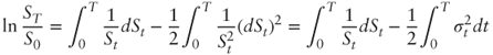
where σt is the underlying asset's instant volatility, which may be stochastic. Rearranging terms, we can see that realized variance may be replicated by continuously maintaining a position of 2/St in the underlying stock and holding onto a certain quantity of log-contracts:
Assuming that the risk-neutral dynamics of the underlying price are of the form ![]() where νt is the risk-neutral drift, we have
where νt is the risk-neutral drift, we have  and thus the fair value of variance matches the fair value of two log-contracts:

The log-contract does not trade, but from Section 3.2 we know that any European payoff can be decomposed as a portfolio of calls and puts struck along a continuum of strikes. Specifically we have the identity:
In other words the log-contract may be replicated with a portfolio which is:
- Short a forward contract on S struck at the forward price F
- Long all puts struck at K < F in quantities dK / K2
- Long all calls struck at K > F in quantities dK / K2
The corresponding fair value of annualized variance is then:
where r is the interest rate for maturity T, p(K) is the price of a put struck at K, and c(K) is the price of a call struck at K.
In practice only a finite number of strikes are available, and we have the proxy formula:

where K1 < ![]() < Kn ≤ F ≤ Kn+1 <
< Kn ≤ F ≤ Kn+1 < ![]() < Kn+m are the successive strikes of n puts worth p(Ki) and m calls worth c(Ki), and ΔKi = Ki – Ki–1 is the strike step.
< Kn+m are the successive strikes of n puts worth p(Ki) and m calls worth c(Ki), and ΔKi = Ki – Ki–1 is the strike step.
A more accurate calculation based on overhedging of the log-contract is discussed in Demeterfi, Derman, Kamal, and Zhou (1999). An alternative derivation of the hedging portfolio and price based on the property that variance swaps have constant dollar gamma can be found in Bossu, Strasser, and Guichard (2005).
5.2.4 Forward Variance
Two variance swaps with maturities T1 < T2 may be combined to capture the forward variance observed between T1 and T2. Indeed under the zero-mean assumption variance is additive and thus:
where ![]() denotes realized volatility between times s and t. Thus:
denotes realized volatility between times s and t. Thus:
This implies that the fair strike of a forward variance swap is:

and, when interest rates are zero, the corresponding hedge is long ![]() variance swaps maturing at T2 and short
variance swaps maturing at T2 and short ![]() variance swaps maturing at T1.
variance swaps maturing at T1.
When interest rates are non-zero, the quantity of the short leg should be adjusted to ![]() because the near-term variance swap payoff at time T1 will carry interest r between T1 and T2.
because the near-term variance swap payoff at time T1 will carry interest r between T1 and T2.
5.3 Realized Volatility Derivatives
Variance swaps are the simplest kind of realized volatility derivatives; that is, derivative contracts whose payoff is a function ![]() of realized volatility. Other examples include:
of realized volatility. Other examples include:
- Volatility swaps, with payoff
- Variance calls, with payoff

- Variance puts, with payoff

Volatility swaps are offered by some banks to investors who prefer them to variance swaps. Deep out-of-the-money variance calls are often embedded in variance swap contracts on single stocks in the form of a cap on realized variance; this is because variance could “explode” when, for instance, the underlying stock is approaching bankruptcy.
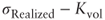
Note that the volatility swap strike Kvol must be less than the variance swap strike Kvar under penalty of arbitrage. This property may also be seen through Jensen's inequality:
The ratio ![]() is called the convexity adjustment by practitioners.
is called the convexity adjustment by practitioners.
Valuing realized volatility derivatives requires a model. Since realized variance is tradable, a natural idea here is to think of it as an underlying asset and apply standard option valuation theory.
However an adjustment is necessary to account for the fact that, as a tradable asset, realized variance is a mixture of past variance and future variance; specifically:
where vt is the forward price of variance started at time 0 and ending at time T, σ(0,t) is the historical volatility observed over [0, t] and Kvar(t,T) is the fair strike at time t of a new variance swap expiring at time T.
Therefore we cannot assume that the volatility of vt is constant as in the Black-Scholes model. Instead we may assume forward-neutral dynamics of the form:
where ω is a volatility of (future) volatility parameter and 2 is a conversion factor from volatility to variance.1 In this fashion the diffusion coefficient ![]() linearly collapses to zero as we approach maturity, as suggested by Equation (5.4).
linearly collapses to zero as we approach maturity, as suggested by Equation (5.4).
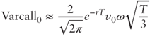
This simple modeling approach allows us to find closed-form formulas for the price of many realized volatility derivatives. For example, the fair strike of a volatility swap can be shown to be:
and thus the convexity adjustment is simply ![]() .
.
Given Kvol and Kvar from the market we may then estimate ω:
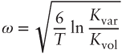
In practice volatility swaps are illiquid but, as suggested by Carr and Lee (2009), the fair value of realized volatility may be approximated with at-the-money implied volatility. For example, if one-year fair variance is 30% and one-year at-the-money implied volatility is 28%, we find ![]() .
.
5.4 Implied Volatility Derivatives
Implied volatility derivatives are derivative contracts whose payoff is a function ![]() of implied volatility. There are many choices for implied volatility and the most popular one is the Volatility Index (VIX) calculated by CBOE, which is the short-term fair variance derived from listed options on the S&P 500 in accordance with Equation (5.3).
of implied volatility. There are many choices for implied volatility and the most popular one is the Volatility Index (VIX) calculated by CBOE, which is the short-term fair variance derived from listed options on the S&P 500 in accordance with Equation (5.3).
The VIX is not a tradable asset, but CBOE nevertheless developed VIX futures and VIX options, which have become increasingly popular.
Specifically, the VIX is a pro rata temporis average of two subindexes based on front- and next-month2 listed options in order to reflect the 30-day expected volatility. Each subindex is calculated according to the generalized formula:

where:
- T is the maturity
- r is the continuous interest rate for maturity T
- F is the forward price of the S&P 500 derived from listed option prices
- K0 is the first strike below F
- Ki is the strike price of the |i|th out-of-the money listed option: a call if i > 0 and a put if i < 0
- ΔKi is the interval between strike prices measured as

- Q(Ki) is the mid-price of the listed call or put struck at Ki.
There are many other practical details that can be found in the CBOE white paper on VIX (2009), such as how exactly the forward price is calculated or how the constituent options are selected.
5.4.1 VIX Futures
VIX futures are futures contracts on the VIX. On the settlement date T the following dollar amount is credited or debited by the exchange:
where 1,000 is the multiplication factor, VIXT is the settlement level3 of the VIX, and Futt is the trading price at time t.
Figure 5.2 shows the term structure of VIX futures as of September 26, 2012. We can see that the curve is upward sloping; however, at times it may be downward sloping because VIX futures, contrary to stock or equity index futures, are not constrained by any carry arbitrage since the VIX is not a tradable asset.
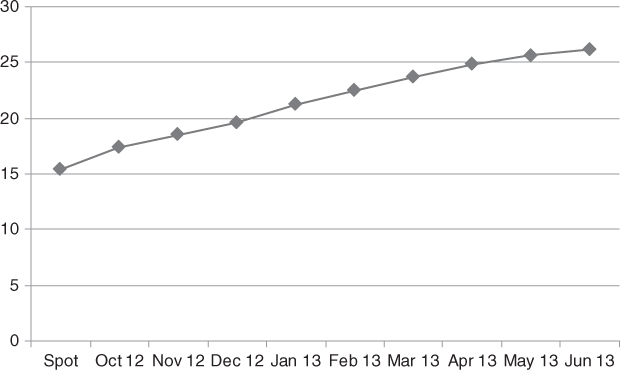
Figure 5.2 Term structure of VIX futures as of September 26, 2012.
Source: Bloomberg.
It is worth emphasizing that VIX futures are bets on the future level of implied volatility, which itself is the market's guess at subsequent realized volatility. In this sense VIX futures are forward contracts on forward realized volatility—a potentially difficult level of “forwardness” to deal with.
Close to expiration, the futures tend to be highly correlated with the VIX. When futures expire in a month, they have about 0.5 correlation with the VIX. Futures that expire in five months or more exhibit almost no correlation.
5.4.2 VIX Options
VIX options are vanilla calls and puts on the VIX. On the settlement date T the following dollar amount is credited or debited by the exchange:
- For a call:

- For a put:
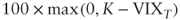
where 100 is the multiplication factor, VIXT is the settlement level4 of the VIX, and K is the strike level.
For lack of a better consensus model, VIX option prices are commonly analyzed through Black's model to compute VIX implied volatilities. Figure 5.3 shows the term structure of at-the-money VIX implied volatility. We can see that the shape is downward sloping: short-term VIX futures are expected to be more volatile than long-term ones.
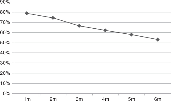
Figure 5.3 Implied volatility term structure of at-the-money VIX options as of September 26, 2012.
Source: Bloomberg.
Similar to VIX futures, VIX option prices tend to have high correlation with the VIX close to expiration and low correlation far away from expiration.
Synthetic put-call parity holds for VIX options, which entails that VIX implied volatility is the same for calls and puts. Specifically:
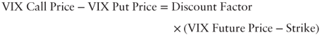
where Discount Factor is the price of $1 paid on the expiration date.
References
- Bossu, Sébastien. 2005. “Arbitrage Pricing of Equity Correlation Swaps.” JPMorgan Equity Derivatives report.
- Bossu, Sébastien, Eva Strasser, and Régis Guichard. 2005. “Just What You Need to Know about Variance Swaps.” JPMorgan Equity Derivatives report.
- Carr, Peter, and Roger Lee. 2009. “Volatility Derivatives.” Annual Review of Financial Economics 1: 1–21.
- Carr, Peter, and Dilip Madan. 1998. “Towards a Theory of Volatility Trading.” In Volatility: New Estimation Techniques for Pricing Derivatives, edited by R. Jarrow, 417–427. London: Risk Books.
- “The CBOE Volatility Index—VIX.” 2009. CBOE White Paper.
- Demeterfi, Kresimir, Emanuel Derman, Michael Kamal, and Joseph Zhou. 1999. “More than You Ever Wanted to Know about Volatility Swaps.” Goldman Sachs Quantitative Strategies Research Notes, March.
Problems
5.1 Delta-Hedging P&L Simulation
Consider a long position in 10,000 one-year at-the-money calls on ABC Inc.'s stock currently trading at $100. Assume zero interest rates and dividends and 30% implied volatility.
- Suppose the “real” stock price process is a geometric Brownian motion with 5% drift and 29% realized volatility. Simulate the evolution of the cumulative delta-hedging P&L with 252 time steps using Equation (5.1). Show one path where the final P&L is positive and one path where it is negative.
- Using 10,000 simulations, compute the empirical distribution of the final cumulative delta-hedging P&L. What is the average P&L?
5.2 Volatility Trading with Options
- You are long a call, which you delta-hedge continuously until maturity. Your cumulative P&L is given by Equation (5.2).
- Suppose the “real” stock price process is a geometric Brownian motion with drift μ and realized volatility σ > σ*. Show that you are guaranteed a positive profit.
- Suppose the “real” stock price process is
 where μt and σt are stochastic with
  . Show that your expected P&L (unconditionally from time 0) is positive.
- b. You are long two one-year calls in quantities q1 and q2 on two independent underlying stocks, which you delta-hedge continuously until maturity. Suppose that the distributions of the two cumulative P&L equations are normal with means m1, m2, and standard deviations s1, s2. What is the distribution of the aggregate cumulative P&L of your option book? Show that its standard deviation must be less than
 .
.
5.3 Fair Variance Swap Strike
Using your SVI calibration results from Problem 2.5 and assuming zero interest rates, estimate the corresponding fair variance swap strike in accordance with Equation (5.3).
5.4 Generalized Variance Swaps
A generalized variance swap has payoff:

where f(S) is a general function of the underlying spot price S, St is the spot price at time t, N is the number of trading days until maturity, and Kgvar is the strike level. Assume zero interest and dividend rates, and that ![]() under the risk-neutral measure.
under the risk-neutral measure.
- Let
 . Using the Ito-Doeblin theorem, show that:
- What can you infer about the fair value and hedging strategy of generalized variance?
- Show that the fair strike is

- Application: corridor variance swap. What does the formula for the fair strike become in case of the corridor variance swap where daily realized variance only accrues at time t when L < St < U?
5.5 Call on Realized Variance
Consider the model ![]() for the forward price at time t of realized variance observed over a fixed period [0,T]. In particular, vT is the terminal historical variance, and v0 =
for the forward price at time t of realized variance observed over a fixed period [0,T]. In particular, vT is the terminal historical variance, and v0 = ![]() (vT) is the undiscounted fair strike of a variance swap at time 0.
(vT) is the undiscounted fair strike of a variance swap at time 0.
- Show that the price of an at-the-money forward call on realized variance with payoff
 is given as:

- Using a first-order Taylor expansion show that