
Chapter 6
Introducing Correlation
Correlation is almost as ubiquitous as volatility in quantitative finance. For example the downward-sloping volatility smile observed in equities may be explained by the negative correlation between stock prices and volatility. In this chapter we introduce various measures of correlation between assets, investigate their properties, and present simple multiasset extensions of the Black-Scholes and Local Volatility models.
6.1 Measuring Correlation
Correlation is the degree to which two quantities are linearly associated. A correlation of +1 or −1 means that the linear relationship is perfect, while a correlation of 0 typically1 indicates independence.
There are two kinds of correlation between two financial assets:
- Historical correlation, based on historical returns;
- Implied correlation, derived from option prices.
6.1.1 Historical Correlation
Historical correlation between two assets S(1) and S(2) is usually measured as the Pearson's correlation coefficient between their N historical returns observed at regular intervals:

where Cov†1,2 is historical covariance, σ†'s are historical standard deviations, ![]() is the return on asset S(j) for observation i, and
is the return on asset S(j) for observation i, and ![]() is the mean return on asset S(j). Returns may be computed on an arithmetic or logarithmic basis; occasionally the mean returns are assumed to be zero.
is the mean return on asset S(j). Returns may be computed on an arithmetic or logarithmic basis; occasionally the mean returns are assumed to be zero.
Figure 6.1 shows the evolution of the historical correlation between Microsoft and Apple over a three-month rolling window since 2000. We can see that this correlation has varied quite significantly over time.

Figure 6.1 Historical correlation of daily returns between Apple and Microsoft over a three-month rolling window since 2000.
Note that using daily returns can produce misleading results for assets trading within different time zones; in this case it is preferable to estimate correlation using weekly returns. Figure 6.2 compares the two methods for the S&P 500 and Nikkei 225 indexes. We can see that the correlation observed on weekly returns is significantly higher.

Figure 6.2 Historical correlation of daily and weekly returns between S&P 500 and Nikkei 225 over a three-month rolling window since 2000.
6.1.2 Implied Correlation
Implied correlation between two assets S(1) and S(2) is derived from an option price, such as a quote for an over-the-counter (OTC) basket option. Typically the quote is converted into an implied basket volatility ![]() from which implied correlation may be extracted through the formula:
from which implied correlation may be extracted through the formula:
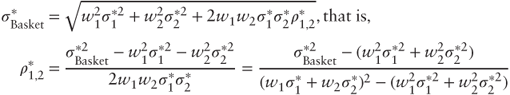
where wj is the weight on asset S(j) and ![]() is the implied volatility of asset S(j).
is the implied volatility of asset S(j).
Conventionally all implied volatilities are for the same moneyness level k (strike over spot) and maturity T, and weights are equal.
6.2 Correlation Matrices
Very often we are interested in correlation for a selection of n ≥ 2 assets. This leads to a correlation matrix of the form:
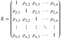
where ρi,j is the pairwise correlation coefficient between assets S(i) and S(j), which may either be historical or implied. Note that R is symmetric because ρi,j = ρj,i.
Not every symmetric matrix with entries in [−1, 1] and a diagonal of 1's is a candidate for a correlation matrix R. This is because the correlation between assets S(i) and S(j) and assets S(j) and S(k) says something about the correlation between assets S(i) and S(k)—intuitively, if Microsoft and Apple are highly correlated, and Apple and IBM are also highly correlated, then Microsoft and IBM must also have some positive correlation.
Figure 6.3 shows the envelope of admissible correlation values when n = 3. We can see that certain regions, such as around the corner (−1, −1, −1) are not admissible.
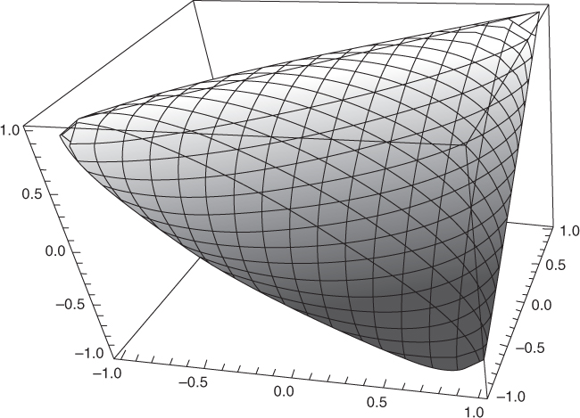
Figure 6.3 Envelope of admissible correlation values when n = 3.
Specifically, correlation matrices must be positive-semidefinite; that is, their eigenvalues must all be nonnegative. This property is always verified for historical correlation but not necessarily for implied correlation. Additionally the sum of all eigenvalues must equal the trace, that is, n.
A common fix for an indefinite candidate matrix M is to replace its negative eigenvalues with zeros and adjust its positive eigenvalues to maintain a sum of n:
where Ω is the orthogonal matrix of eigenvectors of M with eigenvalues (λ1,…, λn) and Dadj is the diagonal matrix of adjusted eigenvalues with entries ![]() . Alternatively one may use the method proposed by Higham (2002).
. Alternatively one may use the method proposed by Higham (2002).
In equities correlation matrices have other empirical properties. Plerou et al. (2002) and Potters, Bouchaud, and Laloux (2005) found for U.S. stocks that the top eigenvalue typically dominates all the other ones. Furthermore, the corresponding eigenvector is more or less an equally weighted portfolio of all the stocks. This suggests that one factor (“the market”) strongly drives the behavior of each stock.
6.3 Correlation Average
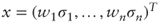
To summarize the overall level of correlation across n assets, it is common practice to compute the average of the correlation matrix, excluding the diagonal of 1's. The formula for a given weighting vector x is then:

where e is the vector of 1's. In the main case of interest where all the weights are nonnegative we have:
but in general ρ(x) could lie outside of these bounds. In practice, when applying sensible weights to a large equity correlation matrix, ρ(x) can safely be assumed to be positive.
Common choices for x are:
- Equal weights: x = e. In this case the average correlation formula simplifies to:
and we have the bounds:
- Market capitalization weights: x = w. This is particularly relevant when the n stocks are the constituents of an equity index such as the S&P 500.
- Volatility and market capitalization weights:
 , where σ's may either be historical or implied volatilities. This case is particularly appealing because of the identity2 or shortcut formula:

where σBasket is the volatility of the all-stock portfolio with weights w. Assimilating an equity index to a portfolio of stocks with fixed weights,3 this formula allows us to compute the average implied correlation using only listed option prices.
In practice, for large baskets (n > 30), these various choices for x tend to produce similar results within a few correlation points, as observed by Tierens and Anadu (2004) and illustrated in Figure 6.4.

Figure 6.4 Realized average correlation for the EuroStoxx 50 index over a six-month rolling window using market capitalization weights and volatility and market capitalization weights.
6.3.1 Correlation Proxy
Equation (6.1) is related to a mathematical quantity known as the Rayleigh quotient ![]() ; specifically, dividing both numerator and denominator by
; specifically, dividing both numerator and denominator by ![]() :
:

where θ is the angle between vectors x and e.
As n → ∞ we have the proxy formula:

subject to certain technical conditions, which are met in practice. In particular, for volatility and market capitalization weights, the proxy formula equates the now well-known squared ratio of basket volatility to average stock volatility:

6.3.2 Some Properties of the Correlation Proxy
We now focus on some fundamental properties of the proxy formula ![]() . In what follows it is assumed that the eigenvalues of R are sorted by ascending order.
. In what follows it is assumed that the eigenvalues of R are sorted by ascending order.
First, a property of the Rayleigh quotient is that it must be comprised between the top and bottom eigenvalues, which implies that:
Note that the lower bound ![]() can be slightly improved in the unconstrained case (see Problem 1) and that tighter numerical bounds can be computed through quadratic optimization methods in the constrained case where x ≥ 0.
can be slightly improved in the unconstrained case (see Problem 1) and that tighter numerical bounds can be computed through quadratic optimization methods in the constrained case where x ≥ 0.
Second, another quantity of interest is the distance between two average correlation measures ![]() . Restricting ourselves to vectors x and y such that
. Restricting ourselves to vectors x and y such that ![]() we may rewrite without loss of generality:
we may rewrite without loss of generality:
The Cauchy-Schwarz inequality then gives the general upper bound ![]() but in practice it is not satisfactory. To find a better upper bound we must look at the spectral decomposition of R:
but in practice it is not satisfactory. To find a better upper bound we must look at the spectral decomposition of R:

where vi is an eigenvector with associated eigenvalue λi. Thus, for any vectors a and b:
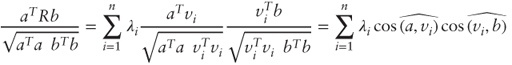
where ![]() denotes the absolute angle in [0, π] between any two vectors u and v.
denotes the absolute angle in [0, π] between any two vectors u and v.
Recalling that the top eigenvalue of stock correlation matrices dominates all other eigenvalues, we are induced to split the sum accordingly:

Furthermore ![]() , so that:
, so that:

We now invoke the fifth property of the Euclidean metric4 to get ![]() ,
, ![]() and for
and for ![]() :
: ![]() , so that:
, so that:

because the eigenvalues sum to n.
Taking ![]() and rearranging terms we get:
and rearranging terms we get:
In practice the quantity between brackets is usually small because x, y are “close” to vn and x + y, x − y are nearly orthogonal.
6.4 Black-Scholes with Constant Correlation
Extending Black-Scholes to a basket of n underlying assets S(1),…, S(n) with constant correlation is fairly straightforward, except perhaps notation-wise.
Given a vector of volatilities (σ1,…, σn) and a correlation matrix (ρi,j), assume that the prices of the underlying assets follow n correlated geometric Brownian motions:

where ![]() . If the derivative's value only depends on time and the n spot prices, we have
. If the derivative's value only depends on time and the n spot prices, we have ![]() and we can apply the multidimensional version of the Ito-Doeblin theorem to get:
and we can apply the multidimensional version of the Ito-Doeblin theorem to get:

where ∇f and ∇2f are the gradient and Hessian of f, respectively.
A portfolio long one unit of derivative and short ![]() units of each asset S(i) is then riskless, and by the same reasoning as in the single-asset case we obtain a multidimensional partial differential equation for f whose only parameters are the interest rate r, the volatility vector and the correlation matrix:
units of each asset S(i) is then riskless, and by the same reasoning as in the single-asset case we obtain a multidimensional partial differential equation for f whose only parameters are the interest rate r, the volatility vector and the correlation matrix:

Solving partial differential equations in high dimension is very hard mathematically and computationally. In practice, the numerical method of choice to implement the multiasset Black-Scholes model is Monte Carlo simulation under the risk-neutral measure. The Cholesky decomposition of the correlation matrix is then typically used to generate correlated Brownian motions from uncorrelated ones.
6.5 Local Volatility with Constant Correlation
Another straightforward extension of a popular model is local volatility with constant correlation (LVCC). Keeping the notations of Section 6.4, this model assumes dynamics of the form:
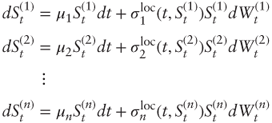
where ![]() is the local volatility function for asset S(i) (see Chapter 4) and
is the local volatility function for asset S(i) (see Chapter 4) and ![]() as before.
as before.
The same reasoning as in Section 6.4 then applies, with identical results after substituting local volatilities. Again Monte Carlo simulations are overwhelmingly preferred to other numerical methods such as multidimensional binomial trees or finite difference lattices.
Until recently the local volatility model with constant correlation was widely used to price a broad range of multiasset exotic options. In Chapter 8, we introduce the next generation of models where correlation is allowed to vary.
References
- Blumenthal, Leonard M. 1933. “On the four-point property.” Bulletin of the American Mathematical Society, 39: 423–426.
- Bossu, Sébastien, and Philippe Henrotte. 2012. An Introduction to Equity Derivatives: Theory and Practice, 2nd ed. Chichester, UK: John Wiley & Sons.
- Dattorro, Jon. 2008. Convex Optimization & Euclidean Distance Geometry. Palo Alto, CA: Meboo Publishing USA.
- De Finetti, Bruno. 1937. “A proposito di correlazione.” Supplemento Statistico ai Nuovi problemi di Politica, Storia ed Economia, 3: 41–57. English translation in Laurence et al. (2008).
- Higham, Nicholas J. 2002. “Computing the Nearest Correlation Matrix—A Problem from Finance.” IMA Journal of Numerical Analysis 22: 329–343.
- Laurence, Peter, Tai-Ho Hwang, and Luca Barone. 2008. “Geometric Properties of Multivariate Correlation in de Finetti's Approach to Insurance Theory.” Electronic Journal for History of Probability and Statistics 4(2).
- Plerou, Vasiliki, Parameswaran Gopikrishnan, Bernd Rosenow, Luis A. Nunes Amaral, Thomas Guhr, and H. Eugene Stanley. 2002. “Random Matrix Approach to Cross Correlations in Financial Data.” Physical Review E 65: 1–18.
- Potters, Marc, Jean-Philippe Bouchaud, and Laurent Laloux. 2005. “Financial Applications of Random Matrix Theory: Old Laces and New Pieces.” Acta Physica Polonica B (36): 2767–2784.
- Tierens, Ingrid, and Margaret Anadu. 2004. “Does It Matter Which Methodology You Use to Measure Average Correlation across Stocks?” Goldman Sachs Equity Derivatives Strategy report, April 2004.
Problems
6.1 Lower Bound for Average Correlation
Let R be a n × n correlation matrix. For any n × n positive-definite matrix A define ![]() where e is the vector of 1's and x is an arbitrary vector which is nonorthogonal to e.
where e is the vector of 1's and x is an arbitrary vector which is nonorthogonal to e.
- Show that
 where λn is the top eigenvalue of R.
 - Show that
 . Hint: This can be formulated as a constrained optimization problem and solved with; for example, the Lagrangian method.
 - We want to approximate the distance
 when R is an equity correlation matrix with top eigenvalue λn
  λn–1 and the corresponding top eigenvector vn is an all-stock portfolio close to e/n (up to a scaling factor).
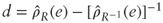
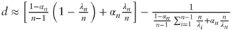
- Show that d may be rewritten as
 where A, H are respectively the arithmetic and harmonic weighted averages of the eigenvalues of R, with weights
 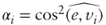 . Hint: Use Parseval's identity to show that
  .
. - Argue that
- Show that d may be rewritten as
6.2 Geometric Basket Call
Consider a call option with payoff ![]() on a geometric basket calculated as
on a geometric basket calculated as ![]() where
where ![]() is the price of the underlying asset S(i) at time t and the nonnegative basket weights (wi) sum to 1.
is the price of the underlying asset S(i) at time t and the nonnegative basket weights (wi) sum to 1.
- a. In the Black-Scholes model with constant correlation, show that under the risk-neutral measure bT is lognormally distributed and find the distribution parameters as functions of volatilities and correlations.
- Find a closed-form formula for the price of the call.
6.3 Worst-Of Put Pricing
Using the Black-Scholes model with constant correlation and Monte Carlo simulations, calculate the price of a one-year at-the-money worst-of put option (see Section 1.2.3) on Apple, Microsoft, and Google, in accordance with the following parameters:
- Interest rate: 1%
- Dividend rates: Apple 3%, Microsoft 2.8%, Google 0%
- Volatilities: Apple 30%, Microsoft 26%, Google 23%
- Correlations: Apple-Google: 35%, Apple-Microsoft: 30%, Google-Microsoft: 50%
6.4 Continuously Monitored Correlation
Consider the LVCC model for two assets S(1) and S(2). Define the continuously monitored realized correlation coefficient as:

Show that ![]()